Enhancing Computational Accuracy in Surrogate Modeling for Elastic–Plastic Problems by Coupling S-FEM and Physics-Informed Deep Learning

Abstract

Physics-informed neural networks (PINNs) provide a new approach to solving partial differential equations (PDEs), while the properties of coupled physical laws present potential in surrogate modeling. However, the accuracy of PINNs in solving forward problems needs to be enhanced, and solving inverse problems relies on data samples. The smoothed finite element method (S-FEM) can obtain high-fidelity numerical solutions, which are easy to solve for the forward problems of PDEs, but difficult to solve for the inverse problems. To the best of the authors’ knowledge, there has been no prior research on coupling S-FEM and PINN. In this paper, a novel approach that couples S-FEM and PINN is proposed. The proposed approach utilizes S-FEM to synthesize high-fidelity datasets required for PINN inversion, while also improving the accuracy of data-independent PINN in solving forward problems. The proposed approach is applied to solve linear elastic and elastoplastic forward and inverse problems. The computational results demonstrate that the coupling of the S-FEM and PINN exhibits high precision and convergence when solving inverse problems, achieving a maximum relative error of 0.2% in linear elasticity and 5.69% in elastoplastic inversion by using approximately 10,000 data points. The coupling approach also enhances the accuracy of solving forward problems, reducing relative errors by approximately 2–10 times. The proposed coupling of the S-FEM and PINN offers a novel surrogate modeling approach that incorporates knowledge and data-driven techniques, enabling it to solve both forward and inverse problems associated with PDEs with high levels of accuracy and convergence.

1. Introduction

Partial differential equations (PDEs) are essential in engineering applications, as most natural and complex systems are governed by physical phenomena that can be described by PDEs [1,2,3]. However, finding solutions to most PDEs poses a significant challenge and often requires complex numerical techniques. Currently, the finite element method (FEM) [1,4], the finite difference method (FDM) [5], and the material point method (MPM) [6] are the primary numerical methods used for solving PDEs. Discretization is often necessary when solving complex PDEs by using numerical methods, such as FEM, FDM, and MPM. The computational efficiency and accuracy of a model are closely linked to the mesh density and computational step size.

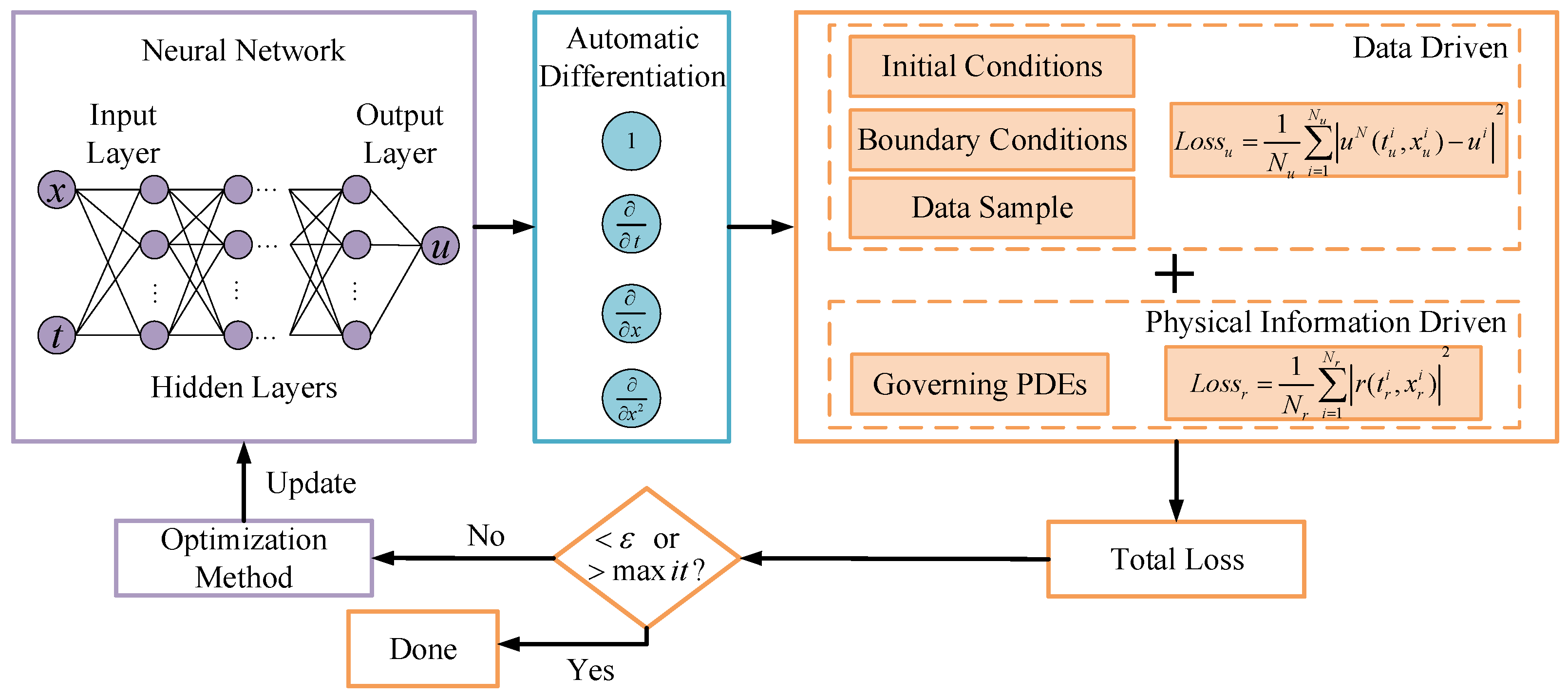
Physics-informed deep learning, which has emerged in recent years, is based on novel ideas for solving PDE problems [7]. An example of this is physics-informed neural networks (PINNs), which are typical representatives that utilize automatic differentiation to incorporate PDEs into the loss function of the neural network. This approach can solve various types of PDEs accurately, and the computational accuracy remains unaffected by variations in computational step size [8,9,10]. As a result, compared to traditional numerical methods, the solving process and results for high-dimensional PDE problems are no longer restricted. In addition, the PINN framework can tackle the inverse problems associated with PDEs by inferring the unknown coefficient and/or source terms of the governing equations from measured data [8]. PINNs are a class of neural networks designed for solving supervised learning tasks that are required to satisfy not only the constraints of the training samples but also the physical information constraints of the PDEs [7,11]. Compared to purely data-driven neural networks, PINNs incorporate physical information constraints into the training process. Hence, the utilization of fewer data samples to learn more generalized models is possible [7,12]. In recent years, PINN has become an increasingly popular research topic at the intersection of machine learning and computational mathematics and has made significant progress in both theory and applications [7,8,13,14,15,16,17,18,19,20,21,22].

For example, Raissi et al. [8] employed PINN to accurately solve the Schrödinger and Allen–Cahn equations, as well as to perform parameter inversions of the Navier–Stokes and Korteweg–de Vries equations. Ehsan Haghighat et al. [13] developed SciANN, an artificial neural network framework based on Python, to solve both the forward and inverse problems of PDEs using the PINN approach. Lu et al. [14] introduced the residual-based adaptive refinement (RAR) method and the construction geometry method to enhance the training efficacy of the PINN in complex computational domains. They also created a Python toolkit called DeepXDE, based on TensorFlow. DeepXDE has the capability to solve both forward problems, based on initial and boundary conditions, and inverse problems, taking into account additional measurements [14]. Jagtap et al. [15] proposed a scalable hyperparameter for the activation function of the PINN to enhance its efficiency. This hyperparameter optimizes the network’s performance by dynamically adjusting the loss function involved in the optimization process.

Researchers are increasingly focusing on combining traditional numerical methods with deep learning techniques to solve PDEs. For instance, Milan et al. [23] proposed a hybrid approach that combines finite-volume-based CFD simulations with neural networks to accelerate the simulation of high-pressure fluid flow in propulsion applications while reducing the memory footprint. Kochkov et al. [24] recently proposed an end-to-end deep learning approach to improve computational fluid dynamics for turbulence and large eddy simulations. The proposed method offers a remarkable acceleration factor of 40 to 80 while maintaining some stability over long simulations [24]. Zhang et al. [25] introduced HiDeNN-FEM, a hierarchical deep neural network representing the FEM, which has demonstrated its potential in solving multidimensional higher-order continuity and topology optimization problems. Moreover, Mitusch et al. [26] proposed a hybrid FEM-NN model that shows good convergence for multiple types of PDEs. Moreover, Uriarte et al. [27] proposed a deep learning approach for solving linear parametric PDEs using FEM, which utilizes a neural network architecture to simulate the finite element refinement mesh, thereby improving the interpretability and accuracy of numerical integration in deep learning.

Although many researchers have successfully combined traditional numerical methods with deep learning to solve difficult problems, the implementation of these approaches is complicated, and it is challenging to solve both forward and inverse problems simultaneously. PINN offers a novel approach to solving PDEs, and its ability to handle coupled physical laws demonstrates its potential as a surrogate model [8]. PINN can serve as an integrated method for both training and identification purposes. During PDE solving, unknown parameters in the equation can be identified directly based on additional information. When solving forward problems, PINN only requires information about the control equations, initial conditions, and boundary conditions, and does not rely on any data. However, its computational accuracy is lower than traditional numerical computation methods [12]. Moreover, PINN can solve inverse problems using partial data samples, which may include real field data, exact solutions to the problem, or high-fidelity synthetic data [28]. In practical engineering problems, exact solutions are seldom attainable, and acquiring enough real field data can be arduous. Therefore, numerical calculation methods are generally utilized to synthesize the dataset required for training.

The smoothed finite element method (S-FEM), which combines the FEM with the strain smoothing technique, is a new numerical method introduced by Liu G. R. et al. [29] in recent years. By employing strain smoothing techniques, the S-FEM eliminates the need for coordinate mapping and Jacobian transformations, which helps to prevent computational errors and inaccuracies caused by mesh distortions in complex models [29]. Moreover, the low-order S-FEM can achieve the same level of computational accuracy as the high-order FEM while simultaneously reducing computational complexity and costs for obtaining high-fidelity numerical solutions. S-FEM represents a numerical technique that integrates the benefits of FEM and meshless methods. In the context of inverse problems, these methods demonstrate similarities to FEM and are frequently augmented with optimization algorithms [30,31,32]. The present research is mainly directed toward solving inverse problems related to geometric heat conduction through the integration of the smooth gradient concept of the S-FEM with the fixed grid FEM [33,34].

To enhance the computational accuracy of the PINN and overcome the limitation of the S-FEM for solving inverse problems [33,34], we propose a novel method that couples S-FEM with the PINN to solve the forward and inverse problems of PDEs. The S-FEM is employed to create a high-precision dataset that is necessary for the PINN inversion process. Initially, the material parameter combinations to be inverted are determined, followed by selecting multiple sets of material parameter combinations as inputs for the smoothed finite element simulation, within the limits of reasonable values of these parameters. The displacement–stress data are then calculated using the S-FEM. The displacement and stress data are subsequently incorporated into the loss function component of the PINN as data constraints that operate in conjunction with physical constraints to invert the unknown material parameters. The primary benefit of the pure PINN in resolving forward problems of PDE is its freedom from data dependence, which permits its solution via the control equations, and initial and boundary conditions. However, its precision is comparatively lower than that of more established numerical computational techniques [12]. Consequently, a high-precision dataset created through S-FEM is incorporated into the loss function component of the PINN that solves PDEs without data dependence. The integration of data-driven and physics-informed coordination improves the accuracy of the PINN without data dependence. To verify the computational accuracy of the S-FEM-coupled PINN, we solve the linear elastic and elastoplastic forward and inverse problems using this coupling method. The results of this solution will be used to compare the accuracy with that of pure S-FEM and PINN for solving the same problem.

The rest of this paper is organized as follows. Section 2 provides an overview of physics-informed deep learning and the S-FEM. Section 3 introduces the three equations of linear elastic problems, the constitutive relations of elastoplastic problems, and the implementation of the S-FEM-coupled PINN. Section 4 analyzes the accuracy of the S-FEM-coupled PINN in comparison with S-FEM and PINN in solving linear elastic and elastoplastic problems through examples. Section 5 presents a discussion on the benefits and limitations of coupling S-FEM with the PINN, along with the potential directions for future research. Finally, Section 6 summarizes the contents of this paper.

2. Background

In this section, we provide a brief introduction to the physics-informed deep learning and smoothed finite element method.

2.1. Physics-Informed Deep Learning

The most widely utilized physics-informed deep learning algorithmic framework is the PINN proposed by Professor Karniadakis and his collaborators [7,8]. PINN is mainly used for solving forward and inverse problems for PDEs [8]. In the PINN framework, a fully connected feed-forward neural network is used as the core of surrogate modeling to predict the output of the PDEs. The automatic differentiation of the neural network is also used to control the differential operator in the PDEs [35]. The main idea of the neural network approach to solving PDEs is to use neural networks and sample data possessing partial differential properties to approximate the explicit form of the PDEs in the corresponding region. The process of modeling PDEs involves searching for nonlinear functions that meet specific constraints. In contrast, neural networks are considered versatile approximators of nonlinear functions, thus sharing similarities with the former [7]. Due to the prevalent use of automatic differentiation techniques in deep neural networks, we can effectively integrate the differential form constraints derived from PDEs into the design of the neural network’s loss function [8]. In this way, neural networks that adhere to physical constraints are obtained. This is the essential idea behind PINNs. The neural network trained in this manner not only approximates the observed data but also inherently satisfies the physical properties, such as symmetry, invariance, and conservation of the PDEs, due to the incorporation of physical constraints in the loss function during training [8]. The subsequent section illustrates the design methodology of the PINN using a generic form of PDEs as an example. Specifically, let the function $u=u(t,x)$ satisfy a PDE of the following form.

$$u_t+N(u,\lambda )=0,x\in \mathsf{\Omega },t\in [0,T]$$

(1)

where $N(u,\lambda )$ is a generic function with parameter $\lambda$ that differentiates with respect to u, x is a space variable, t is a time variable, $\mathsf{\Omega }$ is a subset of the Euclidean space $R^D$, and T is the termination moment. Given the initial state of $u(t,x)$, boundary conditions, and physical parameters $\lambda$, the traditional physical model can solve the PDEs to predict the value of $u(t,x)$ at any point in time and space. When an analytical solution is not available, numerical methods such as the FEM and the FDM can be used to solve the equation. While the PINN establishes a neural network as an alternative model to approximate the solution of the PDEs, we define $u^N(t,x)$ as the neural network that approximates the function $u(t,x)$, $r(t,x)=u_t^N+N(u^N,\lambda )$ as the residual of the PDEs, and we define the loss function of the PINN, $Loss=Los{s}_u+Los{s}_r$, where

$$Los{s}_u=\frac{1}{N_u}\sum _{i=1}^{N_u}{\left|u^N(t_u^i,x_u^i)-u^i\right|}^2$$

(2)

$$Los{s}_r=\frac{1}{N_r}\sum _{i=1}^{N_r}{\left|r(t_r^i,x_r^i)\right|}^2$$

(3)

Equation (2) represents the data-driven part of the loss function, i.e., the training data obtained through the initial state and boundary conditions in the forward problem (and the training data obtained through experimental observations, numerical simulations, etc. in the inverse problem). Equation (3) represents the physics-informed part of the loss function, which is the residual value of the training points of the PDEs obtained using automatic differentiation techniques.

To be able to train a neural network that approximates a function $u^N(t,x)$ that satisfies the constraints of the PDEs in addition to minimizing the error with the label data, the PINN solution principle depicted in Figure 1 is adopted. After inputting time and space data, the function is first approximated by a neural network. Subsequently, automatic differentiation techniques are utilized to derive the residuals of the PDEs and the constraints of the initial value residual, which are then incorporated into the loss function as regularization terms. Finally, an optimization algorithm, such as gradient descent, is employed to minimize the loss function, allowing for the determination of the neural network connection weight parameters and the physical parameters of the PDEs.

2.2. Smoothed Finite Element Method

In recent years, several effective numerical methods have been proposed to enhance the performance of low-order FEM in problem-solving, particularly in improving computational accuracy and preventing volume and shear locking [29,36,37,38]. The S-FEM, which combines the FEM with the strain smoothing technique, was proposed by Liu G.R. and his research team [29]. In S-FEM, the shape function is constructed in the same element form as FEM, and the smoothing operation is performed on a separate smoothing domain than that used in FEM. The workflow of the S-FEM is similar to that of FEM, with the key difference being that all calculations in S-FEM are carried out on the smoothing domain, whereas in FEM, all calculations are performed on the finite element mesh.

Currently, there are four approaches to constructing smoothing domains: (1) A cell in a finite element is regarded as a fundamental unit, and it is further divided into several sub-cell domains to form a cell-based smoothing domain. (2) A cell node in a finite element is taken as a fundamental unit, and the closed area formed by connecting the node and the centroids of its adjacent elements is a node-based smoothing domain. (3) A cell edge in a finite element is regarded as a fundamental unit, and the closed region formed by connecting the nodes of the edge and the centroids of its adjacent elements is an edge-based smoothing domain. (4) A cell face in a finite element is taken as a fundamental unit, and the closed area formed by connecting the nodes of the face and the centroids of its adjacent elements is a face-based smoothing domain. The four smoothing domain construction methods correspond to four S-FEMs, i.e., the cell-based S-FEM (CS-FEM) [39,40], node-based S-FEM (NS-FEM) [41], edge-based S-FEM (ES-FEM) [42,43], and face-based S-FEM (FS-FEM) [44]. In addition to the above four methods, there are also hybrid S-FEM [45,46], improved S-FEM [47,48], etc. The smoothing domains of CS-FEM exist in the interior of the element, while the smoothing domains of other methods exist between adjacent elements. The smoothing domains are linearly independent, ensuring the stability and convergence of the S-FEM model. At the same time, due to the strain smoothing technique used in the smoothing domain calculation, the over-rigidity of the finite element model is further reduced, and the accuracy of the displacement and stress calculation results is greatly improved [29,49].

3. Materials and Methods

In this section, we introduce the three equations of linear elastic problems, the constitutive relations of elastoplastic problems, and the implementation of the S-FEM-coupled PINN.

3.1. Linear Elasticity

To describe linear elastic problems, three primary equations are used: (1) the equilibrium differential equation, which represents the momentum balance relationship; (2) the physical equation, which represents the constitutive relationship; and (3) the strain compatibility equation, which represents the kinematic relationship. These equations are shown below:

$${\sigma }_{ij,j}+f_i=0$$

(4)

$${\sigma }_{ij}=\lambda {\delta }_{ij}{\epsilon }_{kk}+2\mu {\epsilon }_{ij}$$

(5)

$${\epsilon }_{ij}=\frac{1}{2}(u_{i,j}+u_{j,i})$$

(6)

where ${\sigma }_{ij}$ is the stress tensor. For two-dimensional problems, here, $i,j=1,2\left(ori,j=x,y\right)$. The function $f_i$ represents the volume force, $u_i$ is the displacement, ${\epsilon }_i$ is the strain tensor, and ${\delta }_i$ is the Kronecker symbol. The summation convention is used here [50], with subscript commas indicating partial derivatives. The forward problem of linear elastic PDEs is to solve its displacement field, stress field, and strain field, and the inverse problem is to solve the material parameters $\lambda$ and $\mu$.

3.2. Elastoplasticity

The appropriate selection and use of the constitutive relation is crucial in correctly solving elastoplastic problems. In this paper, the von Mises yield criterion is utilized to determine whether the material has entered the plastic stage. The power-hardening stress–strain relationship represents the constitutive relationship of the material, and the total strain theory is adopted to solve elastoplastic problems.

The von Mises yield criterion:

$$\overline{\sigma }=\frac{1}{\sqrt{2}}\sqrt{{\left({\sigma }_{xx}-{\sigma }_{yy}\right)}^2+{\left({\sigma }_{yy}-{\sigma }_{zz}\right)}^2+{\left({\sigma }_{zz}-{\sigma }_{xx}\right)}^2+6\left({\tau }_{xy}^2+{\tau }_{yz}^2+{\tau }_{zx}^2\right)}={\sigma }_s$$

(7)

where $\overline{\sigma }$ is the equivalent stress calculated according to Equation (7), ${\sigma }_s$ is the yield stress of the material, and the material enters the plastic phase when $\overline{\sigma }={\sigma }_s$.

To make the power-hardening stress–strain curve satisfy the Hooke law when $\overline{\epsilon }\le {\epsilon }_s$, the following stress–strain relationship is adopted:

$$\overline{\sigma }=\left\{\begin{array}{c}E\overline{\epsilon }\left(0\le \overline{\epsilon }\le {\epsilon }_s\right)\hfill \\ B{\left(\overline{\epsilon }-{\epsilon }_0\right)}^m\left(\overline{\epsilon }\ge {\epsilon }_s\right)\hfill \end{array}\right.$$

(8)

where E is the Young’s modulus, m is the power-hardening index, and ${\epsilon }_s$ is the equivalent strain corresponding to the yield stress ${\sigma }_s$ of the material. To ensure that $\overline{\sigma }$ and $\frac{d\overline{\sigma }}{d\overline{\epsilon }}$ are continuous at $\overline{\epsilon }={\epsilon }_s$, the values of ${\epsilon }_0$ and B are taken as follows:

$${\epsilon }_0={\epsilon }_s\left(1-m\right)$$

(9)

$$B=\frac{E{\epsilon }_s}{{\left({\epsilon }_s-{\epsilon }_0\right)}^m}$$

(10)

The complete expression of the total strain theory can be found in Equations (11)–(13).

$$e_{ij}=\frac{3}{2}\frac{\overline{\epsilon }}{\overline{\sigma }}{s}_{ij}$$

(11)

$$\overline{\sigma }=\phi \left(\overline{\epsilon }\right)$$

(12)

$${\sigma }_m=3K{\epsilon }_m$$

(13)

In Equation (11), $e_{ij}={\epsilon }_{ij}-{\epsilon }_m{\delta }_{ij}$ is the deflection strain tensor, $s_{ij}={\sigma }_{ij}-{\sigma }_m{\delta }_{ij}$ is the deflection stress tensor, $\overline{\epsilon }=\sqrt{2/3e_{ij}{e}_{ij}}$ is the equivalent strain, and $\overline{\sigma }=\sqrt{3/2s_{ij}{s}_{ij}}$ is the equivalent stress. Equation (12) is calculated in this paper using the power-hardening form of Equation (8). In Equation (13), ${\sigma }_m=\left({\sigma }_{xx}+{\sigma }_{yy}+{\sigma }_{zz}\right)/\phantom{\left({\sigma }_{xx}+{\sigma }_{yy}+{\sigma }_{zz}\right)3}3$ is the mean stress, ${\epsilon }_m=\left({\epsilon }_{xx}+{\epsilon }_{yy}+{\epsilon }_{zz}\right)/\phantom{\left({\epsilon }_x+{\epsilon }_y+{\epsilon }_z\right)3}3$ is the mean strain, and K is the bulk modulus.

3.3. Workflow of the S-Fem

In a solid mechanics problem, the problem domain is denoted by $\mathsf{\Omega }$, and the boundary is denoted by $\mathsf{\Gamma }={\mathsf{\Gamma }}_u\cup {\mathsf{\Gamma }}_t$. The essential boundary is represented by ${\mathsf{\Gamma }}_u$, while the natural boundary is represented by ${\mathsf{\Gamma }}_t$. The workflow of the S-FEM is illustrated in Figure 2 and the detailed procedures and operations are as follows [29,36,49]:

(1) The discretization of the problem domain. The S-FEM can use arbitrary polygonal elements to discretize the problem domain. Generally, triangular or quadrilateral elements are used to discretize two-dimensional domains, while tetrahedral or hexahedral elements are employed for three-dimensional domains.

(2) Construction of shape functions to create displacement fields.

(3) Construction of a strain smoothing field. The strain smoothing technique can be used directly on the smoothing domain to construct a strain smoothing field using the shape function values for any type of cell. This procedure requires only a line or area partition directly on the boundary of the smoothing domain, without coordinate mapping. This characteristic is also the reason why the S-FEM is insensitive to mesh distortions.

(4) Establishment of a discrete linear algebraic system of equations. The assumed displacement field and the strain smoothing field are used to establish a discrete linear algebraic system of equations through the smoothing Galerkin method. In the S-FEM, this process only involves simple summation operations for the relevant parameters of the smoothing domain.

(5) Imposition of boundary conditions and system equation solutions to obtain displacement solutions.

(6) Reconstruction of the strain field using the obtained displacement solution. The stress of the equivalent node is obtained in the smoothing domain using the weighted average method, and the continuous stress field in the problem domain is then obtained using the shape function interpolation method.

3.4. Neural Network Setup

In this paper, a fully connected neural network is implemented within the deep learning framework of TensorFlow using Python language. For the elastoplastic statics problem, the input of the neural network is the node spatial coordinates and the output is the node displacements and stresses. For the elasticity problem, the material parameters for the inversion are the Lamé parameters $\lambda$, $\mu$ in Equation (5). For the elastic–plastic problem, the parameters that need to be inverted are $\lambda$, $\mu$, and ${\sigma }_s$. Moreover, ${\sigma }_s$ corresponds to ${\epsilon }_s$ in Equation (8), which is the condition for determining whether the material enters plasticity in Equation (7). According to the control equations, initial conditions, boundary conditions, and sample point data, constraints are set and loss functions are computed. The physical quantities obtained from the network’s output and those labeled in the training samples are substituted into the PDEs, boundary condition, and initial condition. The difference between the two is then used to construct a loss function. The connection weights between each neuron in the neural network are adjusted by minimizing the loss function to achieve convergence.

The Adam optimizer is selected for gradient descent optimization, and tanh is used as the activation function of the neural network. The parameters of the neural network model are selected and set according to the specific problem, mainly including batch size, learning rate, learning rate decay, epochs/iterations, adaptive weights, initializer, etc. The loss function was calculated using the mean squared error (MSE). After the neural network model is established, the model is compiled first, and then the model is trained. Optimization methods are used to continuously minimize the loss function to make the neural network converge and obtain the parameter values for the inversion. Finally, the unknown displacement and stress fields of the model are predicted. The PINN structure used in this paper for the inverse elastoplastic static problem is illustrated in Figure 3.

3.5. The Implementation of the S-FEM-Coupled PINN

In the elastic–plastic inverse problem, data for pure PINNs are typically obtained from either measured data or synthesized data from numerical methods (such as FEM). However, obtaining measured data can be challenging, while synthesized data from numerical methods may be less accurate or more expensive. In contrast, the coupling method uses synthesized data from the S-FEM, which is easier to obtain than measured data and has higher accuracy and lower cost than FEM.

To solve the inverse problem with S-FEM-coupled PINN, material parameters are set as unknown variables in the PINN, which are identified during the training process. The input of the PINN consists of spatial coordinates, while its output involves displacement and stress fields. In the elastoplastic statics problem, the unidentified material parameters include the Lamé parameter and the yield stress. As presented in Figure 4, the proposed method in this paper starts by discretizing the problem domain using the S-FEM to obtain the spatial coordinates of a series of nodes, which are then used as input variables for PINN. The smoothing domain, displacement field, and smoothed strain field are constructed based on the S-FEM calculation procedure. On this basis, the smoothed stiffness matrix is calculated and assembled. Finally, the system equations are solved after imposing the boundary conditions to obtain the nodal displacements and equivalent nodal stress of the problem. These values are then embedded as data constraints in the loss function of the PINN. The physical constraints, including the equilibrium differential equations, geometric equations, and physical equations of the elastic–plastic problem, are also embedded in the loss function of the PINN. The physical loss and data loss are combined as the total loss function, which is optimized using optimization methods to continuously reduce the value of the loss function. This results in the neural network output being gradually closer to the true value. A threshold value or a maximum number of iteration steps is used to determine whether to continue the training of the neural network or not. The material parameters obtained from the inversion of each iteration step of the training process are output to facilitate the analysis of the inversion results. The algorithmic flowchart for the implementation and training of the S-FEM-coupled PINN in TensorFlow is illustrated in Figure 5.

In the elastoplastic forward problems, pure PINNs solve the forward problem without known data and are optimized by embedding boundary conditions, equilibrium differential equations, geometric equations, and physical equations into the loss function. The coupling method improves the solution accuracy by incorporating synthesized data from the S-FEM and using both physical and data constraints in the loss function. By adding constraints, the coupling method combines the advantages of both methods and achieves more accurate and efficient solutions.

To solve the forward problem with S-FEM-coupled PINN, the material parameters are known and the spatial coordinates serve as the input to the PINN, while the output is the displacement and stress fields. To obtain the spatial coordinates, a small-scale discretization of the problem domain is carried out using the S-FEM. The nodal displacements and equivalent nodal stress values are then obtained using the S-FEM and used as data constraints in the loss function of the PINN. The boundary conditions, equilibrium differential equations, and physical equations of the elastoplastic problem are also embedded in the loss function of the PINN. The neural network is trained to minimize the loss function, thereby achieving convergence. Once trained, the neural network can be used to predict the displacement and stress of a large-scale node with the same geometric boundary conditions.

4. Results and Analysis

In this section, we analyze the results of the forward and inverse problems of the S-FEM-coupled PINN for practical examples of the linear elastic and elastoplastic problems. Furthermore, a comparative analysis is conducted between the forward problem results of the S-FEM and PINN with those obtained from the coupled approach.

4.1. Linear Elasticity

4.1.1. Problem Setup

To evaluate the accuracy of the S-FEM-coupled PINN in solving PDEs, a linear elastic plane strain problem was solved using three different methods: S-FEM-coupled PINN, S-FEM, and PINN. The geometric model and boundary conditions of the problem were adopted from the literature [28], and are illustrated in Figure 6. The linear elastic plane strain problem involves three main types of PDEs:

(1) Equilibrium differential equations. See Equations (14) and (15).

$${\sigma }_{xx,x}+{\sigma }_{xy,y}+f_x=0$$

(14)

$${\sigma }_{xy,x}+{\sigma }_{yy,y}+f_y=0$$

(15)

(2) Geometric equations. See Equations (16)–(18).

$${\epsilon }_{xx}=u_{x,x}$$

(16)

$${\epsilon }_{yy}=u_{y,y}$$

(17)

$${\epsilon }_{xy}=\frac{1}{2}(u_{x,y}+u_{y,x})$$

(18)

(3) The stresses obtained from the equilibrium differential equation and the strains obtained from the geometric equation are substituted into the following physical equations. See Equations (19)–(21).

$$(\lambda +2\mu ){\epsilon }_{xx}+\lambda {\epsilon }_{yy}-{\sigma }_{xx}=0$$

(19)

$$(\lambda +2\mu ){\epsilon }_{yy}+\lambda {\epsilon }_{xx}-{\sigma }_{yy}=0$$

(20)

$$2\mu {\epsilon }_{xy}-{\sigma }_{xy}=0$$

(21)

The model illustrated in Figure 6 is subjected to volume forces in the x-direction and y-direction, denoted by $f_x$ and $f_y$, respectively, as described in Equations (22) and (23).

$$\begin{array}{ccc}\hfill f_x& =& \lambda [4{\pi }^{2}cos\left(2\pi x\right)sin\left(\pi y\right)-\pi cos\left(\pi x\right)Q{y}^3]\hfill \\ \hfill & +& \mu [9{\pi }^{2}cos\left(2\pi x\right)sin\left(\pi y\right)-\pi cos\left(\pi x\right)Q{y}^3]\hfill \end{array}$$

(22)

$$\begin{array}{ccc}\hfill f_y& =& \lambda [-3sin\left(\pi x\right)Q{y}^2+2{\pi }^{2}sin\left(2\pi x\right)cos\left(\pi y\right)]\hfill \\ \hfill & +& \mu [-6sin\left(\pi x\right)Q{y}^2+2{\pi }^{2}sin\left(2\pi x\right)cos\left(\pi y\right)+{\pi }^{2}sin\left(\pi x\right)Q{y}^4/4]\hfill \end{array}$$

(23)

where $\lambda$ and $\mu$ are material parameters that are required to be identified using the S-FEM-coupled PINN, the true values of $\lambda$ and $\mu$ are 1 and 0.5, respectively, and Q is the applied load and has a value of 4.

The exact solution to the displacement of the linear elastic plane strain problem can be computed from Equations (24) and (25).

$$u_x(x,y)=cos\left(2\pi x\right)sin\left(\pi y\right)$$

(24)

$$u_y(x,y)=sin\left(\pi x\right)Q{y}^4/4$$

(25)

Figure 6. Illustration of geometric and boundary conditions for the linear elastic plane strain problem.

Figure 6. Illustration of geometric and boundary conditions for the linear elastic plane strain problem.

According to the above conditions, the data loss part of the PINN corresponding to the linear elasticity problem is shown in Equation (26); and the PDE loss part is shown in Equation (27).

$$\begin{array}{ccc}\hfill Los{s}_u& =& \frac{1}{N}\sum _{i=1}^N\left({\left|u_x^i-u_x^{i*}\right|}^2+{\left|u_y^i-u_y^{i*}\right|}^2+{\left|{\sigma }_{xx}^i-{\sigma }_{xx}^{i*}\right|}^2\right.\hfill \\ \hfill & +& {\left|{\sigma }_{yy}^i-{\sigma }_{yy}^{i*}\right|}^2\left.+{\left|{\sigma }_{xy}^i-{\sigma }_{xy}^{i*}\right|}^2\right)\hfill \end{array}$$

(26)

$$\begin{array}{ccc}\hfill Los{s}_r& =& \frac{1}{N}\sum _{i=1}^N{\left({\left|{\sigma }_{xx,x}^i+{\sigma }_{xy,y}^i+f_x^{i*}\right|}^2+\left|{\sigma }_{xy,x}^i+{\sigma }_{yy,y}^i+f_y^{i*}\right|\right.}^2\hfill \\ \hfill & +& {\left|(\lambda +2\mu ){\epsilon }_{xx}^i+\lambda {\epsilon }_{yy}^i-{\sigma }_{xx}^i\right|}^2+{\left|(\lambda +2\mu ){\epsilon }_{yy}^i+\lambda {\epsilon }_{xx}^i-{\sigma }_{yy}^i\right|}^2\hfill \\ \hfill & +& \left.{\left|2\mu {\epsilon }_{xy}^i-{\sigma }_{xy}^i\right|}^2\right)\hfill \end{array}$$

(27)

where the physical quantity marked with an asterisk is the known data and N is the number of sample points of the input data.

4.1.2. The Results of the S-FEM-coupled PINN

For the linear elastic plane strain problem illustrated in Figure 6, we adopt the S-FEM-coupled PINN to perform material parameter inversion for the Lamé parameters, $\lambda$ and $\mu$. Firstly, we utilize the S-FEM to generate 16 × 16 quadrilateral element node data based on the computational process outlined in Section 3.3. Next, we imported the displacement and stress data obtained into the PINN, which was constructed in Section 3.4. The neural network parameters are set according to

Table 1. The neural network parameters for solving the linear elastic inverse problems.

Neural Network Parameters	Values
Layers	[40] × 4
Activation Functions	tanh
Batch Size	64
Learning Rate	0.001
Epochs	4000
Initializer	Glorot uniform

, with the data loss component and the physical loss component given equal importance, and their weights are set as 1. The material parameters $\lambda$ and $\mu$ are initialized as unknown variables, with an initial value of 2.0. We initialize the neural network by the Glorot uniform method, which initializes the input tensor by drawing samples from a uniform distribution within $\left. [-\mathrm{limit},\mathrm{limit}\right]$, where $\mathrm{limit}=\sqrt{(6/(fan\_in+fan\_out\left)\right)}$ ($fan\_in$ is the number of input units in the weight tensor and $fan\_out$ is the number of output units). Following the above methods for parameter and network initialization, we optimize the training process, and invert $\lambda$ and $\mu$.

The variation in the identification of material parameters with an increasing number of training steps is illustrated in Figure 7. It can be seen that the inversion results for both material parameters reach convergence at approximately 3000 training steps. The relative error between the convergence of the inversion result of parameter $\lambda$ at 0.935 and its true value of 1.0 is 6.5%, and the relative error between the convergence of the inversion result of parameter $\mu$ at 0.487 and its true value of 0.5 is 2.6%.

Given the small-scale dataset used in the implementation of the linear elasticity problem, the parameter inversion results are not as accurate. To address this, a comparative analysis of the inversion results of different scale datasets was conducted. Four datasets of sizes 16 × 16, 32 × 32, 64 × 64, and 128 × 128 were synthesized using S-FEM and coupled with the PINN for inversion. The convergence of the inversion results was observed in Figure 8, where the results reached convergence at approximately 3000 training steps for the 16 × 16 dataset and approximately 100 steps for the 128 × 128 dataset. The convergence of the parameter inversion results is significantly faster with an increase in the size of the dataset. The relative error between the inversion results and the actual values was compared in

Table 2. Comparison of the relative errors between the inversion results and the true values of the linear elasticity parameter $\lambda$ for different data sizes.

Data	Exact	Predicted	Relative Error
16 × 16	1.000	0.935	6.5%
32 × 32	1.000	0.963	3.7%
64 × 64	1.000	0.990	1.0%
128 × 128	1.000	0.998	0.2%

and

Table 3. Comparison of the relative errors between the inversion results and the true values of the linear elasticity parameter $\mu$ for different data sizes.

Data	Exact	Predicted	Relative Error
16 × 16	0.500	0.487	2.6%
32 × 32	0.500	0.499	0.2%
64 × 64	0.500	0.500	0
128 × 128	0.500	0.500	0

, where it is observed that the parameter $\mu$ could be accurately identified with an error of 0 when the dataset increased to 64 × 64. Additionally, the relative error of the parameter $\lambda$ was only 0.2% when the dataset was increased to 128 × 128, indicating a significant improvement in the accuracy of parameter inversion with an increase in the dataset size.

4.1.3. Comparison between the S-FEM-coupled PINN, S-Fem, and PINN Results

To verify the computational accuracy of the S-FEM-coupled PINN for the linear elastic forward problem, we compared and analyzed the results obtained for each of the following three methods for the elastic plane problem, as illustrated in Figure 6.

(1) The S-FEM was used to synthesize 16 × 16 quadrilateral cell node data and coupled with the PINN to predict the displacement and stress fields of a uniformly generated 200 × 200 node model.

(2) The S-FEM was utilized directly to calculate the displacement and stress fields of 199 × 199 quadrilateral cells discretized into a 200 × 200 node model.

(3) The PINN was employed directly to predict the displacement and stress fields of a uniformly generated 200 × 200 node model.

The neural network parameters for the coupling method and the pure PINN were set according to

Table 4. The neural network parameters for solving the linear elastic forward problems.

Neural Network Parameters	Values
Layers	[40] × 4
Activation Functions	tanh
Batch Size	64
Learning Rate	0.001
Epochs	1000
Initializer	Glorot uniform

. We first visualized the results of the S-FEM-coupled PINN and compared them with the exact solution. As shown in Figure 9 and Figure 10, the top portions of the figures present the exact solution contours, calculated according to Equations (24) and (25). Meanwhile, the bottom portions show the predicted contours. It can be demonstrated from Figure 9 and Figure 10 that the displacement and stress contours obtained by the S-FEM-coupled PINN are consistent with the exact solution.

On this basis, we conducted a detailed comparative analysis of the displacement and stress results obtained from the three methods. As illustrated in Figure 11, the results indicate a high degree of similarity between the three methods and the exact solution.

Moreover, the results of five nodes on the top boundary $y=1.0$ of the model were selected for detailed comparison with the exact solution. The comparison results are presented in

Table 5. The relative error comparison between the displacement of the top boundary node in the y-direction obtained by different linear elastic forward problem-solving methods with the exact solution.

Position	Method				Relative Error
	Exact Solution	S-FEM	PINN	S-FEM + PINN	S-FEM	PINN	S-FEM + PINN
0.1005	0.31052	0.31053	0.17244	0.30000	0.003%	44.467%	3.388%
0.3015	0.81179	0.81181	0.71908	0.77000	0.002%	11.420%	5.148%
0.5025	0.99997	0.99997	0.99110	1.02000	0.000%	0.887%	2.003%
0.7035	0.80247	0.80245	0.87858	0.87800	0.002%	9.484%	9.412%
0.9045	0.29547	0.29546	0.42953	0.35200	0.003%	45.372%	19.132%

,

Table 6. The relative error comparison between the stress of the top boundary node in the yy-direction obtained by different linear elastic forward problem-solving methods with the exact solution.

Position	Method				Relative Error
	Exact Solution	S-FEM	PINN	S-FEM + PINN	S-FEM	PINN	S-FEM + PINN
0.1005	2.484	2.427	1.375	2.210	2.30%	44.65%	11.04%
0.3015	6.494	6.381	5.767	6.250	1.74%	11.20%	3.76%
0.5025	8.000	7.932	7.925	7.770	0.84%	0.93%	2.87%
0.7035	6.420	6.423	7.029	6.390	0.05%	9.49%	0.46%
0.9045	2.364	2.378	3.428	2.260	0.60%	45.01%	4.39%

and

Table 7. The relative error comparison between the stress of the top boundary node in the xy-direction obtained by different linear elastic forward problem-solving methods with the exact solution.

Position	Method				Relative Error
	Exact Solution	S-FEM	PINN	S-FEM + PINN	S-FEM	PINN	S-FEM + PINN
0.1005	0.225	0.206	0.118	0.139	8.39%	47.57%	38.30%
0.3015	1.417	1.405	1.145	1.370	0.84%	19.21%	3.30%
0.5025	1.558	1.558	1.693	1.440	0.02%	8.65%	7.59%
0.7035	−0.485	−0.473	0.082	−0.538	2.46%	116.97%	10.93%
0.9045	−2.797	−2.777	−2.422	−2.630	0.70%	13.40%	5.98%

. The comparison of relative errors indicates that the error in solving the linear elasticity problem with pure PINN is quite large. This is because the training was conducted using only 16 × 16 sampling points consistent with S-FEM-coupled PINN, leading to low accuracy of the prediction results. This finding also confirms that the accuracy of solving forward problems using pure PINN can be significantly improved by adding a small amount of the S-FEM synthesis data.

To comprehensively compare the computational performance of these three methods, we executed the above three methods in the environment shown in

Table 8. Environment configurations.

Environment Configurations	Details
OS	Windows 11 Professional
Deep learning framework	TensorFlow2.9-GPU
CPU	AMD Ryzen 7 6800H with Radeon Graphics
CPU RAM (GB)	16
CPU Frequency (GHz)	3.2
GPU	NVIDIA GeForce RTX3060 Laptop GPU

and compared their computational times. The computational time of the coupling method includes the time for synthesizing S-FEM data and the time for PINN training and prediction. The computational time of the pure PINN includes only the time for training and prediction, while the computational time of the S-FEM represents the total computational time. The results in

Table 9. Comparison of the computational times of different methods for solving the linear elastic forward problem.

Methods	Computational Time (s)
S-FEM + PINN	12.88
S-FEM	2.84
PINN	10.49

show that although the computational time of the S-FEM-coupled PINN is slightly slower than that of the pure PINN, its computational accuracy is significantly higher. It is worth noting that for a simple linear elasticity problem, the computational time of the coupling method is relatively slower than that of the pure S-FEM method.

In addition, we utilized S-FEM to synthesize four datasets of 16 × 16, 32 × 32, 64 × 64, and 128 × 128 coupled with the PINN to predict the same problem, and then analyzed the effect of data size on the computational results. The pure PINN selects configuration points of the same scale as S-FEM synthesis data to train for solving the same forward problem. As demonstrated by the comparison results in Figure 12, Figure 13 and Figure 14, the computation accuracy of the S-FEM-coupled PINN approach is notably higher than that of the pure PINN in small datasets. With the increase in the dataset size added in S-FEM-coupled PINN, the training sampling points of the pure PINN also increase proportionally, resulting in an improvement in the computation accuracy of both the coupling method and pure PINN. It is noteworthy that when the data scale is increased to 128 × 128, the results of the S-FEM-coupled PINN and PINN are highly consistent with the exact solution.

4.2. Elastoplasticity

4.2.1. Problem Setup

A geometric model of an elastoplastic plane stress problem is illustrated in Figure 15. The PDEs involved in the elastoplastic plane stress problem are as follows.

(1) Equilibrium differential equations. See Equations (14) and (15).

(2) Geometric equations. See Equations (16)–(18).

(3) The stresses obtained from the equilibrium differential equations and the strains obtained from the geometric equations are substituted into the following physical equations. See Equations (28)–(31).

$${\epsilon }_{xx}-{\epsilon }_m=\frac{3}{2}\frac{\overline{\epsilon }}{\overline{\sigma }}({\sigma }_{xx}-{\sigma }_m)$$

(28)

$${\epsilon }_{yy}-{\epsilon }_m=\frac{3}{2}\frac{\overline{\epsilon }}{\overline{\sigma }}({\sigma }_{yy}-{\sigma }_m)$$

(29)

$${\epsilon }_{zz}-{\epsilon }_m=\frac{3}{2}\frac{\overline{\epsilon }}{\overline{\sigma }}(-{\sigma }_m)$$

(30)

$${\epsilon }_{xy}=\frac{3}{2}\frac{\overline{\epsilon }}{\overline{\sigma }}{\sigma }_{xy}$$

(31)

where ${\sigma }_m=\left({\sigma }_{xx}+{\sigma }_{yy}\right)/\phantom{\left({\sigma }_{xx}+{\sigma }_{yy}\right)3}3$, ${\epsilon }_m={\sigma }_m/\left(3K\right)$, ${\epsilon }_{zz}=3{\epsilon }_m-{\epsilon }_{xx}-{\epsilon }_{yy}$.

The elastic–plastic problem includes a fixed bottom, normal constraints on the left and right boundaries, and a free boundary at the top. The model is subjected to a volume force $f_y=2.548$ in the y direction, while no other external forces are present. The model includes the following material parameters: Young’s modulus ($E=2.1$), Poisson’s ratio ($\nu =0.3$), initial yield stress (${\sigma }_{s0}=1.5$), power hardening exponent ($m=0.1$), and equivalent strain corresponding to the initial yield stress (${\epsilon }_s={\sigma }_{s0}/E$). The Young’s modulus and Poisson’s ratio can be expressed in terms of the Lamé constants $\lambda$ and $\mu$ as $E=\mu \left(3\lambda +2\mu \right)/\phantom{\mu \left(3\lambda +2\mu \right)\left(\lambda +\mu \right)}\left(\lambda +\mu \right)$ and $\nu =\lambda /\phantom{\lambda 2\left(\lambda +\mu \right)}2\left(\lambda +\mu \right)$. Here, the Lamé constants, $\lambda$ and $\mu$, and the initial yield stress, ${\sigma }_{s0}$, are the material parameters to be inversed. In this paper, the finite element solution obtained by using the encrypted quadratic eight-node quadrilateral cell computation is employed as the reference solution.

The data loss part of the PINN corresponding to the elastic–plastic problem is shown in Equation (32) and the PDE loss part is shown in Equation (33).

$$\begin{array}{ccc}\hfill Los{s}_u& =& \frac{1}{N}\sum _{i=1}^N\left({\left|u_x^i-u_x^{i*}\right|}^2+{\left|u_y^i-u_y^{i*}\right|}^2\right.\hfill \\ \hfill & +& \left.{\left|{\sigma }_{xx}^i-{\sigma }_{xx}^{i*}\right|}^2+{\left|{\sigma }_{yy}^i-{\sigma }_{yy}^{i*}\right|}^2+{\left|{\sigma }_{xy}^i-{\sigma }_{xy}^{i*}\right|}^2\right)\hfill \end{array}$$

(32)

$$\begin{array}{ccc}\hfill Los{s}_r& =& \frac{1}{N}\sum _{i=1}^N\left({\left|{\sigma }_{xx,x}^i+{\sigma }_{xy,y}^i+f_x^{i*}\right|}^2+{\left|{\sigma }_{xy,y}^i+{\sigma }_{yy,y}^i+f_y^{i*}\right|}^2\right.\hfill \\ \hfill & +& {\left|3\overline{\epsilon }/\left(2\overline{\sigma }\right)({\sigma }_{xx}^i-{\sigma }_m^i)-\left({\epsilon }_{xx}^i\right.-\left.{\epsilon }_m^i\right)\right|}^2\hfill \\ \hfill & +& {\left|3\overline{\epsilon }/\left(2\overline{\sigma }\right)({\sigma }_{yy}^i-{\sigma }_m^i)-\left({\epsilon }_{yy}^i\right.-\left.{\epsilon }_m^i\right)\right|}^2\hfill \\ \hfill & +& {\left|3\overline{\epsilon }/\left(2\overline{\sigma }\right)(-{\sigma }_m^i)-\left({\epsilon }_{zz}^i\right.-\left.{\epsilon }_m^i\right)\right|}^2\hfill \\ \hfill & +& {\left|3\overline{\epsilon }/\left(2\overline{\sigma }\right){\sigma }_{xy}^i-{\epsilon }_{xy}^i\right|}^2\hfill \\ \hfill & +& \left.{\left|{\sigma }_s^i/\left(2(\nu +1)\mu \right)-\left(({\sigma }_s^i/B^{(1/m)})+{\epsilon }_0\right)\right|}^2\right)\hfill \end{array}$$

(33)

4.2.2. The Results of the S-FEM-Coupled PINN

For the elastoplastic plane stress problem depicted in Figure 15, the S-FEM is combined with the PINN to perform material parameter inversion for $\lambda$, $\mu$ and the initial yield stress ${\sigma }_{s0}$ of the model. Initially, the S-FEM is employed to synthesize 100 × 100 quadrilateral element node data, following the process detailed in Section 3.3. The node coordinates obtained from the discrete problem domain using S-FEM are standardized using the z-score method, and the node displacement and stress data are also standardized. Next, the parameters of the neural network are set according to the values presented in

Table 10. The neural network parameters for solving the elastoplastic inverse problems.

Neural Network Parameters	Values
Layers	[80] × 5
Batch Size	64
Activation Functions	tanh
Initial Learning Rate	0.005
Learning Rate Decay	0.5/500 epochs
Epochs	3000
Initializer	Glorot uniform

. Both the data loss part and the physical loss part of the neural network are equally weighted, with both being assigned a value of 1. The unknown material parameters $\lambda$, $\mu$, and the initial yield stress, ${\sigma }_{s0}$, are initialized to a value of 1.0. Additionally, the Glorot uniform method is used to randomly initialize the network weights. Once the neural network parameters are established using the aforementioned methods, training is optimized, and $\lambda$, $\mu$, and ${\sigma }_{s0}$ are inverted.

The identification of the material parameters as the number of training steps increases is illustrated in Figure 16. It can be seen that the inversion results for all three material parameters reach convergence at approximately 1000 steps, which has good convergence. The relative errors between the inversion results and the true values of the material are compared in

Table 11. Comparison of the relative errors between the inversion results of the elastic–plastic parameter and the true values.

Material Parameters	Exact	Predicted	Relative Error
Lamé Parameter 1 ($\lambda$)	1.212	1.143	5.69%
Lamé Parameter 2 ($\mu$)	0.811	0.824	1.60%
Initial yield stress (${\sigma }_{s0}$)	1.500	1.498	0.13%

. It can be seen that the relative error between the inversion results of the parameter $\mu$ and the true value is only 1.6%, and the relative error between the inversion of the initial yield stress ${\sigma }_{s0}$ and the true value is only 0.13%, which has a very accurate inversion.

4.2.3. Comparison between the S-FEM-coupled PINN, S-Fem, and PINN Results

To verify the computational accuracy of the S-FEM-coupled PINN for the elastic–plastic forward problem, we compared and analyzed the results obtained for each of the following three methods for the elastoplastic plane stress problem, as shown in Figure 15.

(1) The S-FEM was employed to synthesize nodal data for 100 × 100 quadrilateral cells, which was then coupled with the PINN to predict the displacement and stress fields of a uniformly generated 201 × 201 nodes model.

(2) The S-FEM was used to calculate the displacement and stress fields directly at the 201 × 201 nodes formed by the discretization of 200 × 200 quadrilateral cells.

(3) The PINN was utilized to predict the displacement and stress fields directly at the uniformly generated 201 × 201 node model.

The neural network parameters for the coupling method and the pure PINN were set according to

Table 12. The neural network parameters for solving the elastoplastic forward problems.

Neural Network Parameters	Values
Layers	[80] × 5
Batch Size	64
Activation Functions	tanh
Learning Rate	0.0001
Epochs	1000
Initializer	Glorot uniform

. We first visualized the results of the S-FEM-coupled PINN and compared them with the reference solution. As shown in Figure 17, the top portion of the figure shows the reference solution contours calculated using encrypted quadratic finite elements, while the bottom portion shows the predicted contours. It can be seen from Figure 17 that the displacement and stress contours obtained by the S-FEM-coupled PINN are consistent with the reference solution.

On this basis, we conducted a detailed comparative analysis of the displacement and stress results obtained from the three methods, as shown in Figure 18. The results show that the S-FEM-coupled PINN achieved comparable accuracy to that of the S-FEM, with both methods being very close to the reference solution. However, the accuracy of the PINN was found to be lower in comparison.

Moreover, the accuracy of each method is evaluated by calculating the relative errors at five nodes on the top boundary $y=1.0$ of the model, as shown in

Table 13. The relative error comparison between the displacement of the top boundary node in the y-direction calculated by different elastic–plastic forward problem-solving methods and the exact solution.

Position	Method				Relative Error
	S-FEM	S-FEM + PINN	PINN	Reference Solution	S-FEM	S-FEM + PINN	PINN
0.1	0.106	0.106	0.108	0.104	2.01%	1.84%	3.72%
0.3	0.290	0.302	0.316	0.280	3.65%	7.98%	12.93%
0.5	0.428	0.433	0.453	0.417	2.76%	3.99%	8.67%
0.7	0.520	0.522	0.528	0.508	2.26%	2.61%	3.76%
0.9	0.566	0.566	0.560	0.554	2.08%	2.06%	0.97%

,

Table 14. The relative error comparison between the stress in the xx-direction of the boundary node at the top of the model calculated by different elastic–plastic forward problem-solving methods and the exact solution.

Position	Method				Relative Error
	S-FEM	S-FEM + PINN	PINN	Reference Solution	S-FEM	S-FEM + PINN	PINN
0	0.684	0.712	1.001	0.674	1.49%	5.58%	48.49%
0.2	0.565	0.565	0.769	0.540	4.72%	4.70%	42.50%
0.4	0.459	0.453	0.527	0.459	0.14%	1.31%	15.00%
0.6	0.306	0.308	0.287	0.306	0.21%	0.75%	6.24%
0.8	0.154	0.152	0.055	0.153	0.42%	0.30%	63.87%

and

Table 15. The relative error comparison between the stress in the yy-direction of the boundary node at the top of the model calculated by different elastic–plastic forward problem-solving methods and the exact solution.

Position	Method				Relative Error
	S-FEM	S-FEM + PINN	PINN	Reference Solution	S-FEM	S-FEM + PINN	PINN
0	2.586	2.410	2.262	2.540	1.79%	5.11%	10.96%
0.2	2.135	1.922	1.804	2.038	4.72%	5.69%	11.50%
0.4	1.531	1.436	1.328	1.529	0.14%	6.07%	13.12%
0.6	1.021	0.942	0.850	1.019	0.21%	7.56%	16.58%
0.8	0.512	0.422	0.383	0.510	0.42%	13.17%	24.89%

. The results show that the S-FEM-coupled PINN method outperforms the pure PINN method in terms of accuracy. The improvement in accuracy can be attributed to the incorporation of the S-FEM-synthesized data in the training of the neural network.

To further evaluate the performance of the three methods, we conducted experiments on the elastic–plastic problem and compared their computational times using the experimental setting presented in Table 8. As shown in

Table 16. Comparison of the computational times of different methods for solving the elastic–plastic forward problem.

Methods	Computational Time (s)
S-FEM + PINN	107.17
S-FEM	153.34
PINN	23.33

, the computational time of the S-FEM-coupled PINN is faster than that of the S-FEM due to the utilization of the S-FEM in synthesizing a small dataset and training it with the PINN, resulting in faster computational time. Additionally, the computational time of the pure PINN is the fastest in this case due to the use of the GPU version of TensorFlow for training and only training for 1000 epochs. However, the computational accuracy of the pure PINN is not as high as that of the coupling method. The comprehensive evaluation of the computational accuracy and efficiency shows that for complex elastic–plastic problems, the coupling method has higher computational efficiency than the S-FEM for solving forward problems and higher computational accuracy than the pure PINN.

5. Discussion

The S-FEM-coupled PINN is a surrogate modeling method that is driven by both knowledge and data. This approach is more interpretable and generalizable when compared to traditional machine learning techniques. Compared to traditional numerical methods, the S-FEM-coupled PINN can address the limitations of separately solving PDE inverse problems. Furthermore, it overcomes the drawbacks of traditional inverse analysis methods, such as subjectivity, complexity, low accuracy, and low efficiency. After conducting a comparative analysis of the example results presented in Section 4, we identified several specific characteristics of the S-FEM-coupled PINN. (1) By incorporating a portion of the high-fidelity dataset synthesized by S-FEM, the accuracy of the PINN in solving PDE forward problems with no data dependence was improved. (2) The S-FEM was employed to synthesize high-fidelity datasets and coupled with the PINN to solve the inverse problem of PDEs, resulting in improved convergence and accuracy of the inverse solutions. (3) The S-FEM-coupled PINN possesses integrated training and identification, enabling simultaneous forward and inverse problem-solving of PDEs with improved accuracy.

Only regular two-dimensional elastic and plastic problems have been examined in this paper using the S-FEM-coupled PINN. Further research is necessary to implement this approach for more complex, high-dimensional problems. The S-FEM-coupled PINN has improved the accuracy of the PINN in solving forward problems but has not addressed its limitations in terms of efficiency. To train an effective PINN model, a large number of collocation points are typically necessary to match the differential equations. Relevant research has been conducted to include the input/design parameters of each instance in the input layer of the PINN network to avoid retraining the network for each new instance [51]. However, during the training process, the PINN model still needs to undergo a large number of optimization iterations. In practice, the number of collocation points and training iterations often grows with problem complexity, thereby complicating the search for appropriate neural network hyperparameters [16]. Establishing a rigorous initial/boundary condition for a continuous PINN presents a challenge, as the accuracy and precision of computations can be significantly affected by the proper setting of such conditions, particularly when label data are scarce or unavailable [17].

There is always a trade-off between computational efficiency and the requirement for high-quality data. The PINN offers the advantage of employing fully connected deep neural networks for the analytical approximation of PDE derivatives through automatic differentiation. However, applying it directly to model the solution of high-dimensional systems can result in computational bottlenecks and pose optimization challenges. Convolutional neural networks offer superior scalability and faster convergence for PDE modeling systems, thanks to their lightweight architecture and efficient filtering capabilities in the computational domain [3]. In order to reduce training costs and achieve efficient learning, there has been growing interest in physics-informed convolutional neural networks and physics-informed graph neural networks, due to their superior efficiency and scalability [3,17,52,53,54]. In the future, integrating the S-FEM with physics-informed convolutional neural networks has the potential to enhance computational accuracy and efficiency.

The high accuracy of PINN in solving PDEs and its unique parameter inversion method make it applicable in various fields, including computational fluid dynamics [55,56], metamaterial design [57], and reactive diffusion systems [58]. Despite the need to solve PDE problems in geotechnical engineering, the exploration and application of the PINN algorithm in this field are still in their early stages, with no established trends or significant research efforts to date. The PINN algorithm has shown promise in the inversion of geotechnical engineering parameters and offers a new method with significant potential for determining and calibrating physical and mechanical parameters in this field. Combining the PINN algorithm with numerical computations holds promise for improving the reliability, accuracy, and efficiency of geotechnical parameter inversion in the future. Moreover, in the future, we will study the applicability conditions and application scenarios of the pure PINN, S-FEM, and S-FEM-coupled PINN, respectively, for specific engineering problems. These studies are expected to provide researchers with guidelines for selecting appropriate tools for solving PDEs.

6. Conclusions

In this paper, we improved the computational accuracy of surrogate modeling by coupling S-FEM and physics-informed deep learning. The main idea of this paper was to augment the data-free PINN solution for forward PDE problems by incorporating a high-fidelity dataset synthesized using the S-FEM. In addition to enhancing the accuracy of the PINN in solving forward problems, this paper also presents the inverse parameter estimation of material properties using the training recognition integration of the PINN. In this paper, the solutions of forward and inverse problems for linear elastic and elastoplastic problems are implemented by using the S-FEM-coupled PINN. This paper provides a comparison of the accuracy of the S-FEM-coupled PINN, S-FEM, and PINN methods for solving linear elastic and elastoplastic plane problems. The results indicate that (1) the S-FEM-coupled PINN is effective in solving the inverse problem of PDEs, achieving high convergence and accuracy compared to purely numerical computation methods, (2) in comparison to PINNs without data dependence, the S-FEM-coupled PINN can enhance the accuracy of solving forward problems of PDEs. The proposed method has great potential and a wide range of applications in the field of geotechnical engineering, particularly in solving the inverse problems of PDEs. In the future, we will combine the PINN with numerical methods to improve the reliability, accuracy, and efficiency of the inversion of geotechnical parameters.

References

1. Johnson, C. Numerical Solution of Partial Differential Equations by the Finite Element Method; Courier Corporation: Chelmsford, MA, USA, 2012. [Google Scholar]
2. Samaniego, E.; Anitescu, C.; Goswami, S.; Nguyen-Thanh, V.M.; Guo, H.; Hamdia, K.; Zhuang, X.; Rabczuk, T. An energy approach to the solution of partial differential equations in computational mechanics via machine learning: Concepts, implementation and applications. Comput. Methods Appl. Mech. Eng. 2020, 362, 112790. [Google Scholar] [CrossRef]
3. Ren, P.; Rao, C.; Liu, Y.; Wang, J.X.; Sun, H. PhyCRNet: Physics-informed convolutional-recurrent network for solving spatiotemporal PDEs. Comput. Methods Appl. Mech. Eng. 2022, 389, 114399. [Google Scholar] [CrossRef]
4. Hughes, T.J. The Finite Element Method: Linear Static and Dynamic Finite Element Analysis; Courier Corporation: Chelmsford, MA, USA, 2012. [Google Scholar]
5. Hammer, P.C. Finite-Difference Methods for Partial Differential Equations. Technometrics 2012, 4, 95–354. [Google Scholar] [CrossRef]
6. Więckowski, Z. The material point method in large strain engineering problems. Comput. Methods Appl. Mech. Eng. 2004, 193, 4417–4438. [Google Scholar] [CrossRef]
7. Karniadakis, G.E.; Kevrekidis, I.G.; Lu, L.; Perdikaris, P.; Wang, S.; Yang, L. Physics-informed machine learning. Nat. Rev. Phys. 2021, 3, 422–440. [Google Scholar] [CrossRef]
8. Raissi, M.; Perdikaris, P.; Karniadakis, G.E. Physics-informed neural networks: A deep learning framework for solving forward and inverse problems involving nonlinear partial differential equations. J. Comput. Phys. 2019, 378, 686–707. [Google Scholar] [CrossRef]
9. Fang, Z. A High-Efficient Hybrid Physics-Informed Neural Networks Based on Convolutional Neural Network. IEEE Trans. Neural Netw. Learn. Syst. 2021, 33, 5514–5526. [Google Scholar] [CrossRef]
10. Basir, S.; Senocak, I. Physics and equality constrained artificial neural networks: Application to forward and inverse problems with multi-fidelity data fusion. J. Comput. Phys. 2022, 463, 111301. [Google Scholar] [CrossRef]
11. Raissi, M.; Yazdani, A.; Karniadakis, G.E. Hidden fluid mechanics: Learning velocity and pressure fields from flow visualizations. Science 2020, 367, 1026–1030. [Google Scholar] [CrossRef]
12. Cuomo, S.; Di Cola, V.S.; Giampaolo, F.; Rozza, G.; Raissi, M.; Piccialli, F. Scientific Machine Learning Through Physics–Informed Neural Networks: Where we are and What’s Next. J. Sci. Comput. 2022, 92, 88. [Google Scholar] [CrossRef]
13. Haghighat, E.; Juanes, R. SciANN: A Keras/TensorFlow wrapper for scientific computations and physics-informed deep learning using artificial neural networks. Comput. Methods Appl. Mech. Eng. 2021, 373, 113552. [Google Scholar] [CrossRef]
14. Lu, L.; Meng, X.; Mao, Z.; Karniadakis, G.E. DeepXDE: A Deep Learning Library for Solving Differential Equations. Siam Rev. 2021, 63, 208–228. [Google Scholar] [CrossRef]
15. Jagtap, A.D.; Kawaguchi, K.; Karniadakis, G.E. Adaptive activation functions accelerate convergence in deep and physics-informed neural networks. J. Comput. Phys. 2020, 404, 109136. [Google Scholar] [CrossRef]
16. Chiu, P.H.; Wong, J.C.; Ooi, C.; Ha Dao, M.; Ong, Y.S. CAN-PINN: A fast physics-informed neural network based on coupled-automatic-numerical differentiation method. Comput. Methods Appl. Mech. Eng. 2022, 395, 114909. [Google Scholar] [CrossRef]
17. Gao, H.; Zahr, M.J.; Wang, J.X. Physics-informed graph neural Galerkin networks: A unified framework for solving PDE-governed forward and inverse problems. Comput. Methods Appl. Mech. Eng. 2022, 390, 114502. [Google Scholar] [CrossRef]
18. Lagaris, I.E.; Likas, A.; Fotiadis, D.I. Artificial neural networks for solving ordinary and partial differential equations. IEEE Trans. Neural Netw. 1998, 9, 987–1000. [Google Scholar] [CrossRef]
19. Yang, L.; Meng, X.; Karniadakis, G.E. B-PINNs: Bayesian physics-informed neural networks for forward and inverse PDE problems with noisy data. J. Comput. Phys. 2021, 425, 109913. [Google Scholar] [CrossRef]
20. Giampaolo, F.; De Rosa, M.; Qi, P.; Izzo, S.; Cuomo, S. Physics-informed neural networks approach for 1D and 2D Gray-Scott systems. Adv. Model. Simul. Eng. Sci. 2022, 9, 5. [Google Scholar] [CrossRef]
21. Lu, Y.; Mei, G. A Deep Learning Approach for Predicting Two-Dimensional Soil Consolidation Using Physics-Informed Neural Networks (PINN). Mathematics 2022, 10, 2949. [Google Scholar] [CrossRef]
22. Yang, Y.; Mei, G. A Deep Learning-Based Approach for a Numerical Investigation of Soil–Water Vertical Infiltration with Physics-Informed Neural Networks. Mathematics 2022, 10, 2945. [Google Scholar] [CrossRef]
23. Milan, P.J.; Hickey, J.P.; Wang, X.; Yang, V. Deep-learning accelerated calculation of real-fluid properties in numerical simulation of complex flowfields. J. Comput. Phys. 2021, 444, 110567. [Google Scholar] [CrossRef]
24. Kochkov, D.; Smith, J.A.; Alieva, A.; Wang, Q.; Brenner, M.P.; Hoyer, S. Machine learning-accelerated computational fluid dynamics. Proc. Natl. Acad. Sci. USA 2021, 118, e2101784118. [Google Scholar] [CrossRef] [PubMed]
25. Zhang, L.; Cheng, L.; Li, H.; Gao, J.; Yu, C.; Domel, R.; Yang, Y.; Tang, S.; Liu, W.K. Hierarchical deep-learning neural networks: Finite elements and beyond. Comput. Mech. 2021, 67, 207–230. [Google Scholar] [CrossRef]
26. Mitusch, S.K.; Funke, S.W.; Kuchta, M. Hybrid FEM-NN models: Combining artificial neural networks with the finite element method. J. Comput. Phys. 2021, 446, 110651. [Google Scholar] [CrossRef]
27. Uriarte, C.; Pardo, D.; Omella, A.J. A Finite Element based Deep Learning solver for parametric PDEs. Comput. Methods Appl. Mech. Eng. 2022, 391, 114562. [Google Scholar] [CrossRef]
28. Haghighat, E.; Raissi, M.; Moure, A.; Gomez, H.; Juanes, R. A physics-informed deep learning framework for inversion and surrogate modeling in solid mechanics. Comput. Methods Appl. Mech. Eng. 2021, 379, 113741. [Google Scholar] [CrossRef]
29. Zeng, W.; Liu, G.R. Smoothed Finite Element Methods (S-FEM): An Overview and Recent Developments. Arch. Comput. Methods Eng. 2018, 25, 397–435. [Google Scholar] [CrossRef]
30. Long, Z.; Cai, H.; Hu, X.; Li, G.; Shao, O. Parallelized 3-D CSEM Inversion With Secondary Field Formulation and Hexahedral Mesh. IEEE Trans. Geosci. Remote Sens. 2020, 58, 6812–6822. [Google Scholar] [CrossRef]
31. Li, S.j.; Shao, L.t.; Wang, J.z.; Liu, Y.x. Inverse procedure for determining model parameter of soils using real-coded genetic algorithm. J. Cent. South Univ. 2012, 19, 1764–1770. [Google Scholar] [CrossRef]
32. Sale, M.; Rizzo, P.; Marzani, A. Semi-analytical formulation for the guided waves-based reconstruction of elastic moduli. Mech. Syst. Signal Process. 2011, 25, 2241–2256. [Google Scholar] [CrossRef]
33. Kazemzadeh-Parsi, M.J.; Daneshmand, F. Solution of geometric inverse heat conduction problems by smoothed fixed grid finite element method. Finite Elem. Anal. Des. 2009, 45, 599–611. [Google Scholar] [CrossRef]
34. Kazemzadeh-Parsi, M.J.; Daneshmand, F. Inverse geometry heat conduction analysis of functionally graded materials using smoothed fixed grid finite elements. Inverse Probl. Sci. Eng. 2013, 21, 235–250. [Google Scholar] [CrossRef]
35. Yuan, L.; Ni, Y.Q.; Deng, X.Y.; Hao, S. A-PINN: Auxiliary physics informed neural networks for forward and inverse problems of nonlinear integro-differential equations. J. Comput. Phys. 2022, 462, 111260. [Google Scholar] [CrossRef]
36. Huo, Z.; Mei, G.; Xu, N. juSFEM: A Julia-based open-source package of parallel Smoothed Finite Element Method (S-FEM) for elastic problems. Comput. Math. Appl. 2021, 81, 459–477. [Google Scholar] [CrossRef]
37. Xu, N.; Mei, G.; Qin, J.; Li, Y.; Xu, L. GeoMFree(3D): A package of meshfree local Radial Point Interpolation Method (RPIM) for geomechanics. Comput. Math. Appl. 2021, 81, 113–132. [Google Scholar] [CrossRef]
38. Zhou, M.; Qin, J.; Huo, Z.; Giampaolo, F.; Mei, G. epSFEM: A Julia-Based Software Package of Parallel Incremental Smoothed Finite Element Method (S-FEM) for Elastic-Plastic Problems. Mathematics 2022, 10, 2024. [Google Scholar] [CrossRef]
39. Nguyen-Thoi, T.; Phung-Van, P.; Rabczuk, T.; Nguyen-Xuan, H.; Le-Van, C. Free and force vibration analysis using the n-sided polygonal cell-based smoothed finite element method (nCS-FEM). Int. J. Comput. Methods 2013, 10, 1340008. [Google Scholar] [CrossRef]
40. Nguyen-Thoi, T.; Bui-Xuan, T.; Phung-Van, P.; Nguyen-Xuan, H.; Ngo-Thanh, P. Static, free vibration and buckling analyses of stiffened plates by CS-FEM-DSG3 using triangular elements. Comput. Struct. 2013, 125, 100–113. [Google Scholar] [CrossRef]
41. Liu, G.R.; Nguyen-Thoi, T.; Nguyen-Xuan, H.; Lam, K.Y. A node-based smoothed finite element method (NS-FEM) for upper bound solutions to solid mechanics problems. Comput. Struct. 2009, 87, 14–26. [Google Scholar] [CrossRef]
42. Liu, G.R.; Nguyen-Thoi, T.; Lam, K.Y. An edge-based smoothed finite element method (ES-FEM) for static, free and forced vibration analyses of solids. J. Sound Vib. 2009, 320, 1100–1130. [Google Scholar] [CrossRef]
43. Nguyen-Thoi, T.; Liu, G.R.; Nguyen-Xuan, H. An n-sided polygonal edge-based smoothed finite element method (nES-FEM) for solid mechanics. Int. J. Numer. Methods Biomed. Eng. 2011, 27, 1446–1472. [Google Scholar] [CrossRef]
44. Nguyen-Thoi, T.; Liu, G.R.; Lam, K.Y.; Zhang, G.Y. A face-based smoothed finite element method (FS-FEM) for 3D linear and geometrically non-linear solid mechanics problems using 4-node tetrahedral elements. Int. J. Numer. Methods Eng. 2009, 78, 324–353. [Google Scholar] [CrossRef]
45. Xu, X.; Gu, Y.; Liu, G. A hybrid smoothed finite element method (H-SFEM)to solid mechanics problems. Int. J. Comput. Methods 2013, 10, 1340011. [Google Scholar] [CrossRef]
46. Li, E.; He, Z.C.; Xu, X.; Liu, G.R.; Gu, Y.T. A three-dimensional hybrid smoothed finite element method (H-SFEM) for nonlinear solid mechanics problems. Acta Mech. 2015, 226, 4223–4245. [Google Scholar] [CrossRef]
47. Nguyen-Xuan, H.; Liu, G.R. An edge-based smoothed finite element method softened with a bubble function (bES-FEM) for solid mechanics problems. Comput. Struct. 2013, 128, 14–30. [Google Scholar] [CrossRef]
48. Chen, L.; Rabczuk, T.; Bordas, S.P.A.; Liu, G.R.; Zeng, K.Y.; Kerfriden, P. Extended finite element method with edge-based strain smoothing (ESm-XFEM) for linear elastic crack growth. Comput. Methods Appl. Mech. Eng. 2012, 209, 250–265. [Google Scholar] [CrossRef]
49. Liu, G.R.; Nguyen-Xuan, H.; Nguyen-Thoi, T. A theoretical study on the smoothed FEM (S-FEM) models: Properties, accuracy and convergence rates. Int. J. Numer. Methods Eng. 2010, 84, 1222–1256. [Google Scholar] [CrossRef]
50. Talpaert, Y.R. Tensor Analysis and Continuum Mechanics; Tensor Analysis and Continuum Mechanics; Springer: Berlin/Heidelberg, Germany, 2002. [Google Scholar]
51. Hennigh, O.; Narasimhan, S.; Nabian, M.A.; Subramaniam, A.; Tangsali, K.; Fang, Z.; Rietmann, M.; Byeon, W.; Choudhry, S. NVIDIA SimNet™: An AI-Accelerated Multi-Physics Simulation Framework. In Proceedings of the Computational Science—ICCS 2021; Springer International Publishing: Berlin/Heidelberg, Germany, 2021; pp. 447–461. [Google Scholar]
52. Gao, H.; Sun, L.; Wang, J.X. PhyGeoNet: Physics-informed geometry-adaptive convolutional neural networks for solving parameterized steady-state PDEs on irregular domain. J. Comput. Phys. 2021, 428, 110079. [Google Scholar] [CrossRef]
53. Zhu, Y.; Zabaras, N.; Koutsourelakis, P.S.; Perdikaris, P. Physics-constrained deep learning for high-dimensional surrogate modeling and uncertainty quantification without labeled data. J. Comput. Phys. 2019, 394, 56–81. [Google Scholar] [CrossRef]
54. Zhang, R.; Liu, Y.; Sun, H. Physics-guided convolutional neural network (PhyCNN) for data-driven seismic response modeling. Eng. Struct. 2020, 215, 110704. [Google Scholar] [CrossRef]
55. Zhu, Q.; Liu, Z.; Yan, J. Machine learning for metal additive manufacturing: Predicting temperature and melt pool fluid dynamics using physics-informed neural networks. Comput. Mech. 2021, 67, 619–635. [Google Scholar] [CrossRef]
56. Wu, Y.; Shao, K.; Piccialli, F.; Mei, G. Numerical modeling of the propagation process of landslide surge using physics-informed deep learning. Adv. Model. Simul. Eng. Sci. 2022, 9, 14. [Google Scholar] [CrossRef]
57. Fang, Z.; Zhan, J. Deep Physical Informed Neural Networks for Metamaterial Design. IEEE Access 2020, 8, 24506–24513. [Google Scholar] [CrossRef]
58. Hou, Q.; Sun, Z.; He, L.; Karemat, A. Orthogonal grid physics-informed neural networks: A neural network-based simulation tool for advection-diffusion-reaction problems. Phys. Fluids 2022, 34, 077108. [Google Scholar] [CrossRef]
Figure 1. The principle of the PINN solution.
Mathematics 11 02016 g001
Figure 2. Flowchart of the S-FEM.
Mathematics 11 02016 g002
Figure 3. Illustration of the neural network construction for the elastoplastic static inverse problem.
Mathematics 11 02016 g003
Figure 4. Illustration of the S-FEM-coupled PINN for solving the two-dimensional static elastic–plastic inverse problem.
Mathematics 11 02016 g004
Figure 5. An algorithmic flowchart of the implementation and training of the S-FEM-coupled PINN in TensorFlow.
Mathematics 11 02016 g005
Figure 7. Convergence process of material parameter inversion for the linear elastic problem. The dashed lines in the figure represent the convergence values of the inversion parameters.
Mathematics 11 02016 g007
Figure 8. Comparison of inversion results of linear elastic material parameters for different data sizes. The dashed lines in the figure represent the convergence values of the inversion parameters. (a) Lamé Parameter λ , (b) Lamé Parameter μ .
Mathematics 11 02016 g008
Figure 9. Comparison of the displacement contours obtained by using the S-FEM-coupled PINN to calculate the linear elastic forward problem with the exact solution.
Mathematics 11 02016 g009
Figure 10. Comparison of the stress contours obtained by using the S-FEM-coupled PINN to calculate the linear elastic forward problem with the exact solution.
Mathematics 11 02016 g010
Figure 11. Comparison of the displacements and stresses at the top boundary nodes of the model obtained by different linear elastic forward problem-solving methods; (a) y-direction displacements, (b) yy-direction stresses, (c) xy-direction stresses.
Mathematics 11 02016 g011
Figure 12. Comparison of the y-direction displacements at the top boundary nodes of the model obtained by different linear elastic forward problem-solving methods and different data scales (a) Data 16 × 16, (b) Data 32 × 32, (c) Data 64 × 64, (d) Data 128 × 128.
Mathematics 11 02016 g012
Figure 13. Comparison of the yy-direction stresses at the top boundary nodes of the model obtained by different linear elastic forward problem-solving methods and different data scales (a) Data 16 × 16, (b) Data 32 × 32, (c) Data 64 × 64, (d) Data 128 × 128.
Mathematics 11 02016 g013
Figure 14. Comparison of the xy-direction stresses at the top boundary nodes of the model obtained by different linear elastic forward problem-solving methods and different data scales (a) Data 16 × 16, (b) Data 32 × 32, (c) Data 64 × 64, (d) Data 128 × 128.
Mathematics 11 02016 g014
Figure 15. Illustration of geometric and boundary conditions for elastoplastic plane stress problems.
Mathematics 11 02016 g015
Figure 16. Convergence process of material parameter inversion for the elastic–plastic problem. The dashed lines in the figure represent the convergence values of the inversion parameters.
Mathematics 11 02016 g016
Figure 17. Comparison of the displacement and stress contours obtained by using the S-FEM-coupled PINN to calculate the elastic–plastic forward problem with the reference solution.
Mathematics 11 02016 g017
Figure 18. Comparison of the displacements and stresses of the left boundary nodes of the model calculated by different elastic–plastic forward problem-solving methods; (a) y-direction displacements, (b) xx-direction stresses, (c) yy-direction stresses.
Mathematics 11 02016 g018