Article

Application of Finite Element Method to Create a Digital Elevation Model

by
Eduardo Conde López
1,
Eduardo Salete Casino
2,*,
Jesús Flores Escribano
2 and
Antonio Vargas Ureña
3
1
Escuela Técnica Superior de Ingenieros de Caminos, Canales y Puertos, Universidad Politécnica de Madrid, 28040 Madrid, Spain
2
Escuela Técnica Superior de Ingenieros Industriales, Universidad Nacional de Educación a Distancia, 28040 Madrid, Spain
3
Facultad de Ciencias, Universidad Nacional de Educación a Distancia, 28040 Madrid, Spain
*
Author to whom correspondence should be addressed.
Mathematics 2023, 11(6), 1522; https://doi.org/10.3390/math11061522
Submission received: 14 February 2023 / Revised: 4 March 2023 / Accepted: 15 March 2023 / Published: 21 March 2023

Abstract

:
The generation of a topographical surface or digital elevation model for a given set of points in space is a known problem in civil engineering and topography. In this article, we propose a simple and efficient way to obtain the terrain surface by using a structural shell finite element model, giving advice on how to implement it. The proposed methodology does not need a large number of points to define the terrain, so it is especially suitable to be used with data provided by manual topographical tools. Several examples are developed to demonstrate the easiness and accuracy of the methodology. The digital terrain model of a real landscape is modeled by using different numbers of points (from 49 to 400) using a regular mesh or a randomly generated cloud of points. The results are compared, showing how the proposed methodology creates a sufficiently accurate model, even with a low number of points (compared with the thousands of points handled in a LiDAR representation). A real case application is also shown. As an appendix, the sample code to generate the examples is provided.

1. Introduction

There are many ways to obtain a topographical surface from a series of known or measured points. Most of the procedures are based on the generation or interpolation of piece-wise surfaces or triangulated surfaces [1,2], although the best results are normally provided with the interpretation of topographical entities [3] and the use of machine learning algorithms [4,5]. Topograpical surfaces can be represented either as a raster (high resolution bitmap) or as vector-based triangular irregular network. In this work, we focus on the latter.
It is common to obtain DEMs (digital elevation models) generated from LiDAR (Laser Imaging Detection and Ranging) point clouds. This technique usually involves the following scheme:
  • Obtaining a large number of points (using LiDAR, as already stated).
  • Filtering the points; there are many published articles around this effort [6].
  • Creating the three-dimensional surface to be used in CAD software. This is normally done with associated proprietary software from the scanning apparatus or company.
As already mentioned, LiDAR-based methodologies involve a very large number of points (thousands or millions of points), and this gives a very accurate representation of the surface. Furthermore, the surface can have any shape, orientation, folds in space, etc., and the quality of the interpretation software is a key factor.
However, there are occasions when the number of points is not large; for example, when they are not obtained from a laser scan, but by means of other manual topographical tools, etc. This scarce number of points should be treated in a different manner. Many of the published procedures lack practical support for civil engineers who must purchase specialized software or program their own algorithms.
In this article, we propose an alternative way to obtain a topographical surface, using a common tool in civil engineering offices: a finite element calculation program. The methodology presented here is focused on the fact that a topographical surface has the particularity that only one point can occupy the same horizontal coordinates. Therefore, it is not as general as obtaining any surface using laser scan techniques and its subsequent three-dimensional treatment.
The procedure does not follow a conventional way of obtaining the ground surface, and in some cases, it may not be as accurate as other methods, but it has the novelty of using a known tool to which many civil engineers are accustomed, meaning that the procedure is quick to implement. Obviously, once the DTM (digital terrain model) is in the FEM (finite element method) program, it can be used as part of a model. The main purpose of this methodology is to provide civil engineers or other technical staff with an alternative tool to obtain a DTM with sufficient accuracy to introduce the terrain into their analyses of structures such as bridges, dams, tunnels, etc.
As an illustrative example, a real application of this methodology is shown. It is a finite element model of a dam that was initially generated by “cutting” it into a parallelepiped, as can be seen in Figure 1. The model was then modified to include the DEM, applying the described technique.
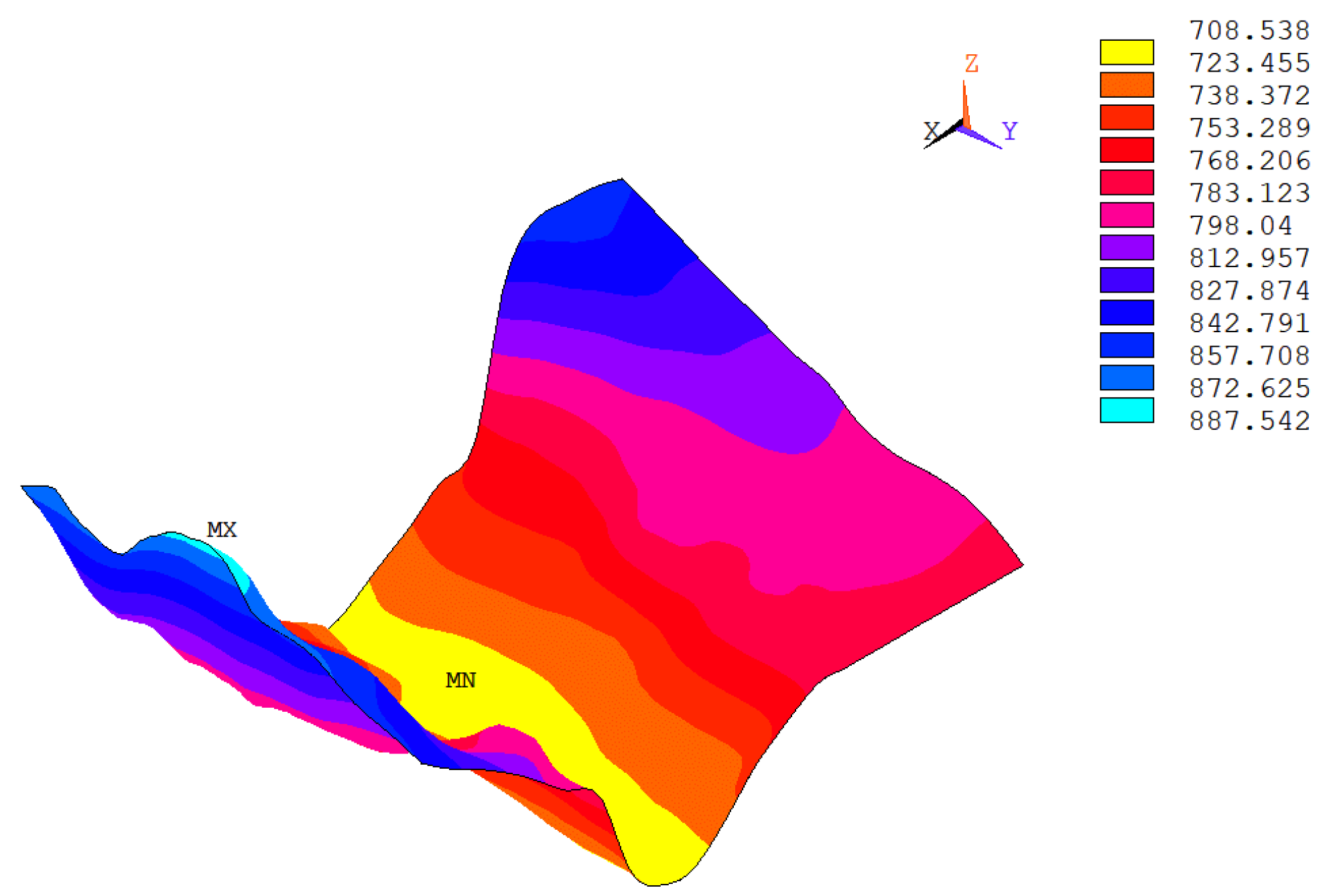
The DEM was obtained applying the methodology explained in this article. The same finite element program used for the stress–strain calculation of the structure was used to create the DEM. From a base of 13 × 21 points and a finite element mesh of 4000 nodes, the terrain topography was created and included in the model (with the resulting DEM shown in Figure 2).
Note that the original regular mesh (eight node brick elements) is maintained in the model that includes the DEM. No mesh modification was done apart from moving the nodes in the vertical position. This has great significance in finite element models, where the regularity of the mesh is an important factor regarding its accuracy. The presented methodology allows this to be done in a very simple way.
In addition to proposing the methodology and analyzing the factors that influence the results obtained, the procedure is illustrated with examples to analyze the validity of the method in a particular case.

2. Methodology

Our aim is to define a digital elevation model from a set of stake out points.
The application of the proposed methodology is very simple and can be summarized in the following steps:
  • Locate the set of known points within the domain (horizontal coordinates).
  • Mesh the domain.
  • Apply boundary conditions.
  • Solve the finite element model.
As explained later, to obtain the best results, it is recommended to have a mesh that is as uniform as possible (all elements with approximately the same size).

2.1. Thin Plate Formulation

Finite element models are a well known technique [7] for numerically solving differential equations that appear in many engineering fields such as structural analysis, fluids, thermal analysis, electromagnetism, etc. The terrain to be obtained is represented by a three-dimensional surface, which is discretized using shell elements. The idea behind this approach can be regarded as metal stamping. In this case, the product is the final DEM and the mold/press is set by the boundary conditions applied to the plate. The plate must change its shape to adapt to the mold.
The terrain is mapped to a plate on which a series of imposed movements take place. These imposed movements are the elevations of the known terrain points, and the resulting movements in the rest of the nodes of the plate are the elevations of different terrain points.
Different approaches can be followed, but the one chosen here is to use the thin plate formulation or Kirchhoff plate theory [8,9]; for a plate with a constant thickness and isotropic material, this is given by
4 w x 4 + 2 4 w x 2 y 2 + 4 w y 4 = q D
This can be expressed in a compact form as
4 w = q D
The finite element method is based on the well-known equation that relates the array of movements u to the array of applied forces P through the stiffness matrix K :
Ku = P
The stiffness matrix is defined as
K i j = A B i T C f B j d a
where
B i = 2 φ i x 2 2 φ θ x i x 2 2 φ θ y i x 2 2 φ i y 2 2 φ θ x i y 2 2 φ θ y i y 2 2 2 φ i x y 2 2 φ θ x i x y 2 2 φ θ y i x y
and
C f = D 1 ν 0 ν 1 0 0 0 1 ν 2
where φ i are the form functions for the displacements (out of plane), and φ θ x i , φ θ y i are the function forms for the rotations. ν is the Poisson’s ratio, and its influence can be seen later.
The thin plate formulation is implemented in nearly all the finite element programs, and its formulation is simple enough to provide a quick solution, even for large meshes.
Other approaches could have been followed, such as using the Mindlin–Reissner plate theory [9] (shell elements) or meshing the terrain using brick elements in one or several layers. These ideas were disregarded once the thin plate approach was tested, as the results provided were good enough and there was no need to increase the complexity of the model.
As has been pointed out, the FEM is used as a numerical tool with which an abstraction has been done to obtain the topographical coordinates of the points of a terrain as the movements of the points on a plate. There are many publications in which a similar concept is used, using the FEM as a support numerical tool [10,11]. The concept of the exposed methodology could also be translated to a different numerical method (i.e., finite differences method [12], generalized finite differences method [13,14], discrete element method [15], etc.), but the FEM was chosen because it is the most used method in civil engineering software. In addition a different approach could be chosen using the heat transfer theory or a more general elastic theory, but again, the Kirchhoff plate theory was used due to its simple and normal implementation in civil engineering software.

2.2. Domain Definition

There is no special rule to establish the domain, apart from the obvious condition that all the stake out points should be within the domain. The domain may have any shape, and there is no need to have stake out points at the boundaries of the domain.

2.3. Meshing of the Domain

This is one of the most critical parts of the methodology. The domain must be meshed, but the stake out points must be exactly represented as nodes of the mesh. To do so, several approaches are given, all of which valid, but some will be of preferential use depending on the meshing software to be used.
The generality of the method allows meshing to be performed with any kind of element (three nodes, four nodes, etc.). It is important to take into account that the mesh used to define the DEM (as described in this chapter) does not need to match the one used in the FEM of the structure. This is to say, if the same software is used to model the structure and the DEM, different meshes can be used. Nevertheless, if the mesh used for the DEM includes the same node locations (or geometry) as the one employed for the structure, the translation of the DEM to the structure FEM will be straightforward, without the need to interpolate (see Figure 1).
Once this is clarified, some guidelines to create a good mesh are given hereafter, which may be applied to a completely new mesh or a mesh based on the FEM model of the structure:
  • Displacement of nodes on a generic mesh,
  • Subdivision of the domain,
  • Remeshing.

2.3.1. Generic Meshing and Displacement of Nodes

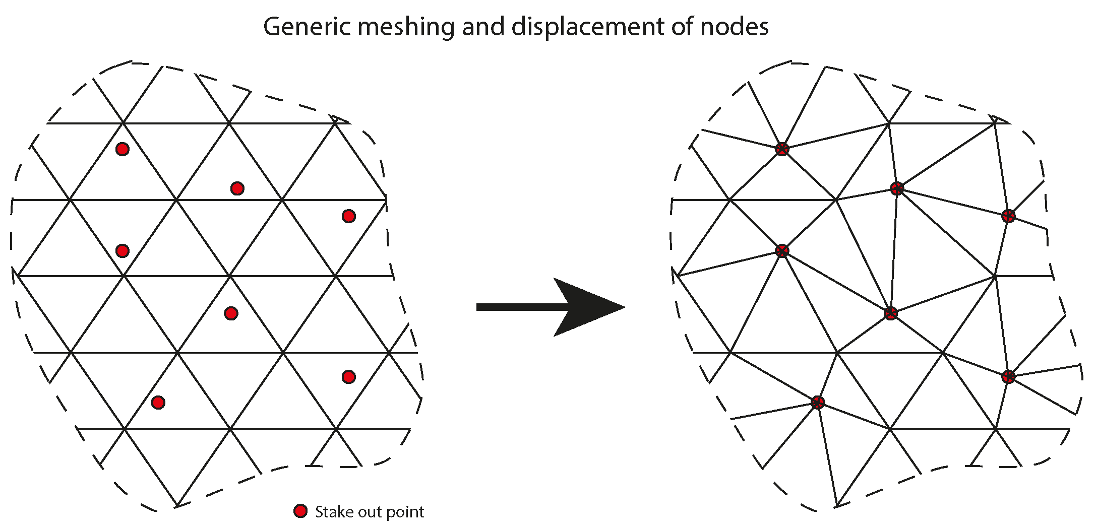
A completely generic mesh can be generated and then adapted to the stake out points by moving the nearest points (Figure 3).
If the mesh is coarse, this option is not recommended as it may lead to distorted elements.

2.3.2. Subdivision of the Domain

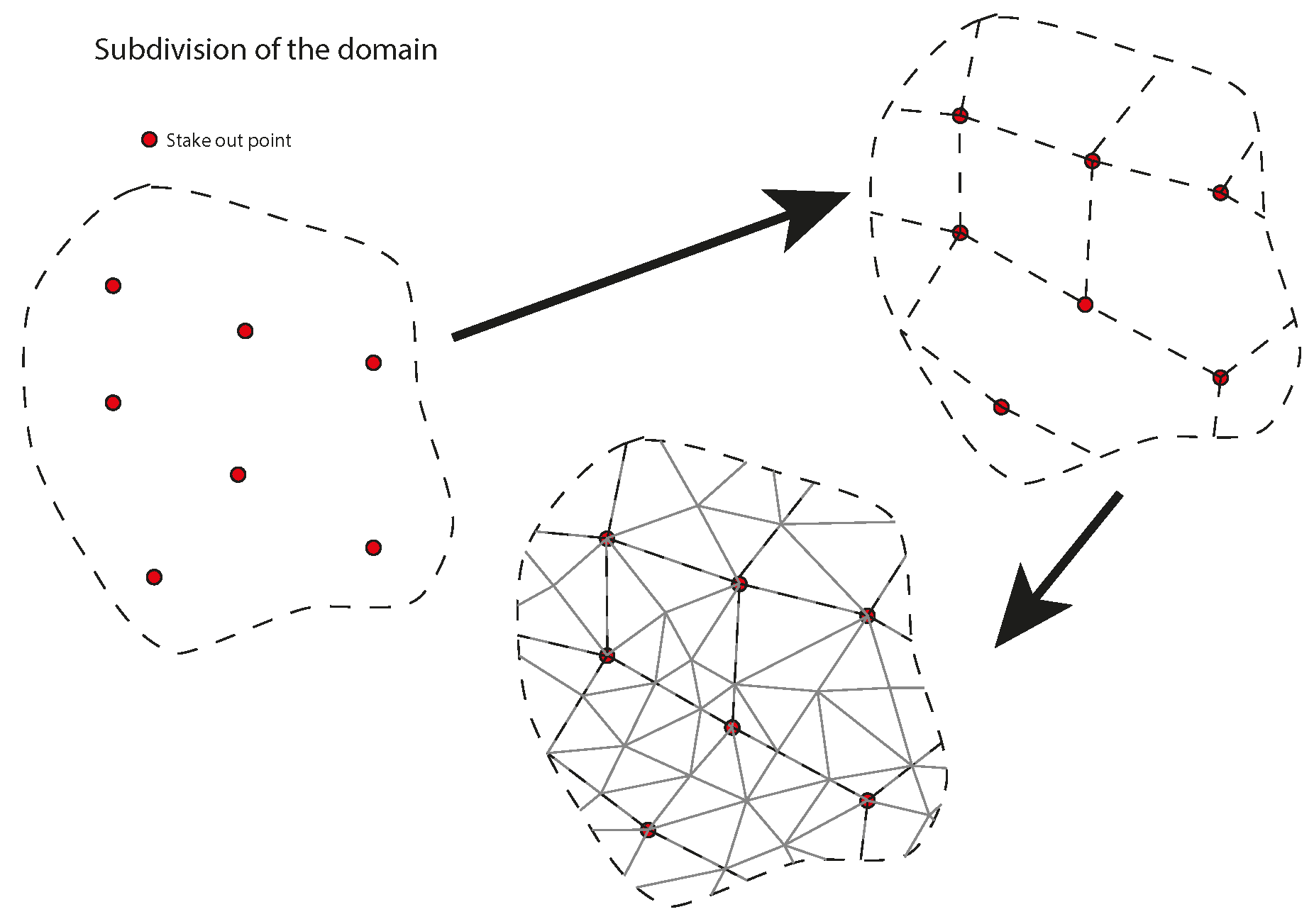
In this approach, the domain is divided into subdomains by conducting a triangulation of the initial domain using the stake out points as vertices of the triangulation. Then, the subdomains are meshed, imposing continuity on the mesh at the boundaries between subdomains (Figure 4).
This procedure is easy to implement and gives good results if the mesh is not too coarse; otherwise, the boundaries between subdomains will establish false hips or valleys on the digital elevation model.

2.3.3. Remeshing

Another valid option, based on the first, is to create a free mesh on the domain and then break the elements onto which the stake out points fall on into smaller elements with the stake out point as a node (Figure 5). This leads to smaller elements around the stake points, which is not the optimum choice, so a recommended procedure is to create an initial coarse mesh, break the elements to fit the stake out points and then remesh the rest of the elements (subdivide them) to match the sizes of all elements.

2.4. Boundary Conditions

The boundary conditions of the finite element model are given by the stake out points: all the nodes at the stake out points will have a fixed vertical displacement, equal to the height of the corresponding stake out point. Additionally, to restrain the model to be solved, two arbitrary nodes will have one of the horizontal displacements fixed, and one arbitrary node will have the other of the horizontal displacement fixed. The boundaries of the model need not to be restrained or fixed in any way, and the model has no concentrated, surface or body forces applied.

3. Influence of Material Parameters

The model must be defined using a unique material.
As can be seen from finite element exposition for the thin plane formulation, the thickness of the plate and the elasticity modulus have no effect on the solution (they are a constant out of the integral that scales the stresses, but the overall deformed shape remains the same).
Nevertheless, this is not the case for the Poisson ratio, which will have an influence on the deformed shape and how this adapts to the given set of points.

4. Verification Examples

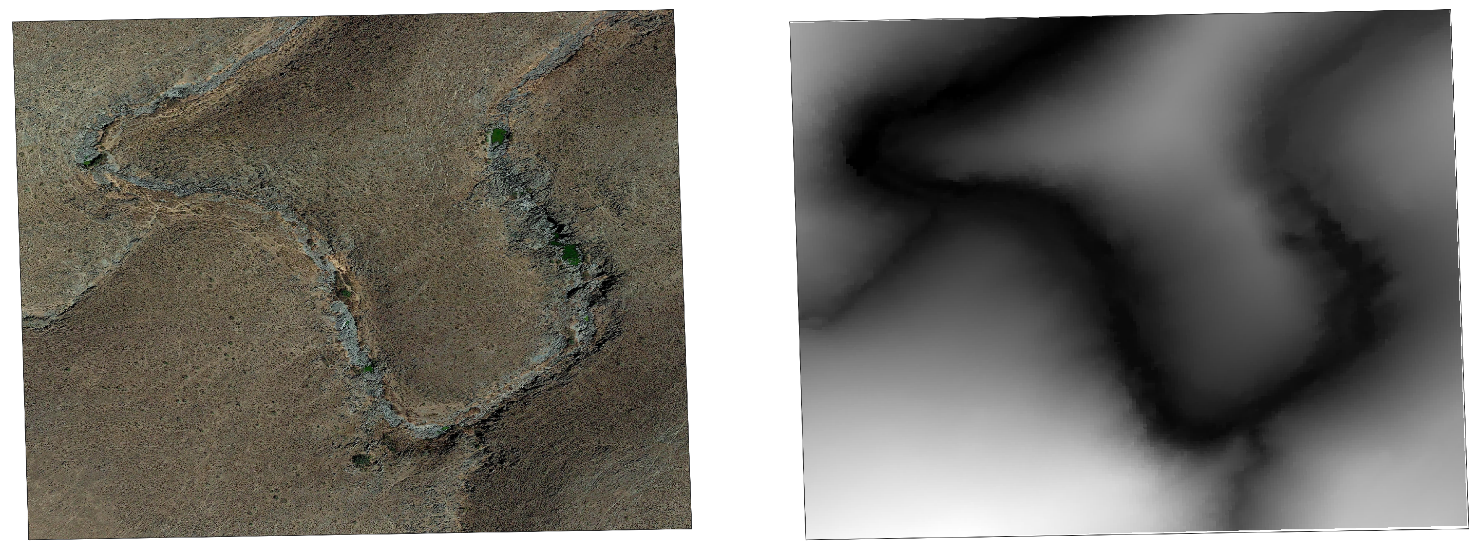
The model used is part of the MDT02 2019 CC-BY 4.0 Instituto Geográfico Nacional (Spanish National Geographic Institute). It is a steep area with a river characterized by sharp meanders (Figure 6).
The stake out points have been chosen in two ways:
  • As a regular mesh (equidistant) and
  • Randomly distributed.
For the modeling, the software Ansys®Academic Research Mechanical, Release 21.1 has been used [16,17,18].
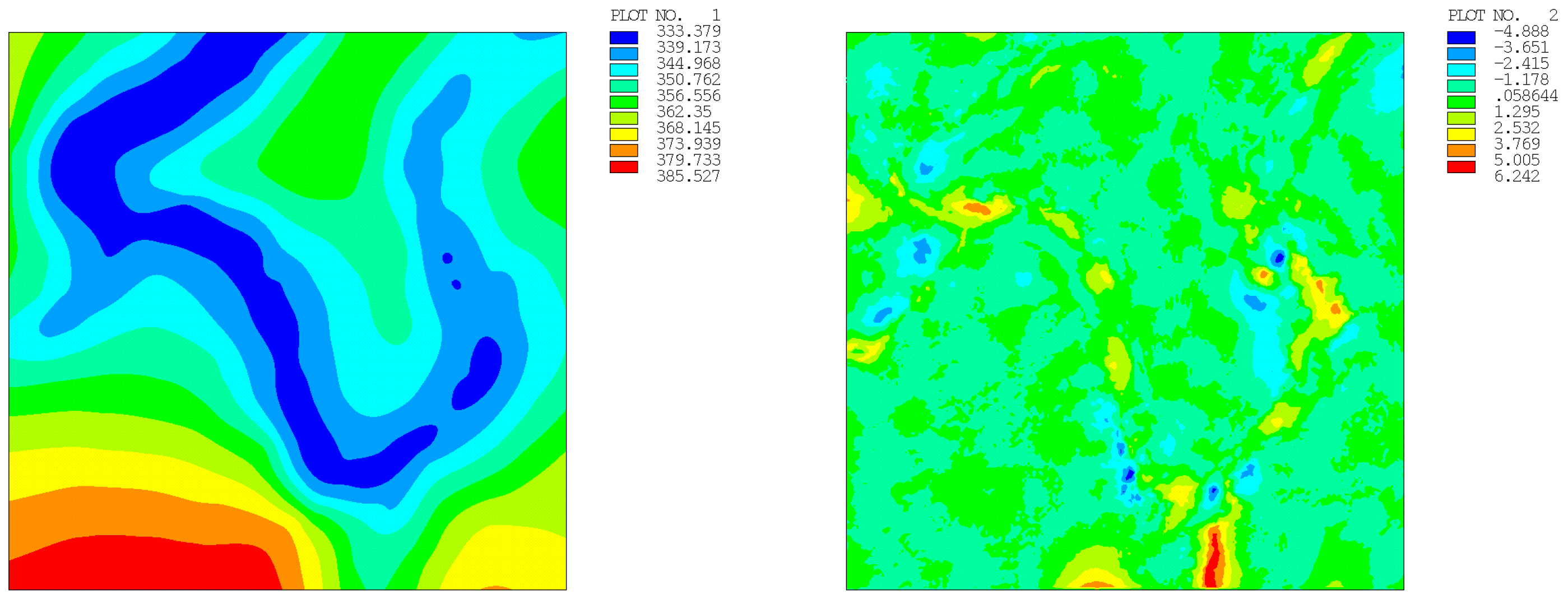
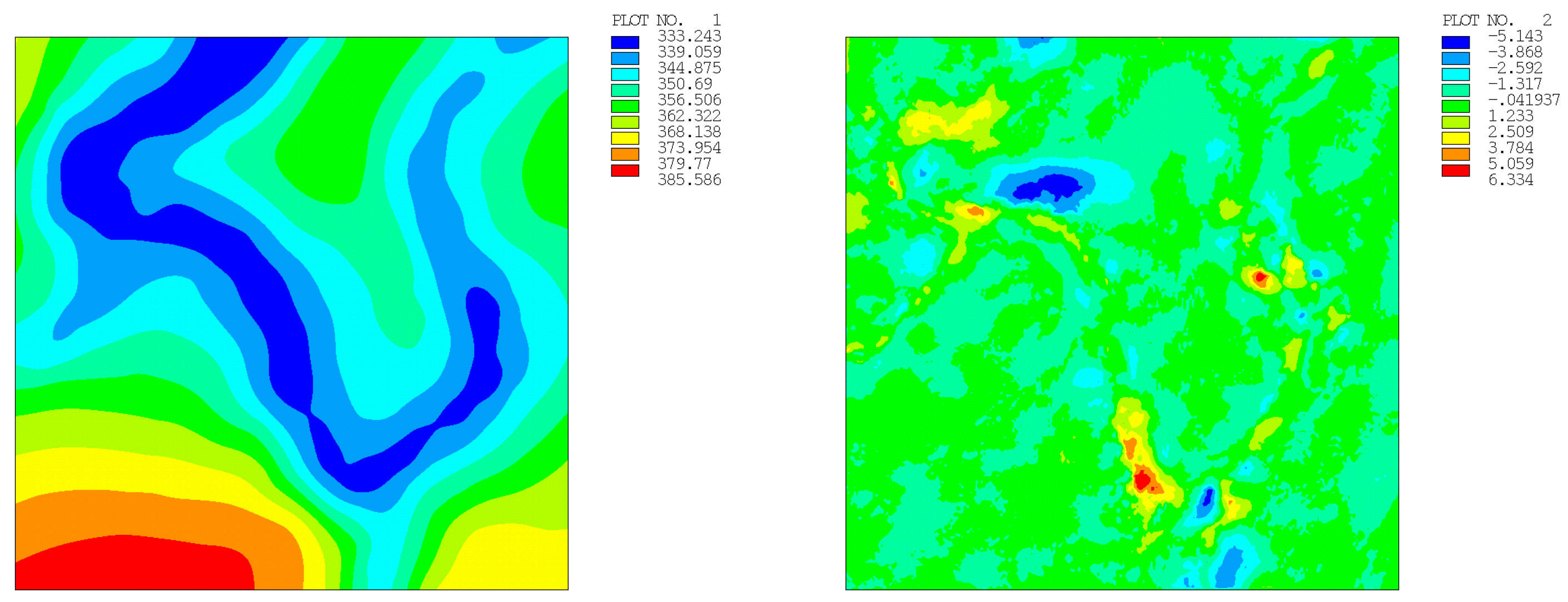
In both cases, several examples have been run, with different numbers of stake out points: 49, 100, 196 and 400. For the case of a random distribution, each of the examples has been run three times with a different seed for the generation of the random points. In conclusion, a total of 16 runs have been made.
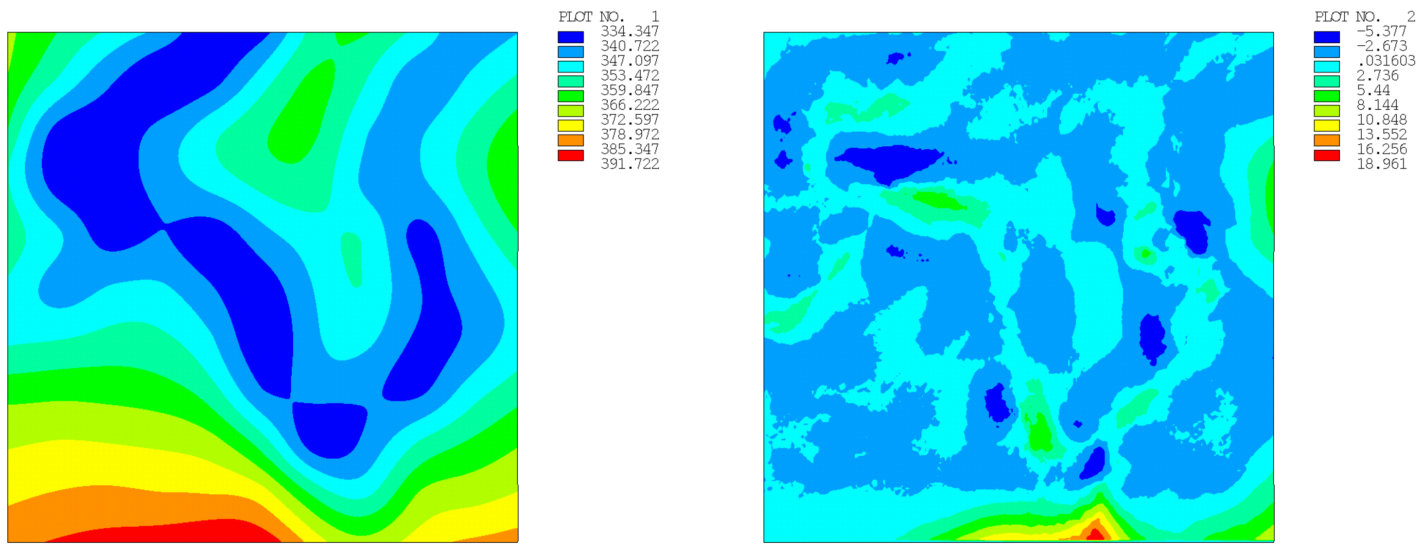
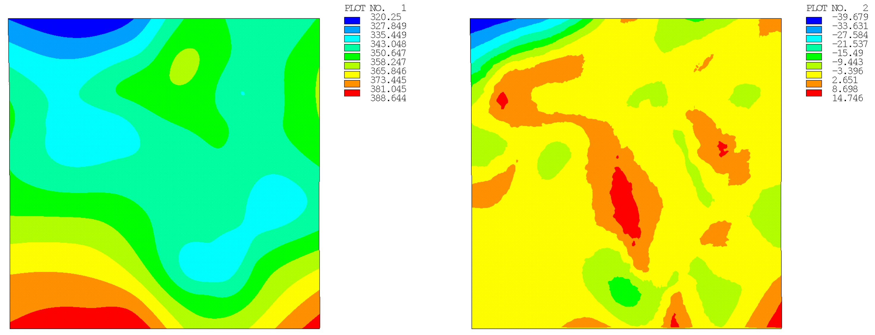
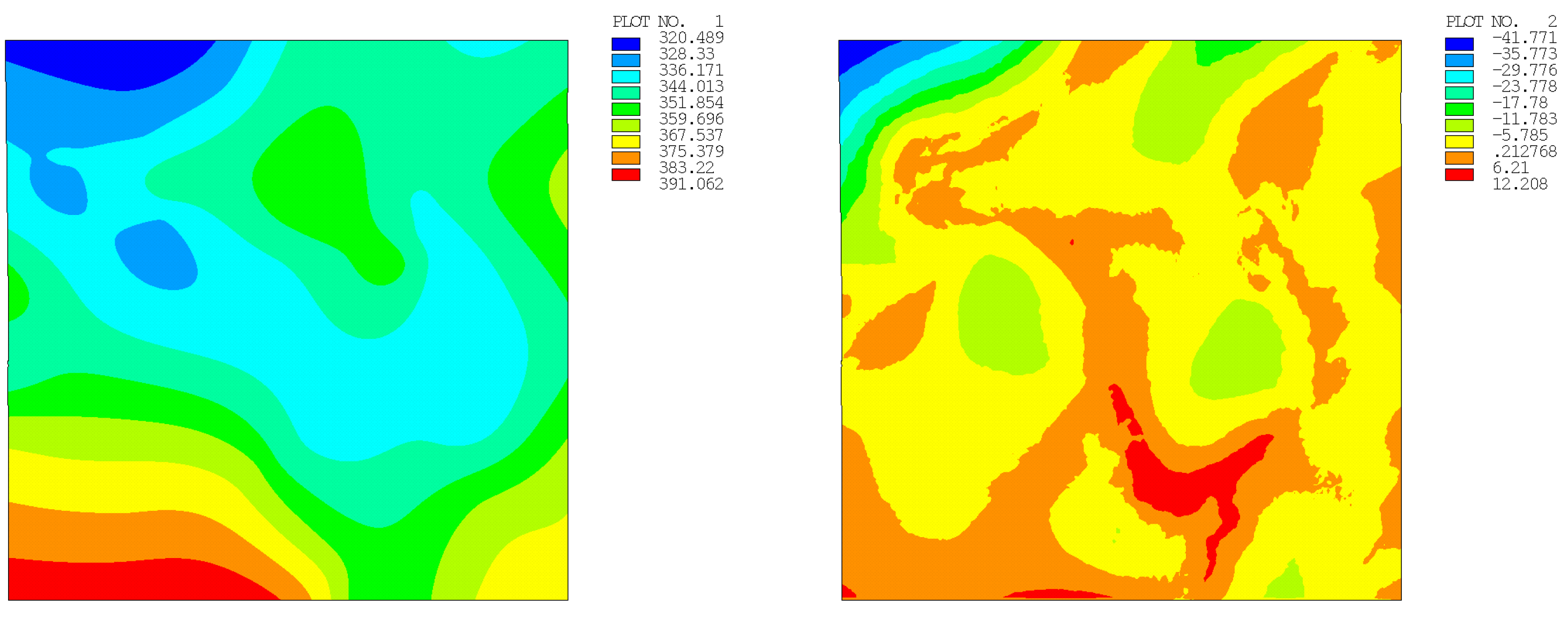
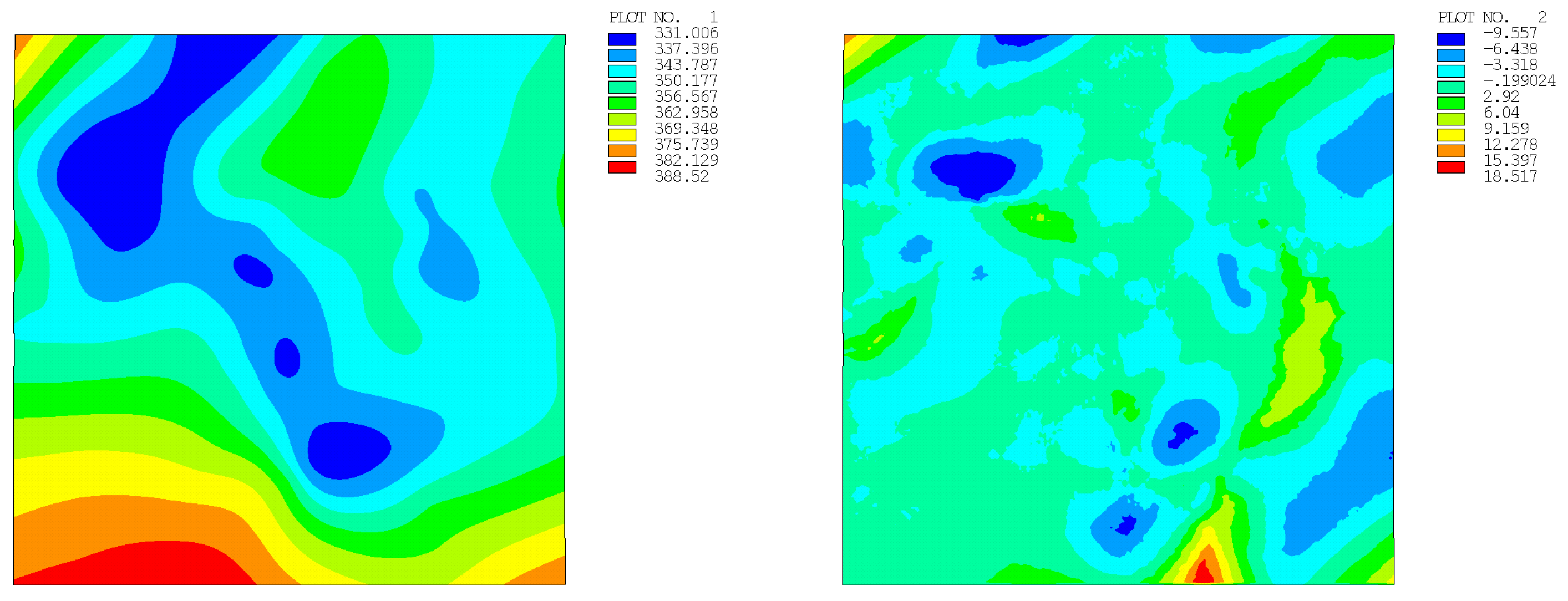
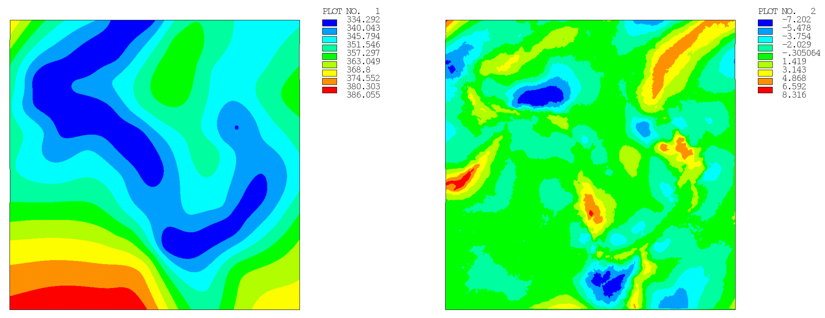
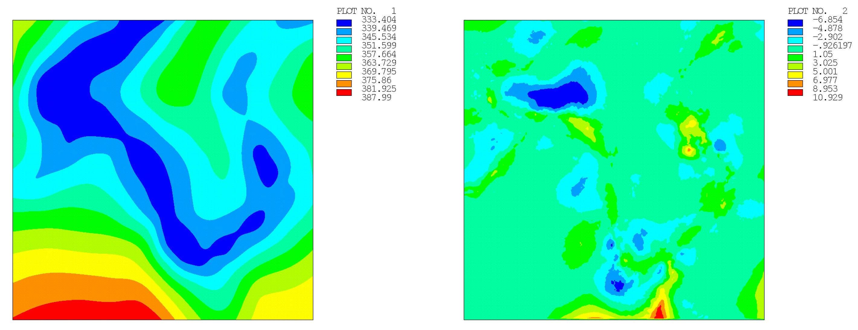
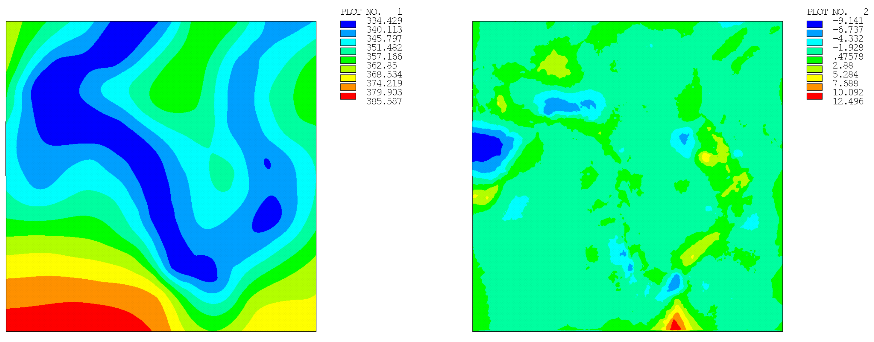
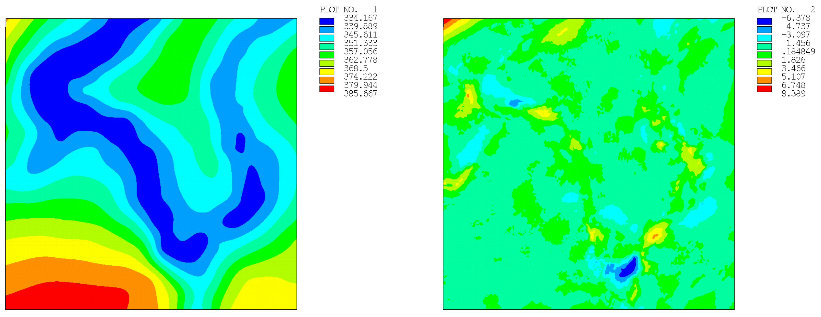
The results are shown hereafter (Figure 7, Figure 8, Figure 9, Figure 10, Figure 11, Figure 12, Figure 13, Figure 14, Figure 15, Figure 16, Figure 17, Figure 18, Figure 19, Figure 20, Figure 21 and Figure 22). The image on the left shows the obtained DEM, and the image on the right shows the differences contour plot, where the difference is obtained as the obtained height minus the height of the high-resolution DEM. Obviously, this cannot be treated as an error in the methodology but can give an idea of how the methodology adapts a plane surface to a topographical surface, with the smoothness of the slopes compared to the ones found in a typical landscape, etc.
Table 1 summarizes the maximum differences obtained (in meters). The value in parentheses is the mean difference over the entire surface.
Abnormal results are obtained for the random distributions with 49 and 100 points and seed 3: the maximum difference is lower than for the other seeds, and that for 100 points is indeed lower than for 196 points. This is due to the particular point distribution obtained by the random generation and is the reason why 3 seeds where considered in each case in order to obtain an overall picture.
As can be seen, the maximum differences are obtained in the areas with greater slopes (height gradients) or at the corners. Obviously, a human-chosen cloud of points, instead of an artificial (regular or random) set of points, would reduce the difference and increase the accuracy.
A different example has been developed in order to analyze the influence of the Poisson’s ratio over the results. Taking the regular distribution with 196 points, the Poisson ratio has been varied in order to see its influence. The results are shown in Figure 23. As can be seen, the maximum difference decreases as the Poisson ratio increases, while the average difference remains stable. Nevertheless, the decrease in the difference is not very significant (5% comparing η = 0.05 with η = 0.30 ).
The code that reproduces the example of the 49 points models with random generation is provided in Appendix A. It is written for ANSYS APDL.

5. Real Case Example

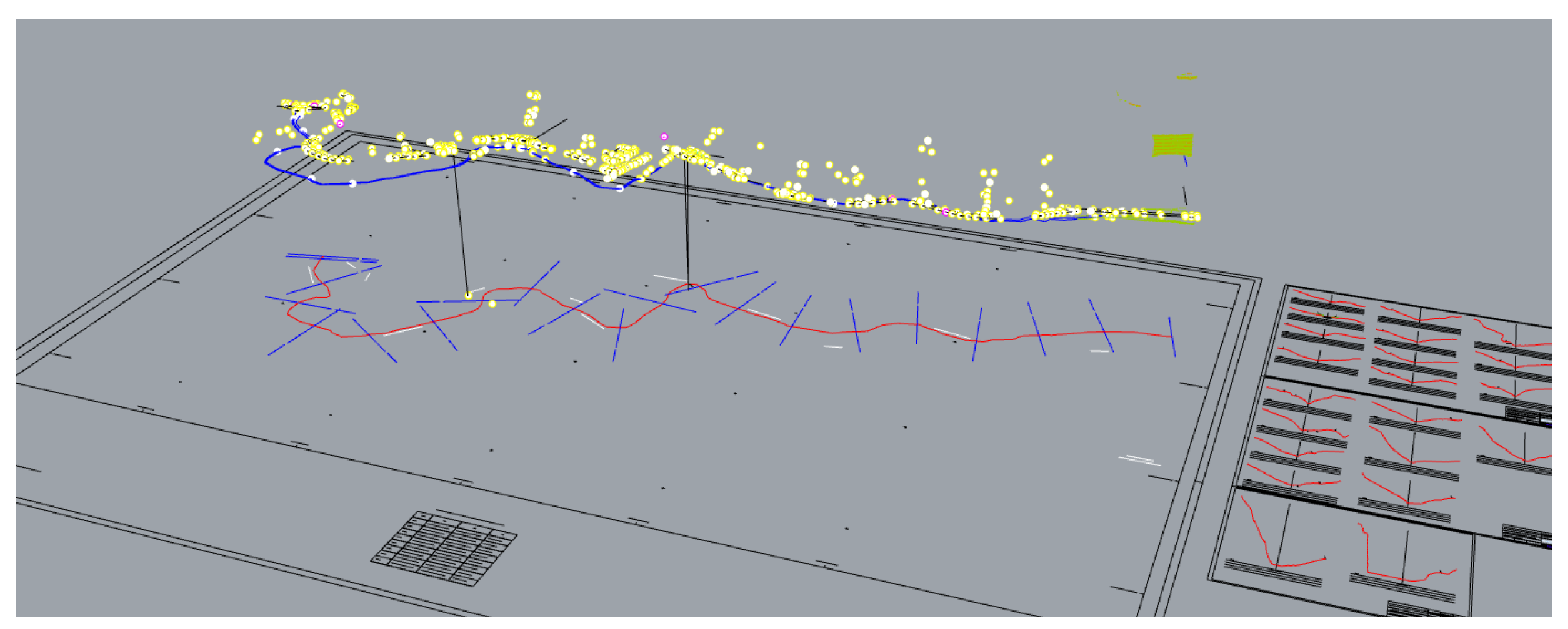
The methodology has been applied to a real case, where the topographic surface of a river was to be obtained from a series of measured points. Figure 24 shows a representation of the measured points over the plan view of the river, representing its real height (in perspective). The number of points is not large, as they have not been obtained from a LiDAR scan. On the other hand, they are not placed following a regular pattern, but on the contrary, they are distributed in a completely irregular way.
The DEM generated from the FEM procedure is shown in Figure 25, and its representation along with the measured points is shown in Figure 26.
It can be seen that the approximation from the given points is good. The generated surface has the required smoothness, without mathematical artifacts.

6. Discussion

The shown methodology represents an alternative way to obtain a vector-based network DTM given a group of stake out points. The methodology is developed throughout the article, and advice on its application is given.
The DTM has the particularity that only one point can occupy the same horizontal coordinates. Therefore, the proposed methodology is not valid for any general three-dimensional surface. What makes this methodology especially useful is the fact that it is applicable when only a small number of points (several tens or a few hundred) are available.
Without being the most accurate procedure published to date, our approach is characterized by being a very simple way to approach and solve the problem and by making use of tools already found within the software used in civil engineering offices.
Moreover, the procedure allows the DTM to be obtained inside only the finite element software used to analyze a structure (bridge, dam, tunnel, etc.), simplifying the process of importing or interpreting external geometry. The original mesh can be used as well, and so in order to adapt the original mesh of the structure, no complex mesh modification has to be done apart from moving the nodes in the vertical position.
Focusing on the accuracy of the method, as said before, it is not one of the most accurate approaches as it fails to distinguish plains from steep areas, etc., but the accuracy obtained is sufficient for the representation of the terrain in a finite element model. The methodology obtains a smooth DEM that represents the terrain as accurately as the number of points given and their location allow (if chosen wisely, the DEM can be very accurate).
The use of shell elements makes it available for nearly any FEM software and provides a solution that is very fast without complex calculations. The only parameter that defines the shell elements, which may change the results, is the Poisson ratio, but as has been shown, its influence is not very important.
The procedure could also be used with a different numerical method (i.e., finite differences method, generalized finite differences method, discrete element method, etc.) where the structural plate theory is modeled, but the FEM was chosen because it is the most used method in civil engineering software. In addition, a different approach could be chosen using the heat transfer theory or a more general elastic theory, but again, the Kirchhoff plate theory was used due to its simple and normal implementation in civil engineering software.

Author Contributions

Conceptualization, E.C.L., E.S.C. and J.F.E.; Data curation, E.C.L. and E.S.C.; Formal analysis, A.V.U.; Investigation, E.C.L., E.S.C., J.F.E. and A.V.U.; Methodology, E.C.L., E.S.C. and J.F.E.; Project administration, E.S.C.; Resources, E.C.L. and A.V.U.; Software, E.S.C.; Validation, J.F.E. and A.V.U.; Visualization, E.C.L. and E.S.C.; Writing—original draft, E.C.L., E.S.C. and A.V.U.; Writing—review and editing, E.C.L., E.S.C., J.F.E. and A.V.U. All authors have read and agreed to the published version of the manuscript.

Funding

A. Vargas Ureña acknowledges financial support from the Spanish Ministerio de Ciencia e Innovación (grant FJC2021-046953-I).

Institutional Review Board Statement

Not applicable.

Data Availability Statement

No new data were created or analyzed in this study. Data sharing is not applicable to this article.

Conflicts of Interest

The authors declare no conflict of interest.

Abbreviations

    The following abbreviations are used in this manuscript:
FEMFinite element model
DEMDigital elevation model
DTMDigital terrain model
LiDARLaser Imaging Detection and Ranging
CADComputer aided design

Appendix A. Sample Code

Below is the code used to create one of the examples shown in the article. To simplify the code, the included example has a low number of points, although the code is perfectly applicable to any of the other models, simply by increasing the number of points.
The example is one of the models with a random generation of 49 points.
The code is written in ANSYS APDL.
FINISH
/CLEAR
/PREP7
n = 200
paso = 2 ! meters
ET,1,63
MP,EX,1,1E6
MP,NUXY,1,0.30
R,1,0.20
*DO,II,1,n
*DO,JJ,1,n
  N,II+10000*JJ,paso*(JJ-1),paso*(II-1),0.0
*ENDDO
*ENDDO
*DO,II,1,n-1
*DO,JJ,1,n-1
  E,II+10000*JJ,II+1+10000*JJ,II+1+10000*(JJ+1),II+10000*(JJ+1)
*ENDDO
*ENDDO
NPoints = 49
Points =
*DIM,Points,ARRAY,3,49
Points(1,1)=296,304,343.118
Points(1,2)=8,18,380.344
Points(1,3)=140,304,351.327
Points(1,4)=316,84,350.611
Points(1,5)=110,126,361.273
Points(1,6)=240,12,359.673
Points(1,7)=136,210,344.65
Points(1,8)=168,374,337.083
Points(1,9)=92,302,343.349
Points(1,10)=268,84,337.506
Points(1,11)=346,392,344.677
Points(1,12)=148,282,346.736
Points(1,13)=328,352,345.978
Points(1,14)=332,266,346.912
Points(1,15)=176,324,353.751
Points(1,16)=348,16,371.539
Points(1,17)=14,270,349.119
Points(1,18)=358,344,351.089
Points(1,19)=36,260,344.047
Points(1,20)=274,262,351.477
Points(1,21)=104,352,334.844
Points(1,22)=392,212,350.687
Points(1,23)=242,82,336.557
Points(1,24)=266,184,350.626
Points(1,25)=12,122,363.053
Points(1,26)=258,108,342.424
Points(1,27)=280,56,345.087
Points(1,28)=340,158,337.234
Points(1,29)=354,114,349.082
Points(1,30)=226,218,346.505
Points(1,31)=132,254,337.66
Points(1,32)=220,346,359.826
Points(1,33)=156,26,380.108
Points(1,34)=254,44,350.323
Points(1,35)=282,352,351.043
Points(1,36)=344,262,349.513
Points(1,37)=26,54,376.473
Points(1,38)=44,254,343.468
Points(1,39)=314,320,345.781
Points(1,40)=174,346,347.06
Points(1,41)=80,16,383.246
Points(1,42)=110,18,382.844
Points(1,43)=72,242,339.45
Points(1,44)=282,138,345.909
Points(1,45)=18,116,364.61
Points(1,46)=370,202,346.298
Points(1,47)=362,40,369.266
Points(1,48)=70,240,339.433
Points(1,49)=284,100,337.055
*DO,II,1,NPoints
  ThisNode = Node(Points(1,II),Points(2,II),0)
  D,ThisNode,UZ,Points(3,II)
*ENDDO
D,1+10000,UX,0
D,2+10000,UX,0
D,1+10000,UY,0
/SOLU
SOLVE

References

  1. Southard, D. Piecewise Planar Surface Models from Sampled Data. In Scientific Visualization of Physical Phenomena; ch. 11.5; Springer: Berlin/Heidelberg, Germany, 1991. [Google Scholar]
  2. Feciskanin, R.; Minár, J. Polygonal Simplification and Its Use in DEM Generalization for Land Surface Segmentation. Trans. Gis 2021, 25, 2361–2375. [Google Scholar] [CrossRef]
  3. Sun, W.; Wang, H.; Zhao, X. A simplification method for grid-based DEM using topological hierarchies. Surv. Rev. 2018, 50, 454–467. [Google Scholar] [CrossRef] [Green Version]
  4. Zhu, D.; Cheng, X.; Zhang, F.; Yao, X.; Gao, Y.; Liu, Y. Spatial interpolation using conditional generative adversarial neural networks. Int. J. Geogr. Inf. Sci. 2020, 34, 735–758. [Google Scholar] [CrossRef]
  5. Alzaghoul, E.; Al-Zoubi, M.B.; Obiedat, R.; Alzaghoul, F. Applying Machine Learning to DEM Raster Images. Technologies 2021, 9, 87. [Google Scholar] [CrossRef]
  6. Podobnikar, T.; Vrečko, A. High Quality DEM from LiDAR Data. Trans. Gis 2012, 16, 603–617. [Google Scholar] [CrossRef]
  7. Bathe, K.J. Finite Element Procedures; Klaus-Jurgen Bathe: USA, 2006; ISBN 097900490X. [Google Scholar]
  8. Benito, J.J.; Álvarez, R.; Ureña, F.; Salete, E.; Aranda, E. Introduction to Finite Element Method; Editorial UNED: Madrid, Spain, 2014; ISBN 978-84-362-6752-5. [Google Scholar]
  9. Ahmad, S.; Irons, B.M.; Zienkiewicz, O.C. Analysis of Thick and Thin Shell Structures by Curved Finite Elements. Int. J. Numer. Methods Eng. 1970, 2, 419–451. [Google Scholar] [CrossRef]
  10. Sharma, D.; Jiwari, R.; Kumar, S. Numerical Solution of Two Point Boundary Value Problems Using Galerkin-Finite Element Method. Int. J. Nonlinear Sci. 2012, 13, 204–210. [Google Scholar]
  11. Ankur; Jiwari, R.; Kuma, N. Analysis and simulation of Korteweg-de Vries-Rosenau-regularised long-wave model via Galerkin finite element method. Comput. Math. Appl. 2023, 135, 134–148. [Google Scholar] [CrossRef]
  12. Mitchell, A.R.; Griffiths, D.F. The Finite Difference Method in Partial Differential Equations; John Wiley & Sons: Hoboken, NJ, USA, 1980; ISBN 041727641. [Google Scholar]
  13. Liszka, T.; Orkisz, J. The finite difference method at arbitrary irregular grids and its application in applied mechanics. Comput. Struct. 1980, 11, 83–95. [Google Scholar] [CrossRef]
  14. Benito, J.J.; Ureña, L.F. Gavete, Influence of several factors in the generalized finite difference method. Appl. Math. Model. 2001, 25, 1039–1053. [Google Scholar] [CrossRef]
  15. Peng, Z.; Doroodchi, E.; Moghtaderi, B. Heat transfer modelling in Discrete Element Method (DEM)-based simulations of thermal processes: Theory and model development. Prog. Energy Combust. Sci. 2020, 79, 100847. [Google Scholar] [CrossRef]
  16. Ansys®Academic Research Mechanical APDL. Release 2022 R1, Help System, Theory Reference; ANSYS, Inc.: USA, 2022. [Google Scholar]
  17. Ansys®Academic Research Mechanical APDL. Release 2022 R1, Structural Analysis Guide, Theory Reference; ANSYS, Inc.: USA, 2022. [Google Scholar]
  18. Ansys®Academic Research Mechanical APDL. Release 2022 R1, Modeling and Meshing Guide, Theory Reference; ANSYS, Inc.: USA, 2022. [Google Scholar]
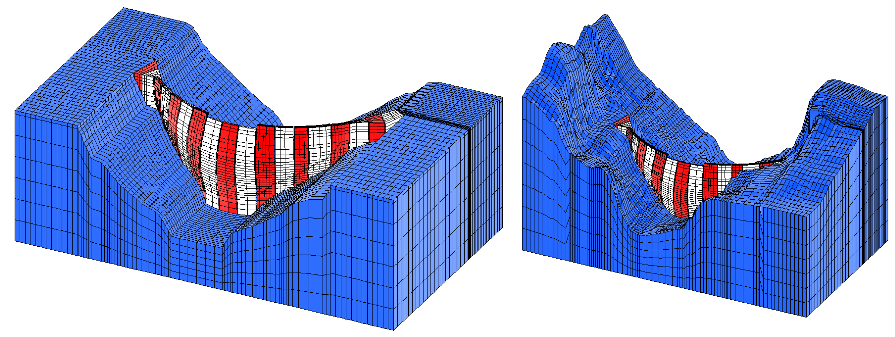
Figure 1. Finite element model of a dam. Initial model without DEM (left) and final model with DEM (right). View from upstream, right riverbank.
Mathematics 11 01522 g001
Figure 2. Real case obtained with DEM. View from upstream, left riverbank.
Mathematics 11 01522 g002
Figure 3. Generic meshing and displacement of nodes.
Mathematics 11 01522 g003
Figure 4. Subdivision of the domain.
Mathematics 11 01522 g004
Figure 5. Remeshing of the domain. (Up): Remesh only elements where stake out points fall. (Down): Coarse mesh and remesh all elements.
Mathematics 11 01522 g005
Figure 6. (Left): Satellite photograph of the terrain. (Right): Original DEM.
Mathematics 11 01522 g006
Figure 7. Regular mesh 49 points. (Left): DEM. (Right): Difference with high-res DEM.
Mathematics 11 01522 g007
Figure 8. Regular mesh 100 points. (Left): DEM. (Right): Difference with high-res DEM.
Mathematics 11 01522 g008
Figure 9. Regular mesh 196 points. (Left): DEM. (Right): Difference with high-res DEM.
Mathematics 11 01522 g009
Figure 10. Regular mesh 400 points. (Left): DEM. (Right): Difference with high-res DEM.
Mathematics 11 01522 g010
Figure 11. Random 49 points (seed 1). (Left): DEM. (Right): Difference with high-res DEM.
Mathematics 11 01522 g011
Figure 12. Random 49 points (seed 2). (Left): DEM. (Right): Difference with high-res DEM.
Mathematics 11 01522 g012
Figure 13. Random 49 points (seed 3). (Left): DEM. (Right): Difference with high-res DEM.
Mathematics 11 01522 g013
Figure 14. Random 100 points (seed 1). (Left): DEM. (Right): Difference with high-res DEM.
Mathematics 11 01522 g014
Figure 15. Random 100 points (seed 2). (Left): DEM. (Right): Difference with high-res DEM.
Mathematics 11 01522 g015
Figure 16. Random 100 points (seed 3). (Left): DEM. (Right): Difference with high-res DEM.
Mathematics 11 01522 g016
Figure 17. Random 196 points (seed 1). (Left): DEM. (Right): Difference with high-res DEM.
Mathematics 11 01522 g017
Figure 18. Random 196 points (seed 2). (Left): DEM. (Right): Difference with high-res DEM.
Mathematics 11 01522 g018
Figure 19. Random 196 points (seed 3). (Left): DEM. (Right): Difference with high-res DEM.
Mathematics 11 01522 g019
Figure 20. Random 400 points (seed 1). (Left): DEM. (Right): Difference with high-res DEM.
Mathematics 11 01522 g020
Figure 21. Random 400 points (seed 2). (Left): DEM. (Right): Difference with high-res DEM.
Mathematics 11 01522 g021
Figure 22. Random 400 points (seed 3). (Left): DEM. (Right): Difference with high-res DEM.
Mathematics 11 01522 g022
Figure 23. Difference vs Poisson ratio.
Mathematics 11 01522 g023
Figure 24. Real case of a river bed. Measured points shown in perspective over the plan view.
Mathematics 11 01522 g024
Figure 25. Real case of a river bed. DEM generated from the FEM model.
Mathematics 11 01522 g025
Figure 26. Real case of a river bed. DEM generated in perspective with the measured points.
Mathematics 11 01522 g026
Table 1. Maximum and mean (in parentheses) differences for each example.
Number of PointsRegular DistributionRandom Distribution
Seed 1Seed 2Seed 3
4925.365 (2.790)39.838 (3.573)41.930 (3.785)17.980 (2.816)
10018.961 (1.279)18.517 (1.885)18.114 (1.768)8.316 (1.397)
19614.162 (0.762)11.058 (1.011)10.929 (0.984)12.496 (0.938)
4004.857 (0.344)8.389 (0.582)6.242 (0.512)6.334 (0.537)
Disclaimer/Publisher’s Note: The statements, opinions and data contained in all publications are solely those of the individual author(s) and contributor(s) and not of MDPI and/or the editor(s). MDPI and/or the editor(s) disclaim responsibility for any injury to people or property resulting from any ideas, methods, instructions or products referred to in the content.