Author Contributions
Conceptualization, A.L.C., R.A.G. and J.C.A.; methodology, A.L.C. and J.C.A.; software, A.L.C.; validation, R.C. and B.I.G.; formal analysis, A.L.C., R.A.G., R.C., B.I.G. and J.C.A.; investigation, A.L.C., R.A.G. and J.C.A.; resources, J.C.A.; writing—original draft preparation, A.L.C., R.A.G., R.C., B.I.G. and J.C.A.; writing—review and editing, A.L.C., R.C., B.I.G. and J.C.A.; visualization, R.C. and B.I.G.; supervision, J.C.A. All authors have read and agreed to the published version of the manuscript.
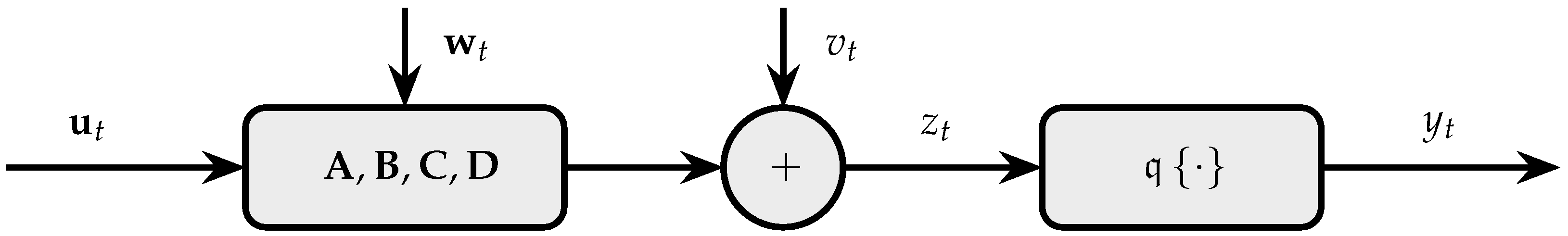
Figure 1.
State-space model with quantized output.
Figure 1.
State-space model with quantized output.
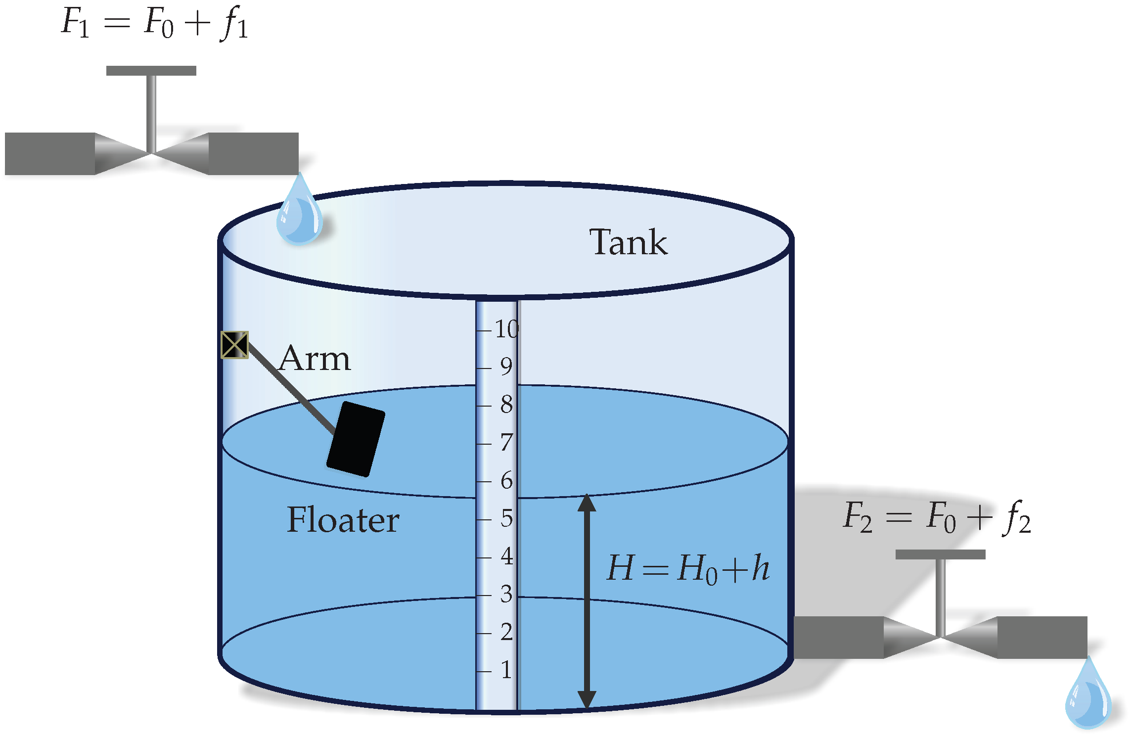
Figure 2.
Liquid-level system.
Figure 2.
Liquid-level system.
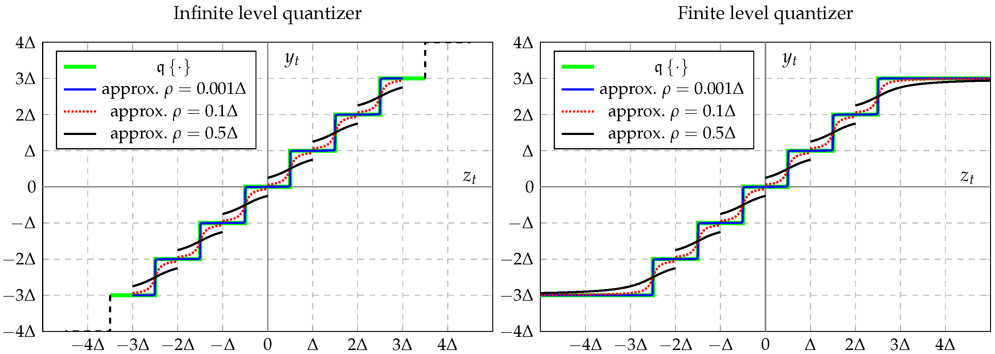
Figure 3.
Quantizer approximation by using the arctan function.
Figure 3.
Quantizer approximation by using the arctan function.
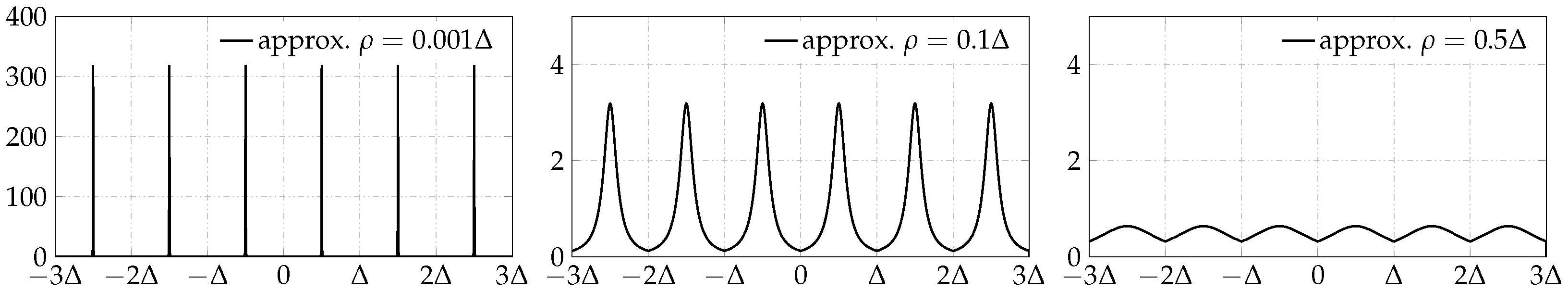
Figure 4.
Jacobian matrix of the quantizer approximation.
Figure 4.
Jacobian matrix of the quantizer approximation.
Figure 5.
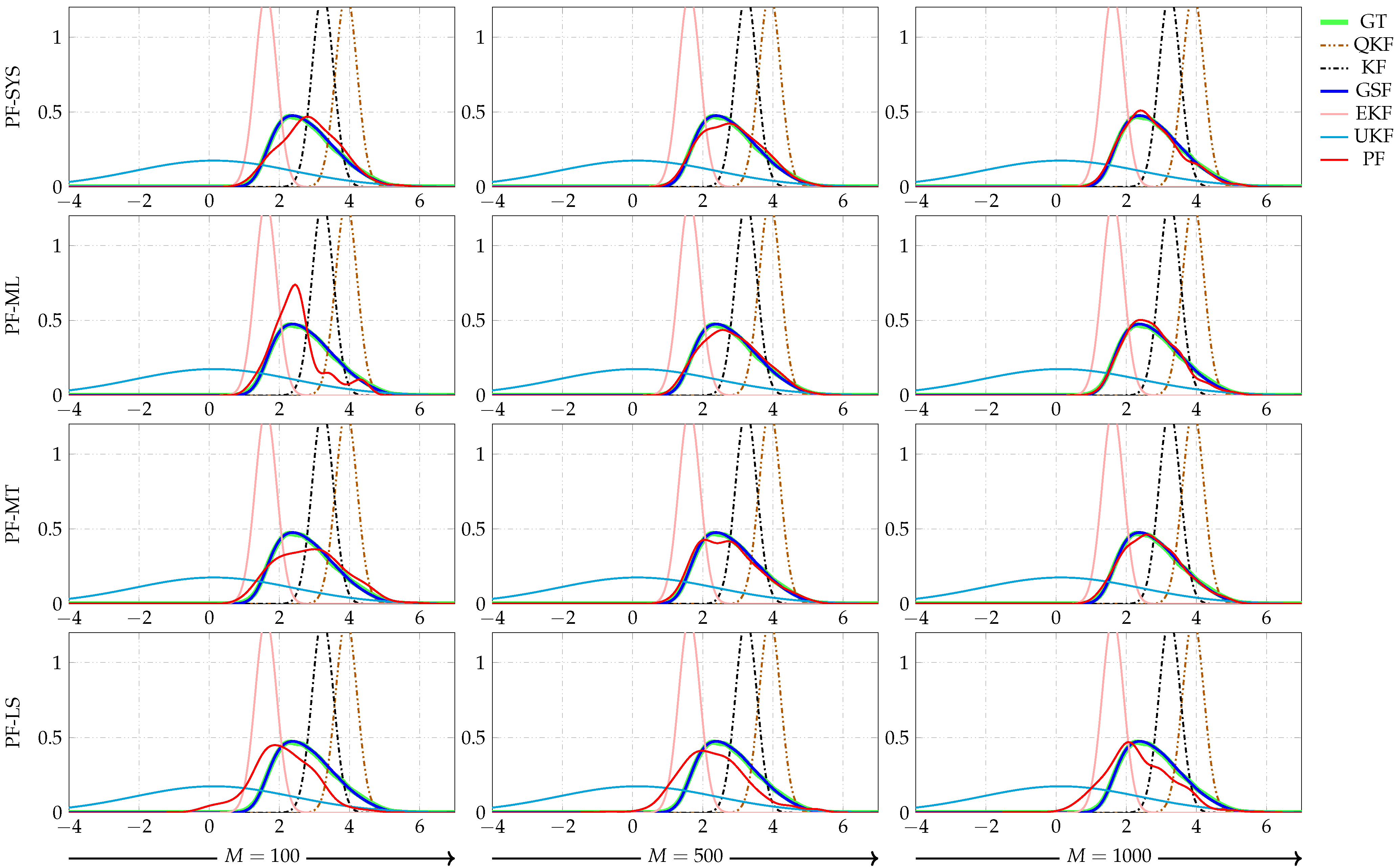
Filtering PDFs for a time instant. GT stands for the ground truth. KF, EKF, QKF, UKF, GSF, and PF stand for Kalman filter, extended Kalman filter, quantized Kalman filter, unscented Kalman filter, Gaussian sum filter, and particle filter, respectively. The PDFs given by the KF, EKF, QKF, UKF were frozen in all plots to observe the behavior of the PF (with RWM moves) when the number of particles increased. SYS, ML, MT, LS stand for systematic, multinomial, metropolis, and local selection resampling algorithms, respectively.
Figure 5.
Filtering PDFs for a time instant. GT stands for the ground truth. KF, EKF, QKF, UKF, GSF, and PF stand for Kalman filter, extended Kalman filter, quantized Kalman filter, unscented Kalman filter, Gaussian sum filter, and particle filter, respectively. The PDFs given by the KF, EKF, QKF, UKF were frozen in all plots to observe the behavior of the PF (with RWM moves) when the number of particles increased. SYS, ML, MT, LS stand for systematic, multinomial, metropolis, and local selection resampling algorithms, respectively.
Figure 6.
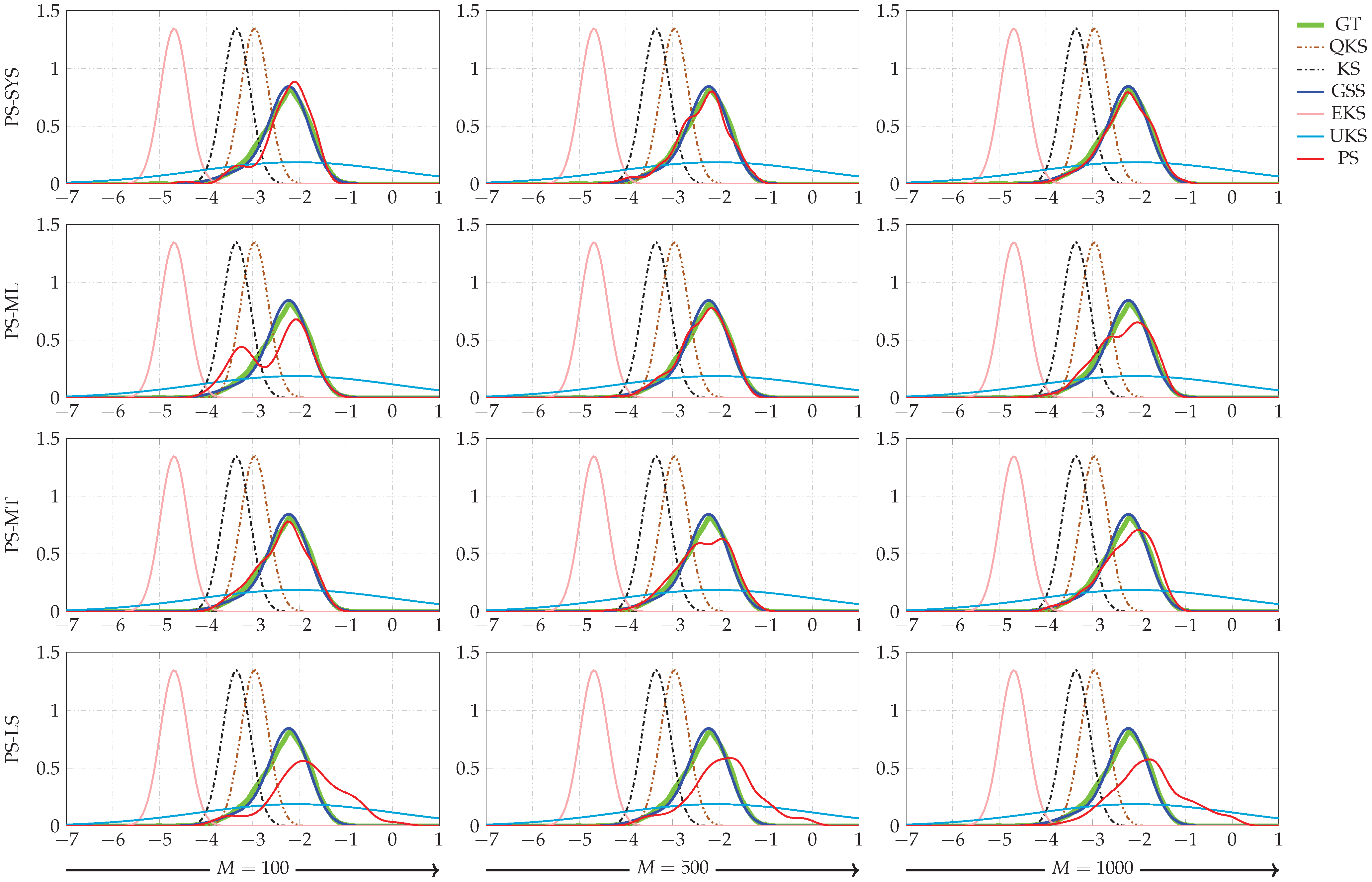
Smoothing PDFs for a time instant. GT stands for the ground truth. KS, EKS, QKS, UKS, GSS, and PS stand for Kalman smoother, extended Kalman smoother, quantized Kalman smoother, unscented Kalman smoother, Gaussian sum smoother, and particle smoother, respectively. The PDFs given by the KS, EKS, QKS, and UKS were frozen in all plots to observe the behavior of the PS (with RWM moves) when the number of particles increased. SYS, ML, MT, LS stand for systematic, multinomial, metropolis, and local selection resampling algorithms, respectively.
Figure 6.
Smoothing PDFs for a time instant. GT stands for the ground truth. KS, EKS, QKS, UKS, GSS, and PS stand for Kalman smoother, extended Kalman smoother, quantized Kalman smoother, unscented Kalman smoother, Gaussian sum smoother, and particle smoother, respectively. The PDFs given by the KS, EKS, QKS, and UKS were frozen in all plots to observe the behavior of the PS (with RWM moves) when the number of particles increased. SYS, ML, MT, LS stand for systematic, multinomial, metropolis, and local selection resampling algorithms, respectively.
Figure 7.
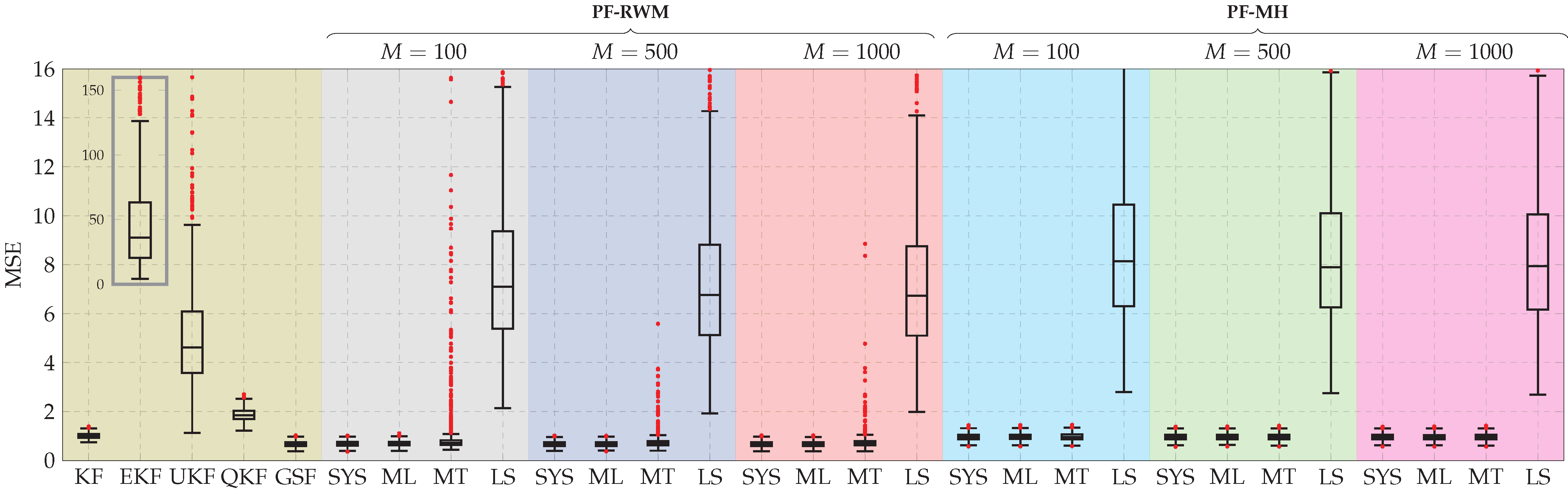
Boxplot of the MSE between the estimated and true state for 1000 Monte Carlo experiments. KF, EKF, QKF, UKF, GSF, and PF stand for Kalman filter, extended Kalman filter, quantized Kalman filter, unscented Kalman filter, Gaussian sum filter, and particle filter, respectively. Additionally, SYS, ML, MT, LS stand for systematic, multinomial, metropolis, and local selection resampling algorithms, respectively. RWM and MH denote random walk Metropolis and Metropolis–Hasting moves.
Figure 7.
Boxplot of the MSE between the estimated and true state for 1000 Monte Carlo experiments. KF, EKF, QKF, UKF, GSF, and PF stand for Kalman filter, extended Kalman filter, quantized Kalman filter, unscented Kalman filter, Gaussian sum filter, and particle filter, respectively. Additionally, SYS, ML, MT, LS stand for systematic, multinomial, metropolis, and local selection resampling algorithms, respectively. RWM and MH denote random walk Metropolis and Metropolis–Hasting moves.
Figure 8.
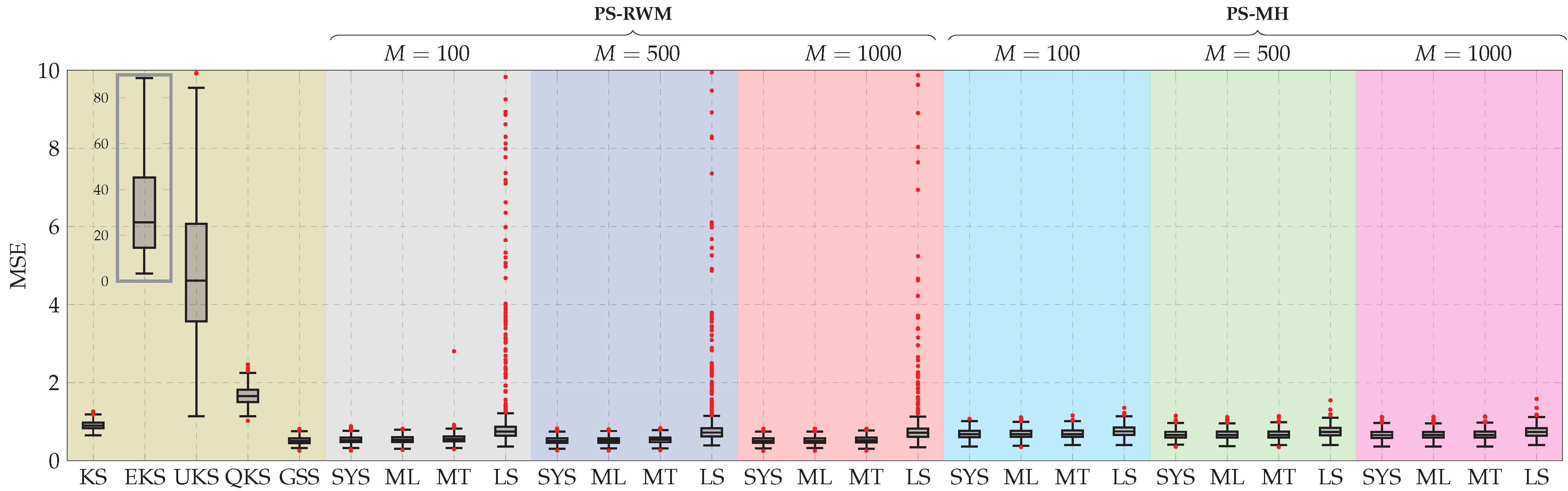
Boxplot of the MSE between the estimated and true state for 1000 Monte Carlo experiments. KS, EKS, QKS, UKS, GSS, and PS stand for Kalman smoother, extended Kalman smoother, quantized Kalman smoother, unscented Kalman smoother, Gaussian sum smoother, and particle smoother, respectively. Additionally, SYS, ML, MT, and LS stand for systematic, multinomial, metropolis, and local selection resampling algorithms, respectively. RWM and MH denote random walk Metropolis and Metropolis–Hasting moves.
Figure 8.
Boxplot of the MSE between the estimated and true state for 1000 Monte Carlo experiments. KS, EKS, QKS, UKS, GSS, and PS stand for Kalman smoother, extended Kalman smoother, quantized Kalman smoother, unscented Kalman smoother, Gaussian sum smoother, and particle smoother, respectively. Additionally, SYS, ML, MT, and LS stand for systematic, multinomial, metropolis, and local selection resampling algorithms, respectively. RWM and MH denote random walk Metropolis and Metropolis–Hasting moves.
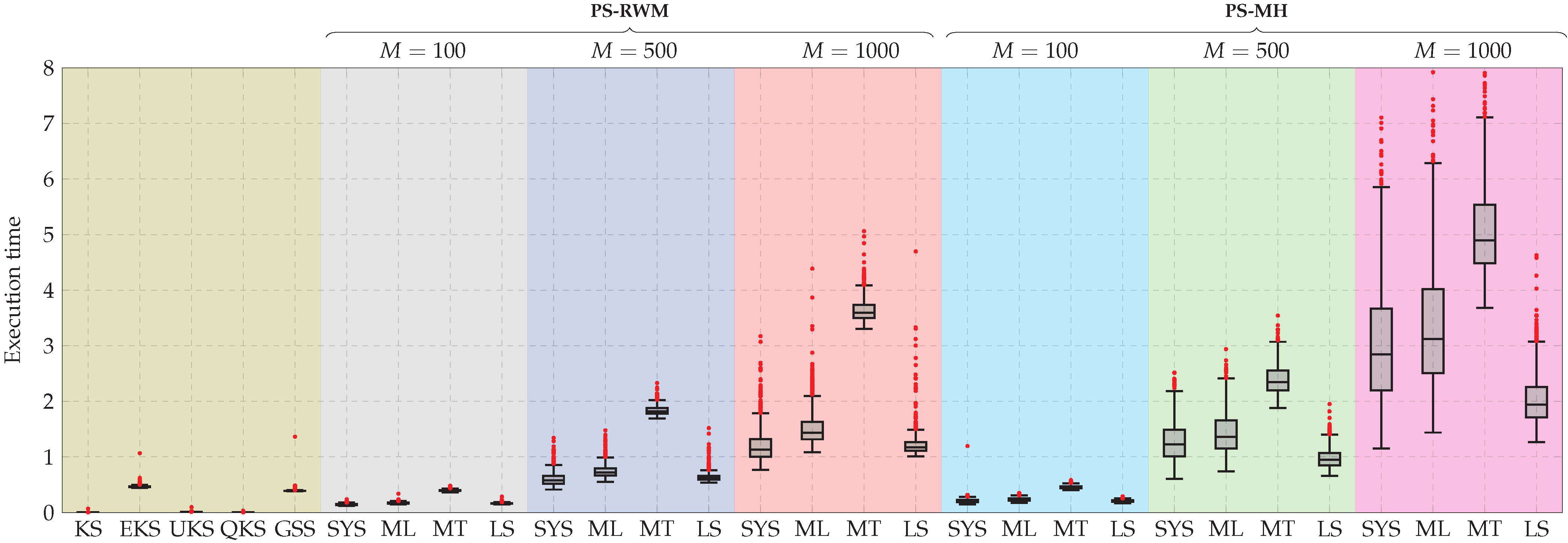
Figure 9.
Boxplot of the execution time for 1000 Monte Carlo experiments. KS, EKS, QKS, UKS, GSS, and PS stand for Kalman smoother, extended Kalman smoother, quantized Kalman smoother, unscented Kalman smoother, Gaussian sum smoother, and particle smoother, respectively. Additionally, SYS, ML, MT, and LS stand for systematic, multinomial, metropolis, and local selection resampling algorithms, respectively. RWM and MH denote random walk Metropolis and Metropolis–Hasting moves.
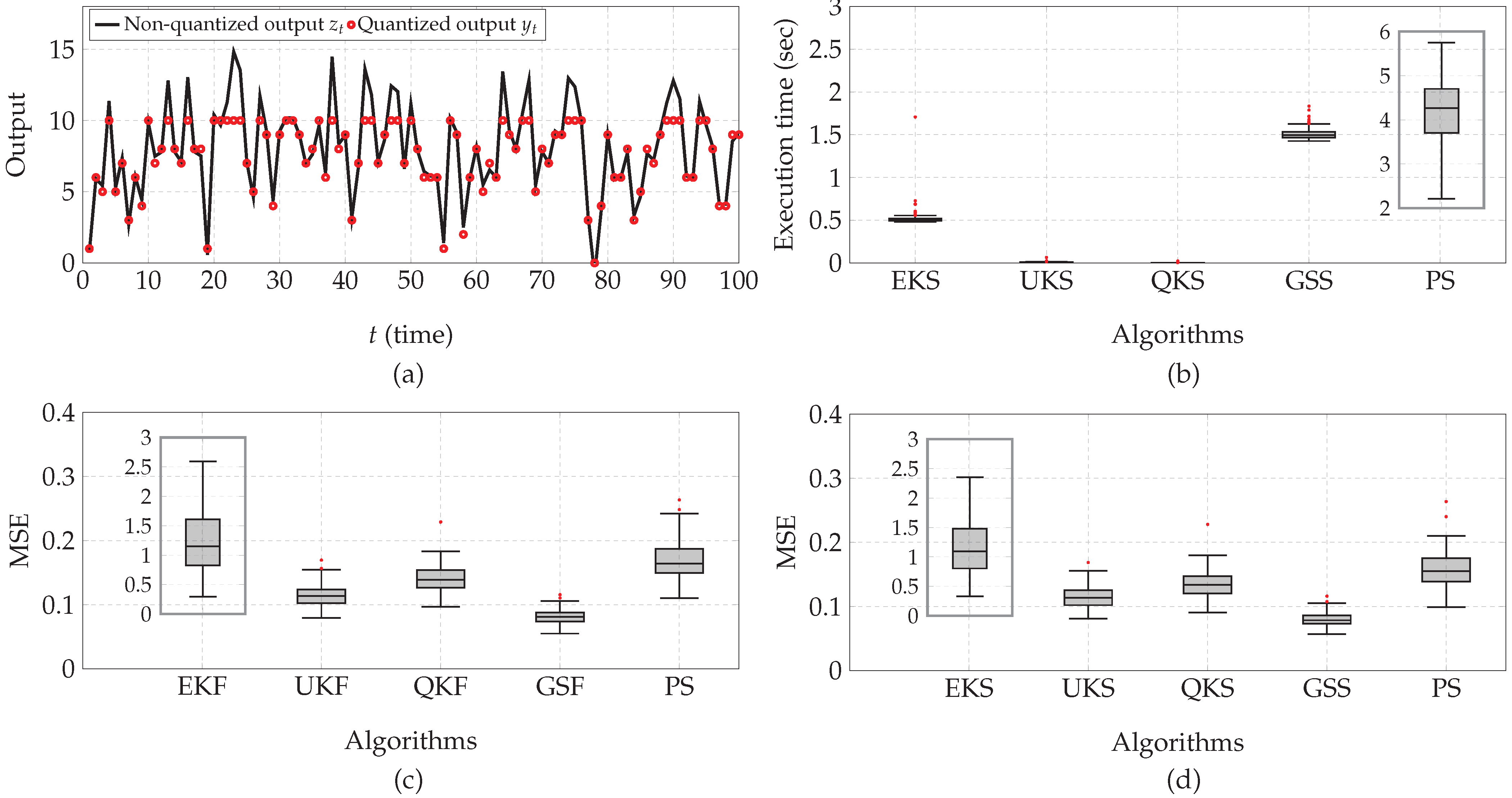
Figure 10.
Practical application: (a) A realization of the non-quantized signal and the quantized output . (b) Boxplot of the execution time of the smoothing algorithms. (c) Boxplot of the MSE between the real and estimated (filtered) tank liquid level. (d) Boxplot of the MSE between the real and estimated (smoothed) tank liquid level. EKF/EKS, QKF/QKS, UKF/UKS, GSF/GSS, and PF/PS stand for extended Kalman filter/smoother, quantized Kalman filter/smoother, unscented Kalman filter/smoother, Gaussian sum filter/smoother, and particle filter/smoother, respectively.
Table 1.
Integral limits of Equation (
17).
Table 1.
Integral limits of Equation (
17).
| FLQ | | | |
| | |
| | |
| | ∞ |
| ILQ | | | |
Table 2.
Parameters of the approximation using the Gauss–Legendre quadrature.
Table 2.
Parameters of the approximation using the Gauss–Legendre quadrature.
| FLQ | | | | |
| | | |
| | | |
| | | |
| ILQ | | | | |
Table 3.
Rank of the filtering and smoothing recursive algorithms for quantized data. References: KF/KS, EKF/EKS [
16], QKF/QKS [
21,
22], PF/PS [
24], UKF/UKS [
16,
18], GSF/GSS [
31,
32]. The notation XX-YY-ZZ(M) denotes the following: XX stands for the filtering or smoothing algorithm (PF or PS), YY stands for the MCMC algorithm (RWM or MH), ZZ stands for the resampling method (SYS, ML, MT or LS), and (M) stands for the number of particles used (100, 500, or 1000).
| Rank | Filtering | Smoothing | Smoothing Execution Time |
|---|
| MSE | Algorithm | MSE | Algorithm | Execution Time | Algorithm |
|---|
| 1 | 0.6724 | GSF | 0.5207 | GSS | 0.0026 | KS |
| 2 | 0.6740 | PF-RWM-SYS (1000) | 0.5212 | PS-RWM-SYS (1000) | 0.0031 | QKS |
| 3 | 0.6744 | PF-RWM-ML (1000) | 0.5220 | PS-RWM-ML (1000) | 0.0111 | UKS |
| 4 | 0.6754 | PF-RWM-SYS (500) | 0.5231 | PS-RWM-SYS (500) | 0.1453 | PS-RWM-SYS (100) |
| 5 | 0.6765 | PF-RWM-ML (500) | 0.5247 | PS-RWM-ML (500) | 0.1644 | PS-RWM-LS (100) |
| 6 | 0.6880 | PF-RWM-SYS (100) | 0.5393 | PS-RWM-MT (1000) | 0.1718 | PS-RWM-ML (100) |
| 7 | 0.6948 | PF-RWM-ML (100) | 0.5415 | PS-RWM-SYS (100) | 0.2077 | PS-MH-LS (100) |
| 8 | 0.7588 | PF-RWM-MT (1000) | 0.5420 | PS-RWM-MT (500) | 0.2109 | PS-MH-SYS (100) |
| 9 | 0.7830 | PF-RWM-MT (500) | 0.5470 | PS-RWM-ML (100) | 0.2354 | PS-MH-ML (100) |
| 10 | 0.9590 | PF-MH-SYS (1000) | 0.5689 | PS-RWM-MT (100) | 0.3931 | GSS |
| 11 | 0.9593 | PF-MH-MT (1000) | 0.6708 | PS-MH-SYS (1000) | 0.3984 | PS-RWM-MT (100) |
| 12 | 0.9595 | PF-MH-ML (1000) | 0.6711 | PS-MH-ML (1000) | 0.4579 | PS-MH-MT (100) |
| 13 | 0.9608 | PF-MH-SYS (500) | 0.6737 | PS-MH-SYS (500) | 0.4676 | EKS |
| 14 | 0.9612 | PF-MH-MT (500) | 0.6746 | PS-MH-ML (500) | 0.6048 | PS-RWM-SYS (500) |
| 15 | 0.9612 | PF-MH-ML (500) | 0.6752 | PS-MH-MT (1000) | 0.6348 | PS-RWM-LS (500) |
| 16 | 0.9686 | PF-MH-SYS (100) | 0.6781 | PS-MH-MT (500) | 0.7469 | PS-RWM-ML (500) |
| 17 | 0.9697 | PF-MH-ML (100) | 0.6927 | PS-MH-SYS (100) | 0.9772 | PS-MH-LS (500) |
| 18 | 0.9715 | PF-MH-MT (100) | 0.6927 | PS-MH-ML (100) | 1.2054 | PS-RWM-SYS (1000) |
| 19 | 1.0138 | KF | 0.6974 | PS-MH-MT (100) | 1.2274 | PS-RWM-LS (1000) |
| 20 | 1.6731 | PF-RWM-MT (100) | 0.7469 | PS-MH-LS (1000) | 1.2709 | PS-MH-SYS (500) |
| 21 | 1.8616 | QKF | 0.7497 | PS-MH-LS (500) | 1.4192 | PS-MH-ML (500) |
| 22 | 5.0549 | UKF | 0.7667 | PS-MH-LS (100) | 1.5197 | PS-RWM-ML (1000) |
| 23 | 7.3381 | PF-RWM-LS (1000) | 0.9100 | KS | 1.8362 | PS-RWM-MT (500) |
| 24 | 7.3602 | PF-RWM-LS (500) | 0.9393 | PS-RWM-LS (1000) | 2.0277 | PS-MH-LS (1000) |
| 25 | 7.6912 | PF-RWM-LS (100) | 1.2900 | PS-RWM-LS (500) | 2.3945 | PS-MH-MT (500) |
| 26 | 8.3846 | PF-MH-LS (1000) | 1.6693 | QKS | 3.0254 | PS-MH-SYS (1000) |
| 27 | 8.4079 | PF-MH-LS (500) | 5.0545 | UKS | 3.3505 | PS-MH-ML (1000) |
| 28 | 8.6717 | PF-MH-LS (100) | 6.4904 | PS-RWM-LS (100) | 3.6364 | PS-RWM-MT (1000) |
| 29 | 47.7827 | EKF | 33.8842 | EKS | 5.0651 | PS-MH-MT (1000) |


 ,
, 


