Action-Based Digital Characterization of a Game Player

Abstract

Games can be more than just a form of entertainment. Game spaces can be used to test different research ideas quickly, simulate real-life environments, develop non-playable characters (game agents) that interact alongside human players and much more. Game agents are becoming increasingly sophisticated as the collaboration between game agents and humans only continues to grow, and there is an increasing need to better understand game players’ workings. Therefore, this work addresses the digital characterization (DC) of various game players based on the game feature values found in a game space, and based on the actions gathered from player interactions with the game space. High-confidence actions are extracted from rules created with association rule mining, utilizing advanced evolutionary algorithms (e.g., differential evolution) on the dataset of feature values. These high-confidence actions are used in the characterization process, resulting in the DC description of each player. The main research agenda of this study is to determine whether DCs manage to capture the essence of players’ action style behavior. Experiments reveal that characterizations do indeed capture behavior nuances, and consequently open up many research possibilities in the domains of player modeling, analyzing the behavior of different players and automatic policy creation, which can possibly be used for utilization in future simulations.

1. Introduction

Games are a great form of entertainment, whether they are board games (e.g., Monopoly™) between friends or an organized video game multiplayer competition with a large pool of rewards available. However, games can also be a significant source of data when studying research questions in various fields (e.g., human–computer interaction) and can therefore act as a reliable scientific tool [1]. One of the important aspects regarding video games is research concerning actions. By examining the actions executed by players during games, researchers can generate innovative theories on player behavior or verify their hypotheses. Such research can also uncover previously unconsidered research topics. An important sub-domain within action research is action abstraction, which attempts to simplify the representation of complex actions into more manageable components (a detailed description of the action abstraction process is provided in the related work section). Such abstracted actions can then be efficiently used by different intelligent algorithms (e.g., machine learning optimization algorithms) in large game spaces.

A game space can be presented as a high-dimensional space of game variants (i.e., adjustable game parameters tune a game toward achieving a desirable player experience, and a unique parameter setting is called a game variant) [2]. When human players begin to interact with virtual game spaces, the game spaces must be fun, because this is what brings enjoyment to the players when they are engaged with the game [3]. To keep the player interested, the need for computer-controlled game players (game agents) begins to form swiftly. However, game agents must offer more than just a random execution of game actions (e.g., imagine a car race where none of the cars stick to the racetrack and just drive around randomly). They must be intelligent.

The computer-controlled game agent is intelligent if it selects actions that help the player to accomplish their goals autonomously [4]. For example, in a game of chess, one way to achieve competition victory is to force an opponent into a checkmate position. The king piece is under attack, or in “check”, if it cannot move to any other position, if it cannot be protected by other game pieces and if the piece that attacked it cannot be taken. In the real-time strategy (RTS) games genre [5], one way to win the game is by eliminating all the opponent’s structures and units.

For several decades, RTS games have offered gamers challenging gameplay and emphasize strategic and tactical decision making. As a result of their demanding gameplay, RTS games have also been used in game research. Players must carefully operate armies of units to gain an advantage over their opponent. The prediction of the opponent’s intentions, tactics and strategies is therefore essential when the game agent must choose which actions can help them achieve their goals in the given game environment, e.g., when predicting the movements of the opponent’s forces to perform appropriate counter-moves [6]. The RTS player must also be skilled in resource management with unit production and deployment; construction of the base; upgrading buildings; being smart about the extensive technology tree, which allows the research of new (or better) units and technologies; and sometimes even being versed in diplomacy. Split-second decisions and fast-paced real-time gameplay also heavily characterize RTS games.

Data mining is an interdisciplinary field inspired by the principles of other scientific areas, such as mathematics, statistics and physics. It is primarily intended for discovering hidden information in data. Data mining encompasses several methods, and association rule mining (ARM) is one of them, which is a well-known technique intended for identifying the relationships between attributes in transaction databases. Loosely speaking, association rules reveal information between items (e.g., “chocolate is followed by banana,” meaning customers who buy chocolate also buy bananas). The first applications of ARM were tailored to the applications of market basket analysis, where association rules helped in the decision process of, for example, how to place products on supermarket shelves. Later, ARM began to be used in many applications, ranging from medicine to data science and engineering.

To predict an opponent’s intentions, we previously proposed a method for opponent game policy modeling using ARM (ogpmARM) [7]. In this work, the formerly built method was extended with additional components, and the result was a new method called digital characterization with ARM (dcARM). The dcARM method was adapted to allow for a range of purposes besides only opponent modeling, such as for game agents’ digital characterization (DC) (i.e., an action-based digital representation of the game player). Generally speaking, the DC captures the essence of the players by reflecting their action styles, behaviors and playing preferences. Specifically, DC, from a technical point of view, represents an action pattern of the whole player action behavior for a given game time interval (e.g., the last one hundred frames) with a set frame step (e.g., the resolution of every five frames).

The contributions of this paper regarding the dcARM method are as follows:

(a)

To test the method in two experiments of various complexities. The first is a case study on the simple (yet powerful) game of Rock–Paper–Scissors (RPS). RPS is a game typically played between two players, in which each player simultaneously chooses one of three actions: rock, paper or scissors. A set of rules determines the winner: rock beats scissors, scissors beat paper and paper beats rock (such game relationships between rock, paper and scissors can also be found in several natural systems [8]). The second experiment is carried out in the complex environment of RTS games.

(b)

To perform a DC analysis and a time analysis on the DCs created using the feature and action data of five game agents while they operate in a complex RTS game environment.

(c)

To establish the DC method’s suitability for real-time (online/in-game) usage capabilities.

(d)

To discuss its possible usage in automated policy creations, in future simulation purposes or with a DC serving as a vital part in the game agent’s decision-making process.

Some of the novelties presented in this article are as follows:

(a)

To our knowledge, this is the first approach for using association rule mining in a game domain where the mined rules are not used in their entirety (e.g., for building a game knowledge database), but only as guiding factors (by utilizing rules thresholds in descending order), allowing for the discovery and extraction of actions with a higher confidence value, and, consequently, using that information for building quality abstracted player action representations.

(b)

The method creates explainable (interpretable) player action representations (e.g., deep-learning-based agents/models are hard to interpret [9], but this method’s action representations can be interpreted more easily).

(c)

The approach confirms that the output of the dcARM method shows differences in game agent action usages (i.e., which actions are used more and which are used less).

(d)

By comparing the differences in how agents are using actions, the (sub)patterns of comparable behavior can be established between different agents.

The structure of this article is as follows. The related work belonging to a game domain connected to this research is presented in the Section 2. Section 3 presents the materials and methods. In Section 4, a case study of the game environment of the RPS game proves the dcARM’s ability to create reliable DCs. Section 5 follows, with an experiment in an RTS simulation environment, and Section 6 provides a discussion covering all the findings of the Section 5 experiment. The article concludes with final remarks in Section 7.

2. Related Work

This section reviews the related work concerning game actions in real-time environments, focusing on creating models, patterns and policies.

To play a game, the game agent needs to have at least an observable game state and a set of available actions [10]. Most games assume the existence of some model of the game that allows one to evaluate a current game state and to predict a new game state after executing a certain action [11,12]. To predict the next meaningful sequence of actions that would contribute toward the ultimate game agent goals, the game agents utilize various techniques (e.g., a decision tree search). The number of units that can make actions in each turn is also large, and the game agent needs to handle them all simultaneously. However, an exhaustive evaluation of every possible action for each unit in the game space is not feasible due to the vast number of combinations. For example, in StarCraft™, this number can reach between 30⁵⁰ and 30²⁰⁰ [13].

Furthermore, deciding which actions would be the most beneficial is not straightforward. The agent must usually peruse the long-term rewards with a sequence of actions (e.g., with reinforcement learning techniques [14]). Consequently, specific patterns emerge from action sequences. These patterns can be used for simplification. Instead of generating specific commands one by one, the game agent can apply a sequence of actions corresponding to different patterns.

The RTS game genre used in this article is an example of games operating under strict real-time constraints [15]. In casual chess gameplay, whether the player makes a move in one or five minutes is irrelevant for gameplay. RTS games operate in dedicated time slices. A time slice is allocated between two game frames during which a game agent can perform some actions. The duration of the time slice is usually less than 100 [16] and around 30 [17] or 42 [18] milliseconds. If that time slice is missed, the game iterates to the next game frame, where the game agent is eventually given another opportunity to decide which actions should be executed.

Some simplification is required to cope with the complexity and severe timing constraints of RTS games. The most common simplification is the hierarchy abstraction [13]. The decision processes are usually divided into three layers: reaction control, tactics and strategy. The reaction control layer is responsible for micromanaging the units, the tactic layer deals with groups of related units, and the strategic layer is responsible for achieving the game’s ultimate objective. The dedicated game agent sub-component is allocated for each layer. Depending on the game scenario, these layers can be further divided horizontally or vertically.

Next are the game model and action abstractions [19,20]. The first reduces the game-state complexity by reducing the level of detail, and the second generalizes the gameplay actions. The reaction control layer requires a detailed description of the game state, focused only on the location of the specific unit and its surroundings in the game world. It operates with game actions and changes the game state. The tactical layer works on the broader area with fewer details (e.g., with the estimated attack power or defense strength of a group of units). The actions work on the grouping of units and must be translated into the specific game actions by the reaction control layer. The strategic layer is responsible for the general policy of the gameplay. It makes decisions regarding goals, roles and relations between the unit groups. For example, the rushing policy focuses all resources on storming the opponent at the start of the game. Of course, the strategic layer also tries to detect the opponent’s policy to counteract its actions properly. All the abstractions reduce the processing time of the game agent to work in real time significantly [21].

The game agent can split its computations between the frames and choose if and at what time it will execute specific actions on each layer. The estimated time intervals for each hierarchical layer are [22] up to one second for the reaction control layer, thirty to sixty seconds for the tactical layer and three minutes or more for the strategic layer.

3. Materials and Methods

This section first establishes how the game agents utilize different types of knowledge acquisition and categorizes the dcARM method according to the knowledge acquisition category. Then, descriptions of the feature and action are presented, which are crucial method inputs when combined in a record set. Second, ARM is explained, which is a fundamental component of the method. Third, the software built by the usage of ARM is depicted. Fourth, ARM-DE (differential evolution) algorithm descriptions are provided. Last, the dcARM method pseudocode and the structure of digital characterization with the dcARM method are introduced.

3.1. Game Knowledge Acquisition

Game agents can acquire knowledge in several ways, for example, by interacting with the environment and extracting information from it (automatic approach), with beforehand provision of the knowledge (i.e., a hand-made expert knowledge approach) or by utilizing both techniques [23]. The entirely hand-made expert knowledge incorporation can be intractable for many games (i.e., the game spaces are too dynamic, vast and hard to predict), as well as consuming both energy and time [24]. Both techniques are used in our previous work on the ogpmARM method. For the dcARM method, the expert knowledge approach is only kept in the first step of the method, where features and actions are defined, and the other steps are automatic.

The feature is a low-dimensional representation of the original data [25], where, in the case of the game domain, it can be said that the original information is represented in the form of the full game state (i.e., physical and abstract representation of the map, the state of all players, the positions and states of all units on the map, etc.). Only the features relevant to the game space that the player is in are selected in the case of the dcARM method. The process of hand feature selection is inspired by similar work, such as [26] (e.g., the number of each unit type and gathered resources). In future work, the focus will also be on automatizing the feature selection step.

The player plays the game through the execution of an action, or, depending on the game, through many actions. These actions are combined with feature values extracted from the game state and are saved in a record set. The record set can be seen as a history of a game played so far by the player, or (some sort of) as a replay that usually encodes expert domain knowledge of the gameplay [26], because it holds the information as well as all the actions that the player performed. It must be stated that, because only some of the information value is saved from the game state (via feature abstractions), the replay does not allow for a complete recreation of the gameplay but still encapsulates its essence.

3.2. Stochastic Population-Based Nature-Inspired Algorithms for Association Rule Mining

In this subsection, first, the descriptions are made regarding the stochastic population-based nature-inspired algorithms, numeric association rule mining and uARMSolver software. The action extraction procedure and action intensity pattern are established second.

3.2.1. Stochastic Population-Based Nature-Inspired Algorithms

The term stochastic population-based nature-inspired algorithms depicts the search algorithms inspired mainly by the behavior of natural and biological systems. These algorithms are intended to solve complex optimization problems in both continuous and discrete domains. Evolutionary and swarm intelligence algorithms are the most common members of this group of algorithms. Both groups consist of individuals that have undergone several variation operators (e.g., crossover and mutation) and form a new population. One of the most state-of-the-art algorithms in current use is differential evolution (DE), an evolutionary algorithm in which individuals are represented as vectors consisting of floating-point values. DE is a compelling method for optimization that achieves robust results when dealing with optimization problems in continuous yet discrete domains. DE is also notable for having a low number of control parameters. Besides the population size parameter, DE has two parameters: F and CR. F is a scaling factor, and CR is the crossover rate [27]. Several variants based on DE have also won many CEC competitions for numerical optimization.

3.2.2. Numeric Association Rule Mining (NARM)

ARM is a technique proposed initially for market basket analysis to search for relationships between attributes in a database [28,29,30]. The association rules consist of two parts, representing relationships between attributes: the left part is the antecedent, and the right is a consequent. The quality of the association rules is evaluated using quality measures. The most common are support and confidence, but lift, coverage and amplitude are also widely used measures. Readers are invited to consult [31] for more information about quality measures. The first ARM approaches were only able to deal with categorical data, but later, more enhanced methods appeared that were also able to work with attributes in the continuous domain. These approaches are usually called numerical association rule mining (NARM) [31].

Due to the complexity of such problems, meaning dealing with continuous and discrete attributes, most of the enhanced methods were built on stochastic population-based nature-inspired algorithms, because they can search in a vast search space.

3.2.3. uARMSolver Software

uARMSolver [32] is an open-source implementation of algorithms for dealing with NARM. uARMSolver is written entirely in C++ and allows fast searching for association rules. The abovementioned DE algorithm is included as a base algorithm and is modified to deal with NARM problems. The significant advantage of uARMSolver is that the software covers almost all ARM steps—preprocessing, mining and visualization—which is also partly supported by the current version of this software.

3.2.4. ARM-DE (Differential Evolution) Algorithm

uARMSolver is fundamentally based on the ARM-DE algorithm, in which each individual in the evolutionary algorithm is represented as a real valued vector covering numerical and categorical attributes.

The numerical attribute is represented in this vector by corresponding minimum and maximum boundaries determining domain values from which the attribute can be drawn. On the other hand, the categorical attribute is represented by the real value drawn from the interval [0, 1] [33]. The fitness function is modeled as a weighted sum of support and confidence evaluation metrics. In ARM-DE, the optimization process is governed by DE, but uARMSolver can operate with any other population-based metaheuristic algorithm.

3.2.5. Action Extraction Procedure and Action Intensity Pattern

Action extraction from the ARM rules is a straightforward procedure:

• ARM creates the ruleset based on the feature and action dataset provided to it. If the player makes multiple actions for a given frame, the features of that game frame are duplicated, with only the actions being differing factors between such records. The dataset for ARM includes all the records for a period of maximum passed time t_mpt.
• A set of actions are defined, which are extracted from the ruleset, the action counter set and the threshold at which searching for actions is stopped.
• The ruleset is traversed rule by rule in a threshold-descending manner (i.e., from rules with the highest threshold downward toward the rules with the lowest threshold) until the stopping threshold is met.
• Each rule is parsed and searched for the inclusion of any actions from the set of actions.
• The counter for that specific action is increased if any action from the set of actions is found in the rule.

To the extracted action counter set, the additional abstracted information, such as percentage distributions and the most represented action(s) of the set (action(s) with maximum value(s)), can be added (with other extensions of abstracted information also being possible). The action set with additionally abstracted information added is called the action intensity pattern (AIP) and is shown in Figure 1.

An example of one such AIP would be as follows:

• Frame number: 20 (e.g., included frames are in the interval [1, 20]).
• Extracted actions: 1, 1, 0, 0, 5, 1.
• Percentage distributions of extracted actions: 12.5%, 12.5%, 0%, 0%, 62.5%, 12.5%.
• Maximum action (62.5%): 4.

3.3. dcARM Method and the Game P layer’s Digital Characterization

Algorithm 1 is the pseudocode of the dcARM method.

The first step of the pseudocode defines the manually chosen features and actions, the rule confidence threshold θcv, the maximum passed time for keeping records t_mpt, the maximum passed time for keeping an AIP t_AIP and the sampling rate (e.g., periodically every 20 frames). The feature values are saved in the record set in the second step. In step three, ARM is run with the record set. Steps four and five are modified extensively for the dcARM method. In the previous ogpmARM method, the fourth step was used to match the extracted actions from rules to the predefined policies, but in the dcARM method, an AIP is now created instead. AIPs are the main elements for updating the DC of a player.

Algorithm 1: Pseudocode of the dcARM method

// Step 1—Define input arguments Input: names (set of names of relevant game state features and a player executed actions), θcv (rule confidence value threshold), tmpt (maximum passed time for keeping records), tAIP (maximum passed time for keeping an AIP), sampRat (sampling rate) Output: Digital Characterization (DC) of a player/game agent

set digChar = initializeEmpty() // init. digital characterization currentFrame = 0 do  if currentFrame mod sampRat equals 0 then   // Step 2—Save the feature values in the record set   set playerAction = getPlayerAction(playerID, gameState)   set featureValues = getFeatureValues(playerID, gameState, names)   recordSet = addToRecordSet(recordSet, listOfActions(playerAction), featureValues)   recordSet = removeRecordsOverTimeLimit(tmpt)   // Step 3—Execute ARM and extract actions from rules   setOfActions = extractActions(executeARM(recordSet), θcv)   // Step 4—Create action intensity pattern   AIP = createActIntPat(setOfActions)   // Step 5—Digital characterization of a game agent   digChar = removeOldActIntPatOverTimeLimit(playerID, tAIP)   digChar = updateDigitalCharOfAgent(playerID, AIP)  end if   // DC can be used for automated game policy creations   // DC can be used in future simulations   // DC as the driver of Game Agents’ decision process   // DC can be used for opponent modeling   // … while gameInProgress(gameState)

The structure of the DC can be observed in Figure 2.

4. Case Study: Rock–Paper–Scissors Game

The RPS game is a simple hand game in which two players compete for victory and defeat using three different hand signs (rock, paper or scissors) [34]. The rules of the game are straightforward. Rock wins over scissors (“the rock breaks the scissors”), scissors win over paper (“the scissors cut the paper”), and paper wins over rock (“the paper covers the rock”). It is easily observed that these three rules, each consisting of two actions with different dominances, form a cycle. In other words, due to the present spatial and temporal behaviors that allow for an understanding of properties in various cyclic systems, the RPS game is also known as one of the simplest cyclic dominance models [35].

The reason for selecting this game as a case is due to three factors:

(a)

The simplicity of incorporating only three non-durative and instant actions/hands.

(b)

The possibility of inferring the other player’s strategy and its win rate [36].

(c)

The RPS cyclic game rule principles can be scaled to higher complexities (e.g., the Rock–Scissors–Paper–Lizard–Spock game [37]) and can incorporate different game mechanics/abstractions (e.g., the RPS system as an RTS game cyclic strategy selection [38]), which opens up possibilities for research in many more (game) (sub)domains.

Due to the possibility of inferring the player’s win rate in RPS, the dcARM method is tested on two player strategies: a strategy incorporating non-biased random action taking, and a strategy with biased random action taking.

In summary, using two different strategies, determining whether a successful distinguishment between the non-biased and biased action taking with dcARM is possible (i.e., testing whether the AIPs indicate the bias when the biased action is being used).

4.1. Experimental Settings

Hardware: The case study is carried out on an Intel(R) Core(TM) i7-9700 CPU @ 3.00 GHz, with eight cores and 32 GB RAM. Software: IntelliJ IDEA 2021.1.1 tools with JDK 13.0.2 on an OS Win 10 Pro are utilized in the experiment. uARMSolver uses the (default) following values: algorithm = DE, DE_NP = 100 (population size), DE_FES = 1000 (number of function evaluations), DE_RUNS = 1 (number of DE runs), DE_F = 0.5 (scaling factor), DE_CR = 0.9 (crossover rate) and DE_STRATEGY = 6 (identifier of the DE strategy implemented in uARMSolver).

In the case study experiment, for the first strategy scenario, both players execute actions at random. In contrast, in the second strategy, the first player has a fixed bias toward using a pre-set action (i.e., for the fixed percentage of the number of games, it picks the pre-set action). In the other cases, any of the three actions are chosen at random. The game is run in blocks, in which each block represents fifty thousand games (50 K), reflected in 50 K feature value records saved in the record set. One feature value record is formatted as follows: the number of rocks (chosen by players), the number of papers, the number of scissors and the action that the first player played. Each block is executed 100 times for two reasons/benefits: first, multiple executions of each block must be carried out for the results of an experiment to be representative (i.e., the game is stochastic due to the usage of random action taking), and second, the value 100 coincides with the percentage logic, making the results easier to interpret (e.g., if, in the 33 blocks, the maximum number of times that the action taken is rock, it can be easier to infer that the distribution of rocks during the experiment run is 33 percent). The dcARM method is executed on the record set of only one player for every single block of games.

4.2. Results of the Case Study Experiment

The results of the case study experiment are presented in

Table 1. Summary (across all blocks) of how often each action achieves the maximum action count in rules per block.

	0.1	0.2	0.3	0.4	0.5	0.6	0.7	0.8	0.9	1.0
0%	0/1/28/38/33	0/2/29/38/31	0/4/27/37/32	0/2/30/32/36	0/2/29/35/34	0/6/31/35/28	0/13/36/23/28	E: 100	E: 100	E: 100
10%	0/4/39/27/30	0/1/40/31/28	0/2/35/34/29	0/5/50/29/16	0/2/63/19/16	0/5/51/25/19	0/1/96/1/2	43/0/57/0/0	E: 100	E: 100
20%	0/3/43/25/29	0/2/46/27/25	0/2/42/24/32	0/11/52/19/18	0/3/73/17/7	0/4/78/8/10	0/2/98/0/0	0/0/100/0/0	E: 100	E: 100
30%	0/4/74/8/14	0/1/81/7/11	0/1/86/6/7	0/2/89/4/5	0/0/99/0/1	0/0/100/0/0	0/0/100/0/0	0/0/100/0/0	E: 100	E: 100
40%	0/2/84/6/8	0/4/86/4/6	0/2/85/7/6	0/1/97/1/1	0/0/100/0/0	0/0/99/1/0	0/0/100/0/0	0/0/100/0/0	E: 100	E: 100
50%	0/1/89/7/3	0/1/89/5/5	0/1/89/2/8	0/0/99/1/0	0/0/100/0/0	0/0/100/0/0	0/0/100/0/0	0/0/100/0/0	E: 100	E: 100
60%	0/0/93/5/2	0/2/84/6/8	0/2/96/2/0	0/0/100/0/0	0/0/99/0/1	0/0/100/0/0	0/0/100/0/0	0/0/100/0/0	0/0/100/0/0	E: 100
70%	0/0/100/0/0	0/0/100/0/0	0/0/100/0/0	0/0/100/0/0	0/0/100/0/0	0/0/100/0/0	0/0/100/0/0	0/0/100/0/0	0/0/100/0/0	E: 100
80%	0/0/100/0/0	0/0/100/0/0	0/0/100/0/0	0/0/100/0/0	0/0/100/0/0	0/0/100/0/0	0/0/100/0/0	0/0/100/0/0	0/0/100/0/0	E: 100
90%	0/0/100/0/0	0/0/100/0/0	0/0/100/0/0	0/0/100/0/0	0/0/100/0/0	0/0/100/0/0	0/0/100/0/0	0/0/100/0/0	0/0/100/0/0	E: 100
100%	0/0/100/0/0	0/0/100/0/0	0/0/100/0/0	0/0/100/0/0	0/0/100/0/0	0/0/100/0/0	0/0/100/0/0	0/0/100/0/0	0/0/100/0/0	0/0/100/0/0

and

Table 2. Averaged (across all blocks) percentage distributions of counted actions per block.

	0.1	0.2	0.3	0.4	0.5	0.6	0.7	0.8	0.9	1.0
0%	31.71/33.56/34.73	33.28/34.35/32.37	33.48/32.68/33.84	33.51/32.38/34.11	32.33/34.66/33.01	32.9/33.97/33.13	35.87/30.59/33.54	0/0/0	0/0/0	0/0/0
10%	36.14/32/31.86	35.71/32.5/31.79	35.77/32.16/32.07	38.44/32.4/29.16	40.66/29.31/30.03	40.02/30.31/29.67	59.96/19.28/20.76	100/0/0	0/0/0	0/0/0
20%	37.36/30.64/32	37.66/31.23/31.11	37.03/31.28/31.69	39.05/31.86/29.09	43.09/30.41/26.5	43.69/29.42/26.89	60.74/19.87/19.39	100/0/0	0/0/0	0/0/0
30%	43.44/27.98/28.58	44.34/27.1/28.56	44.87/27.25/27.88	47.07/27.11/25.82	57.27/20.92/21.81	60.83/19.84/19.33	73.79/13.14/13.07	100/0/0	0/0/0	0/0/0
40%	45.09/26.37/28.54	45.66/27.15/27.19	46.7/27.07/26.23	54.46/23.48/22.06	58.15/21.44/20.41	61.44/19.45/19.11	78.33/10.72/10.95	100/0/0	0/0/0	0/0/0
50%	47.24/25.75/27.01	47.29/27.77/24.94	47.95/25.19/26.86	56.46/20.44/23.1	58.9/21.11/19.99	64.93/17.13/17.94	80.14/9.8/10.06	100/0/0	0/0/0	0/0/0
60%	48.02/27.03/24.95	47.55/26/26.45	52.18/23.16/24.66	58.38/20.9/20.72	59.88/20.11/20.01	66.64/16.94/16.42	84.38/7.71/7.91	100/0/0	100/0/0	0/0/0
70%	65.24/17.51/17.25	65.46/16.95/17.58	68.48/15.7/15.82	74.88/11.81/13.31	76.49/11.66/11.85	80.35/9.92/9.73	96.39/1.82/1.79	100/0/0	100/0/0	0/0/0
80%	64.77/17.19/18.04	64.99/17.85/17.16	74.48/12.93/12.59	76.3/11.38/12.32	76.96/11.41/11.63	79.93/9.72/10.35	100/0/0	100/0/0	100/0/0	0/0/0
90%	69.55/15.21/15.24	73.64/13.37/12.99	78.94/11.11/9.95	80.25/9.41/10.34	80.78/9.35/9.87	94.15/2.92/2.93	100/0/0	100/0/0	100/0/0	0/0/0
100%	100/0/0	100/0/0	100/0/0	100/0/0	100/0/0	100/0/0	100/0/0	100/0/0	100/0/0	100/0/0

. Table 1 shows the summary (across all blocks) of how many times each action achieved the maximum action count in rules per block. Table 2 presents the averaged (across all blocks) percentage distributions of counted actions per block. The data regarding the averages (across all blocks) of the counted actions per block are also included in Appendix A in

Table A1. Averages (across all blocks) of the counted actions per block.

	0.1	0.2	0.3	0.4	0.5	0.6	0.7	0.8	0.9	1.0
0%	32.58/34.53/36.01	33.96/35.09/33.16	34.74/34.28/35.19	31.54/30.68/32.05	23.75/25.47/24.47	20.95/21.57/21.06	7.2/6.1/6.61	0/0/0	0/0/0	0/0/0
10%	36.98/32.7/32.35	37.83/34/33.66	36.41/32.65/32.38	36.64/30.57/27.74	32.15/23.49/23.75	25.02/18.53/18.26	19.14/6.01/6.51	8.12/0/0	0/0/0	0/0/0
20%	38.76/31.7/33.04	39.42/32.68/32.54	38.81/32.76/33.06	37.89/30.97/27.98	34.28/24.14/21.19	25.98/17.23/15.95	19.28/6.2/6.06	8.44/0/0	0/0/0	0/0/0
30%	48.34/30.94/31.36	49.4/30.16/31.45	50.39/30.19/31.13	49.37/27.98/26.8	50.26/18.21/19	47.26/15.15/14.62	30.91/5.41/5.32	17.25/0/0	0/0/0	0/0/0
40%	50.24/29.02/31.56	50.63/29.87/29.65	51.19/29.59/28.83	50.97/21.66/20.35	50.98/18.64/17.86	47.32/14.76/14.52	37.22/4.97/5.09	16.38/0/0	0/0/0	0/0/0
50%	53.42/28.87/30.12	54.01/31.49/28.3	49.86/25.69/27.43	53.29/18.94/21.49	52.59/18.77/17.56	53.31/13.79/14.56	40.52/4.82/4.95	30.67/0/0	0/0/0	0/0/0
60%	53.86/30.01/27.66	52.52/27.99/28.88	54.63/23.96/25.51	54.77/19.21/19.09	50.73/16.87/16.77	53.11/13.33/12.84	46.51/4.11/4.27	34.29/0/0	17.13/0/0	0/0/0
70%	106.94/28.34/27.69	107.9/27.48/28.65	108.31/24.48/24.35	106.37/16.53/18.69	106.28/15.93/16.27	104.49/12.63/12.56	104.7/1.93/1.98	87.57/0/0	53.25/0/0	0/0/0
80%	106.43/27.84/29.1	107.84/29.22/28.05	107.32/18.44/17.93	105.22/15.42/16.53	105.39/15.36/15.83	106.94/12.84/13.51	106.48/0/0	94.65/0/0	65.53/0/0	0/0/0
90%	131.04/28.18/28.13	136.65/24.62/23.79	137.01/19.01/16.97	135.25/15.79/17.21	134.03/15.22/16.06	133.65/4.09/4.11	138.37/0/0	127.01/0/0	90.38/0/0	0/0/0
100%	164.75/0/0	165.34/0/0	164.55/0/0	165.13/0/0	163.65/0/0	166.71/0/0	165.39/0/0	165.06/0/0	146.01/0/0	88.1/0/0

.

The tables range from 0 to 100 percent bias toward a specific action and from a 0.1 to 1.0 rule confidence value threshold. The rule confidence value of 0.0 is omitted from the tables, because a rule with a confidence value of 0.0 is a non-meaningful rule (i.e., it provides no trust). The first line of each table shows the results of the first strategy (no action bias present), and the rest of the table results belong to the second strategy (biased action). For the case study, the rock action is chosen to represent a biased action. In the case of selecting two other actions as biased, the results should be very similar due to the equality of actions (i.e., their strength is the same).

Each cell in Table 1 holds five values. The first value represents the number of times actions came up empty (E) (i.e., if no actions are found in the rules equal to or above the rule confidence value threshold). The second value represents the number of times that at least two actions achieve the same maximum value (i.e., when two or three actions achieve the same action count from the set of rules of a single block). The third value is the number of times that only rock has the maximum value, the fourth is the number of times that only paper has the maximum value, and the fifth is the number of times that only scissors have the maximum value.

Table 2 shows the calculated average percentage distributions. The percentage distributions are calculated for all three blocks’ actions. The average of the percentage distributions is calculated for all blocks except for the blocks marked as (E); these are omitted from the average calculations to maintain the focus of the case study on action percentages alone (i.e., all the percentages of actions sum to one hundred, which allows for a more transparent presentation of the results). (E)s are, for the same purpose, also omitted from Table A1. In Table 2 and Table A1, the values in each cell represent the measured values for RPS actions in the following order: rock, paper and scissors (e.g., the measured values 100/0/0 in Table 2 show that the rock action has a 100 percent average distribution (across all blocks) of the counted actions per block).

4.3. Short Discussion of the Results of the Case Study Experiment

The gathered data presented in Table 1, Table 2 and Table A1 show that the biased rock action values are higher than the values of the other two non-biased actions as soon as the biased percentage increases above 0 percent. For example, in Table 1, the 10 percent biased rock action values for a threshold of 0.7 are 96 (out of 100), the value in Table 2 is 59.96 percent, and the other two actions receive 19.28 and 20.76 percent. This is a clear indicator of the method’s capability to create viable AIPs, because the data reveal even a 10 percent increase in the bias of specific actions.

It is also clear that the threshold value parameter is vital in choosing the AIP into which a high degree of confidence is entrusted. For example, from the results from Table 1, if the 0 percent and 0.7 threshold values (0/13/36/23/28) and the 10 percent and 0.1 threshold values (0/4/39/27/30) are compared, they are very similar. This means that, if the information regarding which data are linked to 0 percent and which are linked to 10 percent is not also provided, a high degree of confidence distinguishment between both results is not possible. However, when comparing the 0 percent record (0/13/36/23/28) with the 10 percent record (0/1/96/1/2) for a threshold of 0.7, the difference between both rock action values (36 for 0 percent and 96 for 10 percent) is noticeable.

When observing the data in Table 1, the thresholds of 0.7 and 0.8 stand out as the best options, because the recorded values for the rock action are 100 or very close to this number, whereas for the other two actions, they are zero or very close to it. However, when the data from Table 2 are also taken into account, the threshold of 0.8 is the apparent winner, because, for this threshold, a 100 percent confidence in the rock action is shown across all the biased percentage values. The data in Table 2 indicate that percentage distributions may be a better choice for representing AIPs than forming them based on the maximum action counts from Table 1.

The gathered case study data also reveal some other interesting observations. One such observation can be seen at 60 percent with the 0.9 rule confidence value threshold. This is the first time that the measured action values in Table 1 begin appearing in the mined rules above or equal to the 0.9 threshold, which, as a consequence, represents a flip in the data from the previous E: 100 (all empty actions) to the one hundred maximum value for the rock action. Another interesting observation in Table 2 is the immediate percentage value rise between the values measured at 60 percent and 70 percent for the 0.1 threshold. The rise is in the magnitude of 17.22 percent, and the previous percentage rises in the 0.1 column up to 60 percent are, on average, 2.72 percent (with a maximum percentage difference of 6.08 percent). Table A1 also shows almost double the averages of the counted actions per block between 60 and 70 percent for threshold 0.1.

To summarize, the case study experiment confirms our confidence in the method’s ability to create viable AIPs reflecting the action bias input. It also demonstrates the importance of the correct choice of the threshold value, and shows that the percentage distributions inside the AIPs show the comprehensive action behavior of a player.

5. Experiment: Real-Time Strategy Simulation Environment

The purpose of the second experiment is to test the dcARM method in a higher complexity game space, namely in RTS games. The complexity of their game spaces is several orders of magnitude larger than that in most abstract games (e.g., board games such as Backgammon or Chess) due to (but not limited to) the large pool of units available and their possible actions at any given time [20]. RTS games are, therefore, known to be one of the most challenging genres for game agents to play well [39].

In this section, the experimental settings are presented first, followed by a detailed presentation of the DC’s and method’s time data gathered from execution.

5.1. Experimental Settings

The software and hardware experimental settings are the same as those in the case study. microRTS [40] is also used to establish the RTS simulation environment needed for the second experiment.

microRTS runs on its default configuration parameters, which are as follows: the time slice available between the game frames for game agents to perform operations (i.e., returning the actions they play with) is set to 100 milliseconds (i.e., the game agent is running in a continuing mode, which does not allow any violation of timing checks of the experimental settings of the game), the maximum playout time is set to 100 cycles (i.e., the maximum time allowed for simulation) and the maximum depth of a game tree is set to 10 (used in game agents with a tree-based internal structure).

The dcARM method parameters are set as follows:

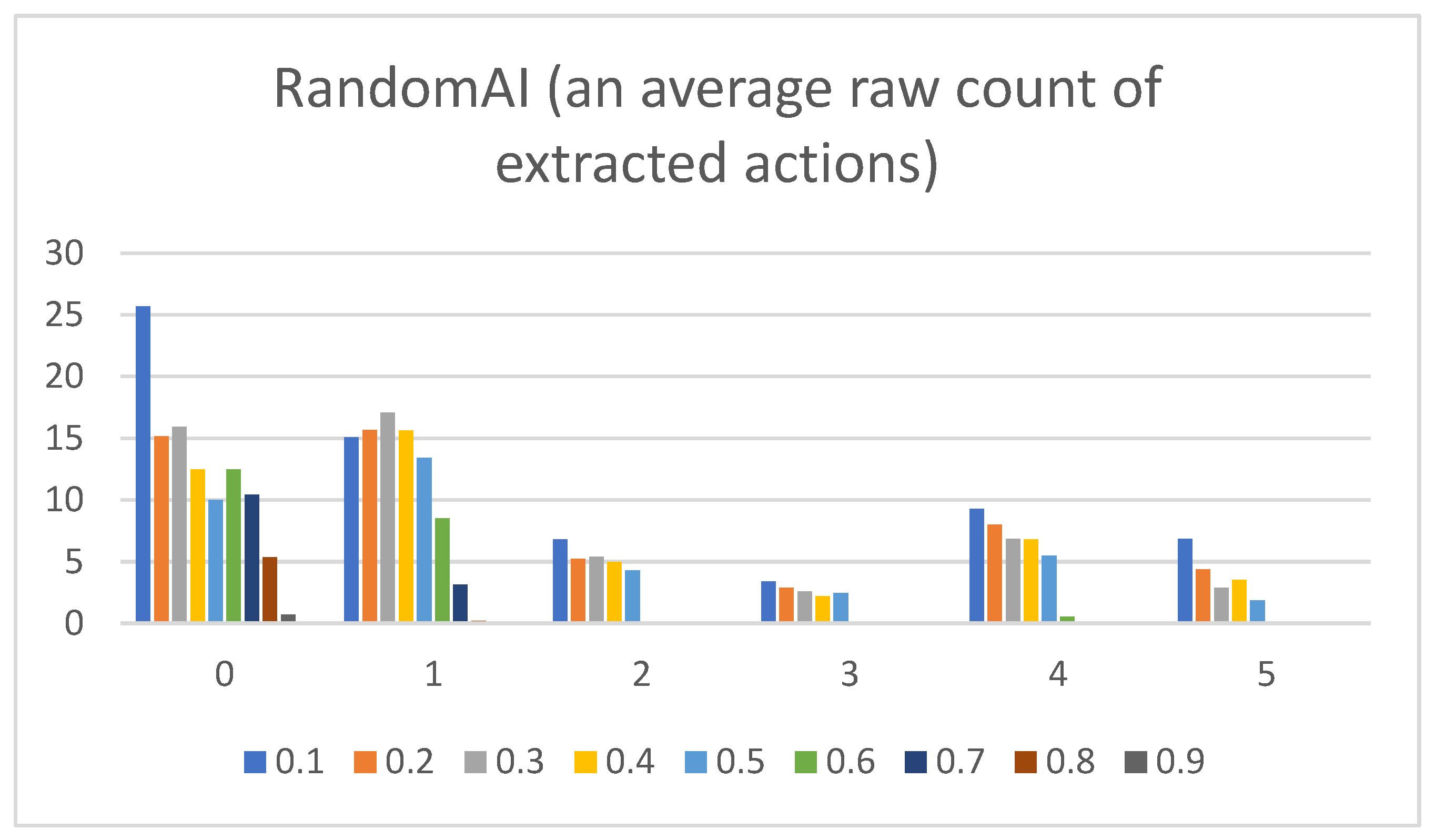
• There are, in total, six game actions in microRTS to be executed by the appropriate units (all are used in the dcARM method): wait (0) (i.e., the unit takes no actions in the current frame), move (1) (i.e., the unit should move to the other cell), harvest (2) (i.e., the unit must gather resources), return (3) (i.e., the unit should return to base with the resources), produce (4) (i.e., the unit must produce another unit) and attack location (5) (i.e., the unit attacks the opponent’s unit at a specific location/cell). Due to the low number of available actions in the microRTS environment, no action abstractions are used (e.g., grouping actions based on specific criteria).
• The chosen features for this experiment, which are gathered from the microRTS game state, are shown in

  Table 3. All features used in the microRTS experiment.

  Feature Acronym	Feature Description
  [fr/op]Worker	The number of Worker units (on the map).
  [fr/op]Light	The number of Light units.
  [fr/op]Heavy	The number of Heavy units.
  [fr/op]Ranged	The number of Ranged units.
  baseThreatFriendly	Are any of the friendly bases under threat (true/false)? The base is under threat if there is an opponent unit present for two physical game map squares in either direction of the base.
  [fr/op]ResourcesLeft	The number of resources left to spend.
  [fr/op]Bases	The number of Bases.
  [fr/op]Barracks	The number of Barracks.

  (the [fr/op] part symbolizes that two distinct features are used: one for the friendly side and one for the opposing side).

• The interval of the following rule confidence thresholds θcv is used: [0.1, 1.0] (with a step of 0.1).
• The maximum passed time for keeping records is set as unlimited (i.e., all rules from the beginning of the game are included).
• The maximum passed time for keeping an AIP is set to unlimited (i.e., all AIPs from the beginning of the game are included).
• The sampling rate is set to one (i.e., the dcARM method is utilized in each game frame).

Five game agents are selected from the set of agents for dcARM method testing. All the agents come pre-included in the microRTS package and are used as-is. The chosen agents represent groups of random, scripted and advanced game tree-based agents. Specifically, RandomAI and RandomBiasedAI (two game agents utilizing baseline random behavior, but with the second game agent being biased toward attack, harvest or return actions), WorkerRush (basic scripted behavior, with the only goal being the construction of Worker game units and rushing/attacking the opponent), UCT (Upper Confidence Bounds applied to game tree) and NaiveMCTS (advanced behavior utilizing a game tree-based internal structure). Note that, when the biased mechanisms in RandomBiasedAI are used, it does not mean that the attack, harvest or return actions, if available, are always utilized (i.e., selected by default). Instead, the implemented bias only lowers the probability of the move action and does not disregard it entirely. The chosen agents always play a game in pairs with a RandomAI agent. After the agent in testing returns a set of actions (note: the 100 milliseconds time slice is not violated), the game pauses for experimentation purposes before iterating to the next frame [41]. Every agent plays ten games for each threshold from the threshold interval.

During the experiment, time measurements are made and recorded for step three of the dcARM method, which is due to the utilization of the nature-inspired DE algorithm, the most complex method step, therefore consuming the highest amount of processing time (i.e., other steps vary very slightly in time execution between frames, so all the focus is directed toward the most time-expensive part of the method).

5.2. Real-Time Strategy Digital Characterization Data Results

Due to the RTS gameplay, game states can occur that come devoid of extracted actions. The presentation of the RTS characterization analysis results also includes such game states. In contrast, for the case study of the RPS game, the blocks empty of actions are omitted from the tables to focus purely on the aspect of actions (i.e., the RPS game example is simple, and it is not necessary to hinder the presentation of the results with any non-action-related information). The RTS results hence show how representative each action is for the whole game. Ultimately, in RTS games, there is a dependency between the chain of game states established (i.e., every game state (except the first one) is a follow-up of the game state that came before it). Therefore, even the game states that are empty of actions contribute to the overall gameplay.

The results of the experiment for all the thresholds (from 0.1 to 1.0) and all the game agents are presented in three graph segments. Each segment corresponds to one of the segments of the AIP abstraction of information:

(a)

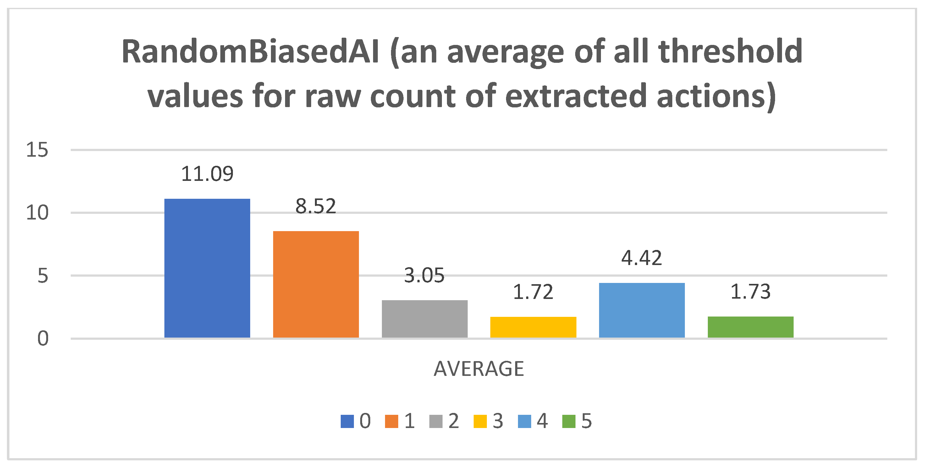
Raw counts of extracted actions. The graphs in Figure 3, Figure 4, Figure 5, Figure 6 and Figure 7 show the raw counts of the extracted actions (i.e., the DC holds the actions averaged across all gameplay frames and also those averaged for all ten games played) (ordinate axis) for each available action (abscissa axis). The figures in Appendix B present a single value for each specific action, because discussing the differences between agents can (sometimes) be more straightforward with just one value. Therefore, the graphs shown in Figure A1, Figure A2, Figure A3, Figure A4 and Figure A5 show the average value across all thresholds (ordinate axis) for each specific action (abscissa axis). Note, however, that some thresholds with a (near) zero value can substantially lower the overall value, making interpretations with only one value more difficult due to less information.

(b)

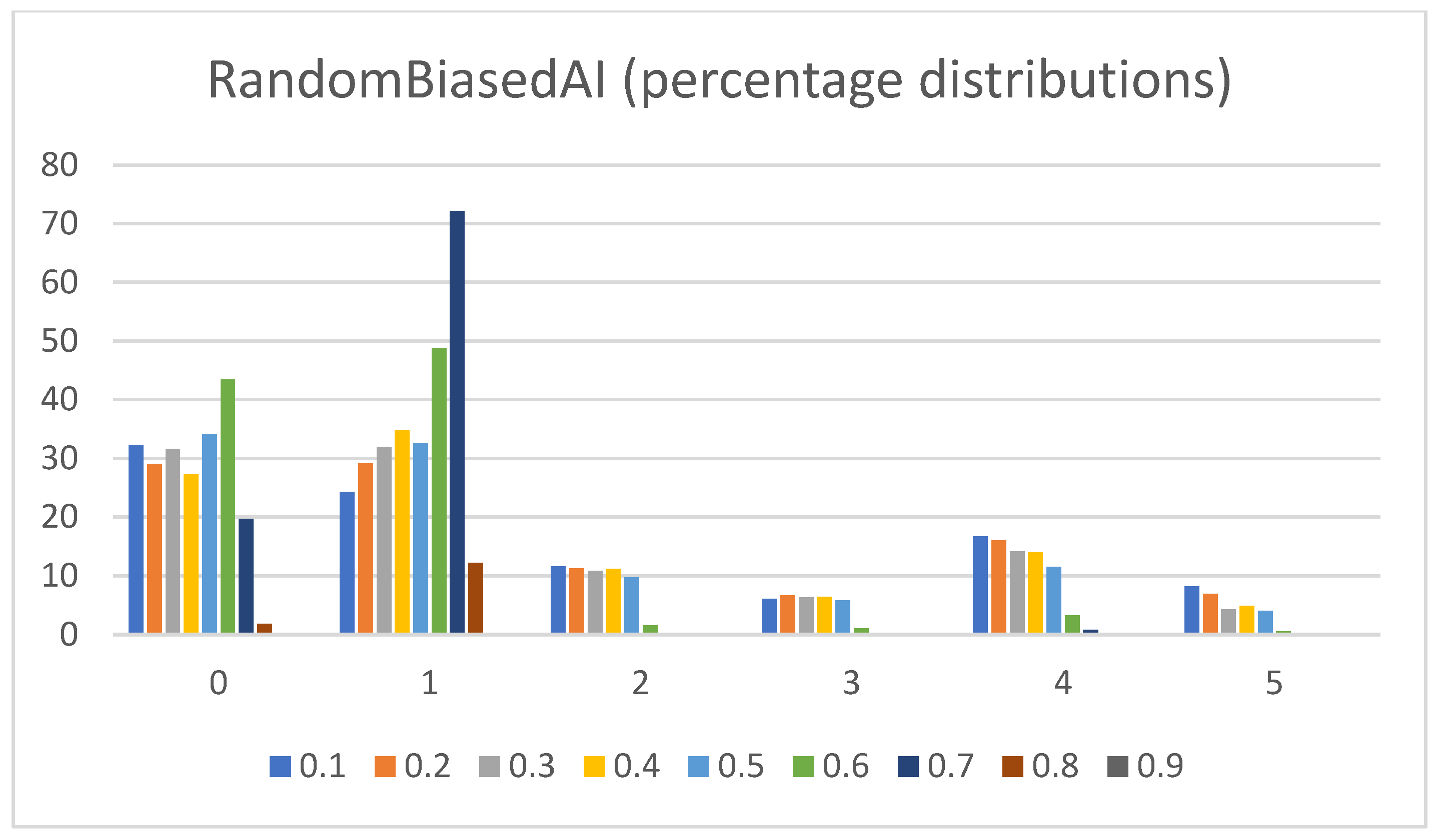
Percentage distributions of extracted actions. The graphs in Figure 8, Figure 9, Figure 10, Figure 11 and Figure 12 show the percentage distributions of the extracted actions (i.e., the DC holds the actions averaged across all gameplay frames, and also those averaged for all ten games played) (ordinate axis) for each available action (abscissa axis).

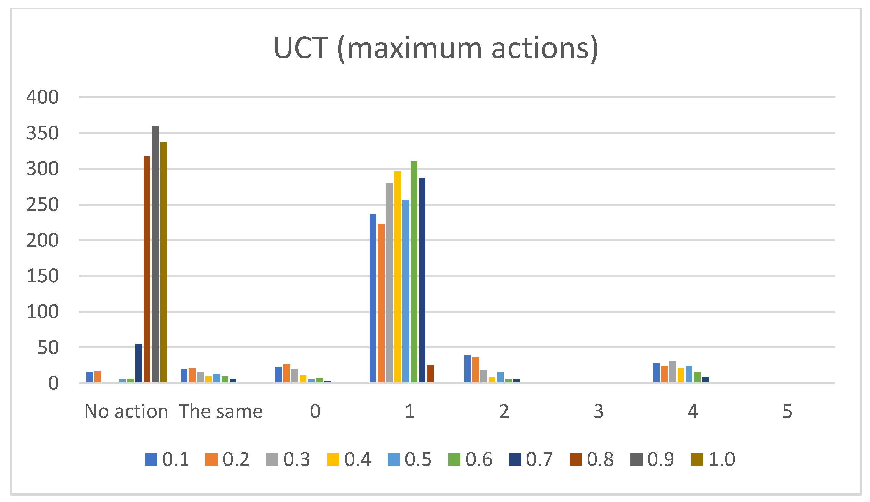
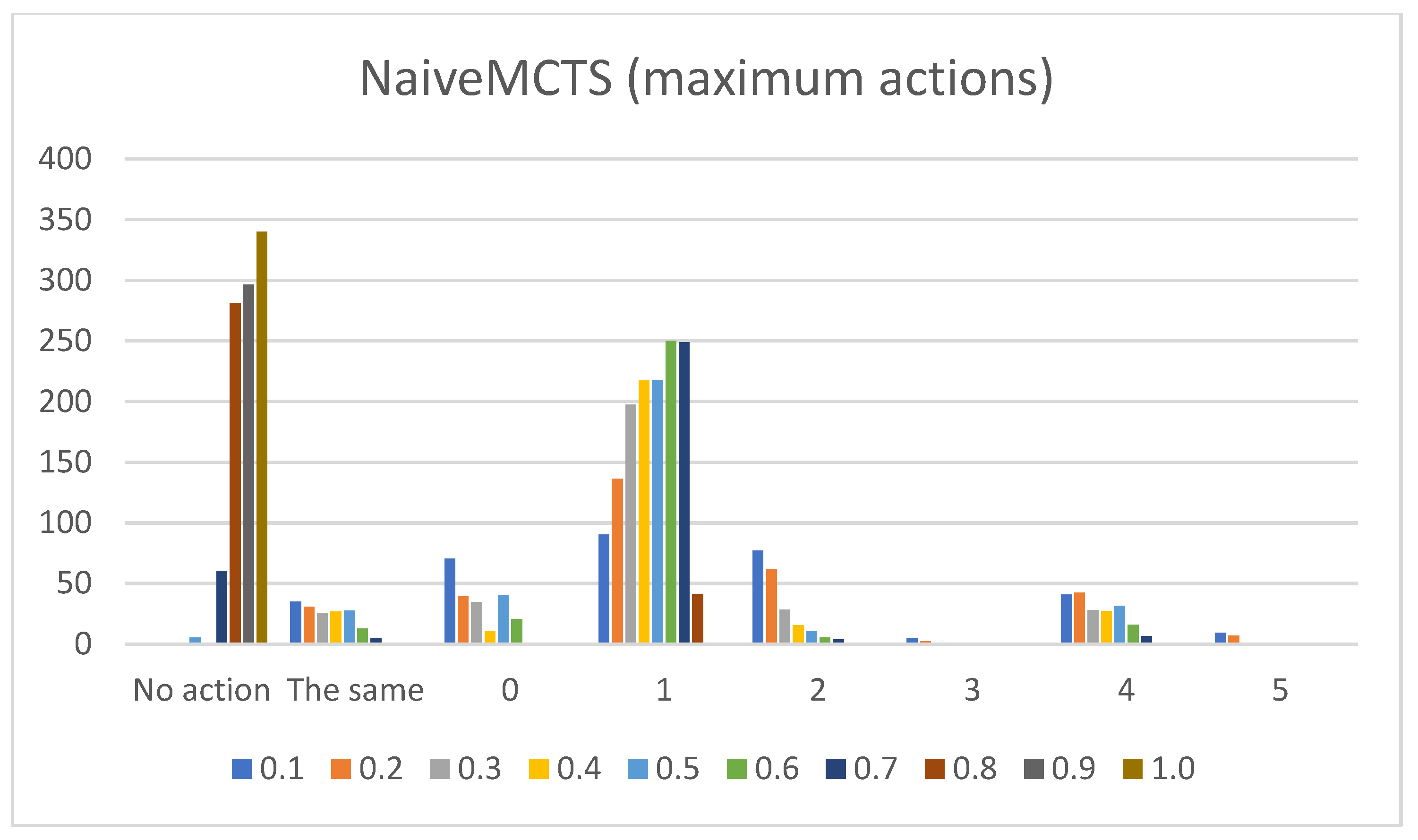
(c)

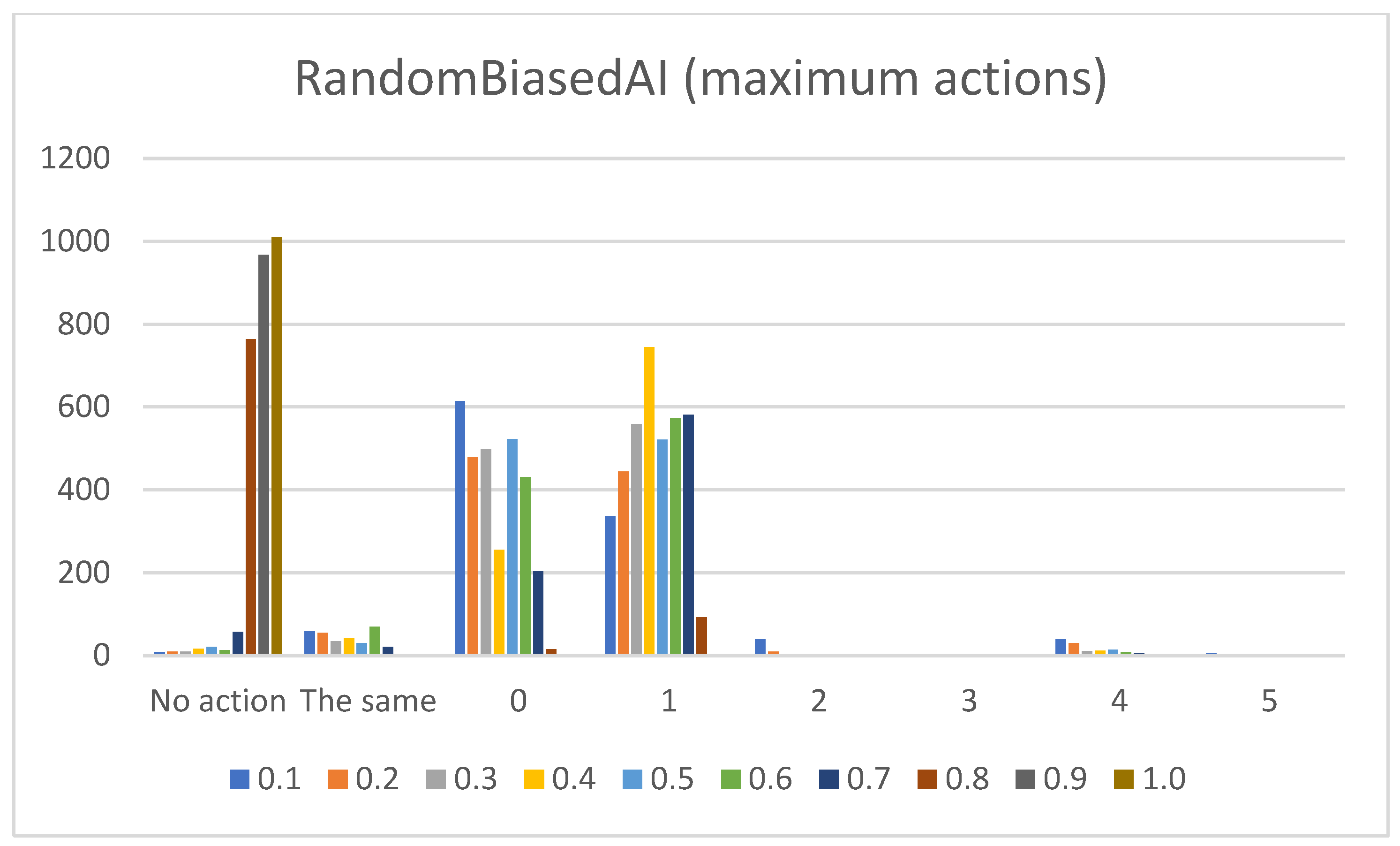
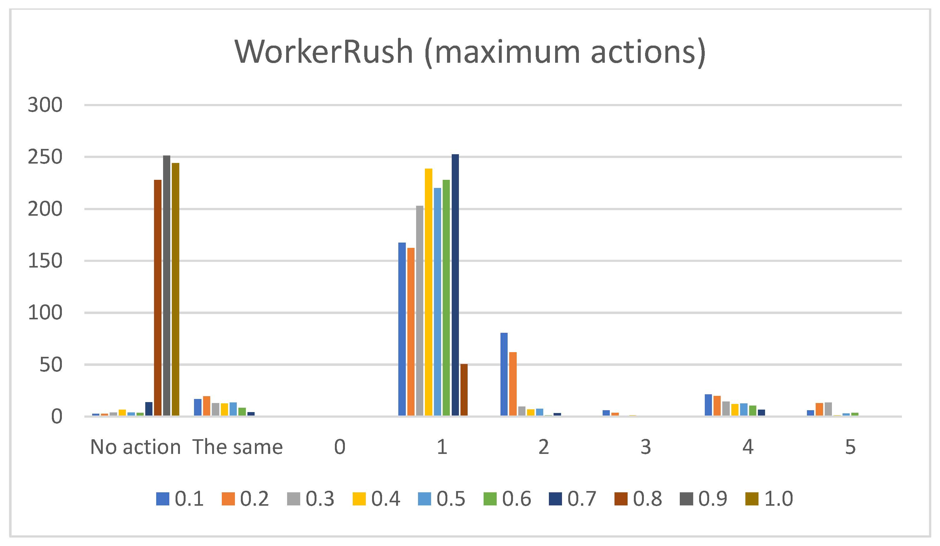
Sum of maximum actions. The graphs shown in Figure 13, Figure 14, Figure 15, Figure 16 and Figure 17 show the counts of achieving the maximum action (i.e., the DC holds the maximum actions summed across all the gameplay frames, and also those averaged for all ten games played) (ordinate axis) for each available action (abscissa axis). Note: The graphs for the maximum actions include two additional labels named “No action” and “The same”, which stand for how many times no action is taken (i.e., if no action is taken, then there is no maximum action), and how many times two or more actions reach the same maximum action status (i.e., they havve the same maximum percentage distribution).

5.3. Time Data Results

The time data recorded during the dcARM method execution of ARM in step three is presented in this section. This analysis is performed to establish how much time is needed while running the most demanding part of the method in a complex RTS game environment. Such an analysis should present a narrative of how the time measurements fit in the reactive control, tactical and strategic time intervals identified in the related work.

The graphs shown in Figure 18, Figure 19, Figure 20, Figure 21 and Figure 22 show the time in milliseconds (ordinate axis) required to execute ARM at a specific game frame (abscissa axis) for all the games (one hundred in total), for all the thresholds (from 0.1 to 1.0) and for all the game agents. Appendix C is also included to demonstrate (and to better illustrate) how the game-agent-recorded ARM time data behave at a specific threshold. Appendix C contains the graphs from Figure A6, Figure A7, Figure A8, Figure A9 and Figure A10 (for five game agents), which show the time in milliseconds (ordinate axis) required to execute ARM at a specific game frame (abscissa axis) during the span of ten games for a threshold of 0.5.

6. Discussion

This section is divided into four parts. First, the DC results of the five game agents used in the experiment are discussed and summarized first. Second, the suitability of the dcARM method is upheld for real-time game usage. Third, three possible directions for future research are presented. Last, the possible drawbacks of the method are provided, and suggestions are given for improvements.

6.1. DC Results of Five Game Agents

In the following list, a short discussion and summary of the DC results are provided for every game agent used in the experiment.

(a)

RandomAI/RandomBiasedAI:

Pretext: Both agents share the same core (i.e., random behavior), which is clearly shown on their graphs due to their similarity. Both agents are also very keen on using the wait (0) and move (1) actions.

Presentation of results: The average raw count of the extracted wait (0) action for both agents shows values of around 13 to 16, whereas those of UCT and NaiveMCTS are much lower at around 8 to 10. For the move (1) action, the count is similar between the agents but with slightly lower values when compared to those of other agents (i.e., around 15, whereas other agents are a few points above this).

When the percentage graphs are observed, the usage of the wait (0) action is maintained at around the 30 percent mark (with those of UCT and NaiveMCTS being much lower, at around 18 percent).

In the maximum action graphs, the wait (0) and move (1) actions surpass a count of 1000 (even reaching 1500 in some cases) for the RandomAI agent, and the RandomBiasedAI has them at around 500 to 600. Every other agent has a much lower value for the maximum action count for these two actions (only that of UCT reaches the 300 mark for the move (1) action).

For the remainder of the actions, only the produce (4) action is shown slightly in the graphs, and the return (3) and attack location (5) actions are not used.

Summary: The wait (0) action is used less by other agents, which signals that they utilize much more intelligence- (i.e., actions with active purposes) driven behavior than these two agents do. Even the usage of “No action taken” is, for these two agents, up to three times higher than that for any other agent.

(b)

WorkerRush:

Pretext: This rushing agent expresses the most apparent result of a clear-cut connection between the game agent’s DC and the agent’s actual modus operandi. The agent graphs show that the wait (0) action is not utilized, whereas every other agent at least considers using it.

Presentation of results: The averaged raw count of the extracted move (1) action is on par with those of the other agents (even slightly higher than those of the RandomAI and RandomBiasedAI). The harvest (2) action count candles are mainly represented at around mark eight (slightly lower than those of the UCT and NaiveMCTS agents). The return (3) action is stable at mark five (somewhat higher than those for the UCT and NaiveMCTS agents). The produce (4) action is on par with that of the UCT agent (for some candles, it is even higher) at around mark eight but is lower than that of the NaiveMCTS agent. The attack location (5) action is very similar to those of the other agents.

When the percentage graphs are observed, the move (1) action is the most represented action among all agents (and the graphs regarding this action are also similar), but the candles for the WorkerRush and UCT agents are around ten percent higher. The harvest (2) action is twice as high for the WorkerRush, UCT and NaiveMCTS agents compared those of the RandomAI and RandomBiasedAI agents. The produce (4) action for this agent is similar to that of NaiveMCTS at around twenty percent. This is the highest compared to the other agents, which are mainly found in the twelve to fourteen percent range. The attack location (5) action does not deviate considerably compared to those of the other agents.

Regarding the maximum action graphs, the “No action taken” candles are the lowest among all the agents. The candles for other actions are similar to those of the NaiveMCTS agent. The maximum actions for the return (3) and attack location (5) actions show slightly higher behavior for this agent (i.e., in comparison to other agents, whose candles are almost non-existent).

Summary: Because the primary operation of the WorkerRush agent is rushing the opponent, its DC clearly shows that the agent has no use for waiting. The agent’s harvesting behavior is twice as high as those of the random-based agents and is similar to those of the other two competent agents, signaling intelligent/scripted (i.e., non-random) behavior. The same can be stated for the utilization of returning actions (i.e., it is distinct from random behavior). Production is very high on this agent’s agenda, which is to be expected, because the agent’s primary purpose is to rush the opponent with as many units as possible.

(c)

UCT:

Pretext: The UCT agent is quite a capable agent, and its behavior lies somewhere along the lines of NaiveMCTS but with more balanced behavior (e.g., the candle sizes do not show as much of a decline between the different thresholds in the averaged raw action count when compared to those of WorkerRush or NaiveMCTS).

Presentation of results: For this agent, the presentation is kept short because most of the results are already discussed in the actions of the previous agents. To summarize, the averaged raw action counts and percentage distributions for the wait (0) action are similar to those of the NaiveMCTS agent (i.e., in the vicinity of mark eight for a raw count and around 18 percent for percentage distributions), and the maximum actions count is almost half in comparison to that of the same agent. For the move (1) and harvest (2) actions, the graphs show similar behavior to those of the WorkerRush and NaiveMCTS agents. The return (3) action is slightly less well represented than those of WorkerRush and NaiveMCTS (e.g., the percentage distributions are below ten percent, whereas these two agents have them firmly on ten percent). The produce (4) action is almost half (e.g., in terms of percentage distributions) compared to those of other agents, and is on par with RandomAI. The attack location (5) action numbers are similar to those of the NaiveMCTS agent.

Summary: This agent is balanced across actions and is not too keen on production. Its actions are similar to those of NaiveMCTS but with slightly lower action counts.

(d)

NaiveMCTS:

Pretext: It is interesting to observe how this agent’s DC comes close to the DC of the WorkerRush agent (except for the wait (0) action, which is almost non-existent in WorkerRush). This behavior could be attributed to both agents utilizing aggressive tactics against the opponent.

Presentation of results: The NaiveMCTS action results are already presented when describing other agents. This agent utilizes the production (4) action quite heavily (i.e., a twenty percent distribution of choosing this output is quite intensive for an RTS game).

Summary: This agent drives a very offensive-oriented game, which is quite evident when compared to the DC of the WorkerRush agent (also offensive-oriented).

The data results present a comprehensive picture across specific actions and reveal the DC similarity patterns (e.g., similar offensive behaviors for NaiveMCTS and WorkerRush), as well as crucial differences (e.g., low values of wait (0) actions for non-random agents) between the agents. Such patterns are an excellent indicator of the DC being a helpful tool when researching explainable agents (e.g., agents that do not allow access to the internal code—black box concept), when trying to compare the agents with each other (e.g., possible classification of agents) or when the characterization is needed for (but not limited to) gameplay purposes (e.g., opponent modeling).

The results also show the importance of different abstractions of the action data. For example, if only the maximum action usages are observed, it would seem as though the agents never use the return (3) and attack location (5) actions. However, when the averaged raw count of extracted actions and percentage distributions are taken into consideration, one can observe that they are indeed used (even up to ten percent with WorkerRush).

6.2. Suitability of dcARM Method for In-Game Usage

In related work, the following time intervals are found for each of the three primary RTS hierarchy abstraction levels responsible for issuing commands to units: a one-second interval for reactive control (unit micromanagement), an interval ranging from thirty to sixty seconds for tactical operations and an interval of approximately three or more minutes for the strategical level. These levels offer the basis for establishing the suitability of the dcARM method’s most time-expensive part (i.e., step three) for in-game usage. A reminder of the experiment’s settings is as follows: the method’s use for this experiment is at an intensive peak due to keeping the recorded data of all previous frames and with all frames sampled (i.e., the sampling rate is set to one).

The graphs shown in Figure 18, Figure 19, Figure 20, Figure 21 and Figure 22 reveal the following:

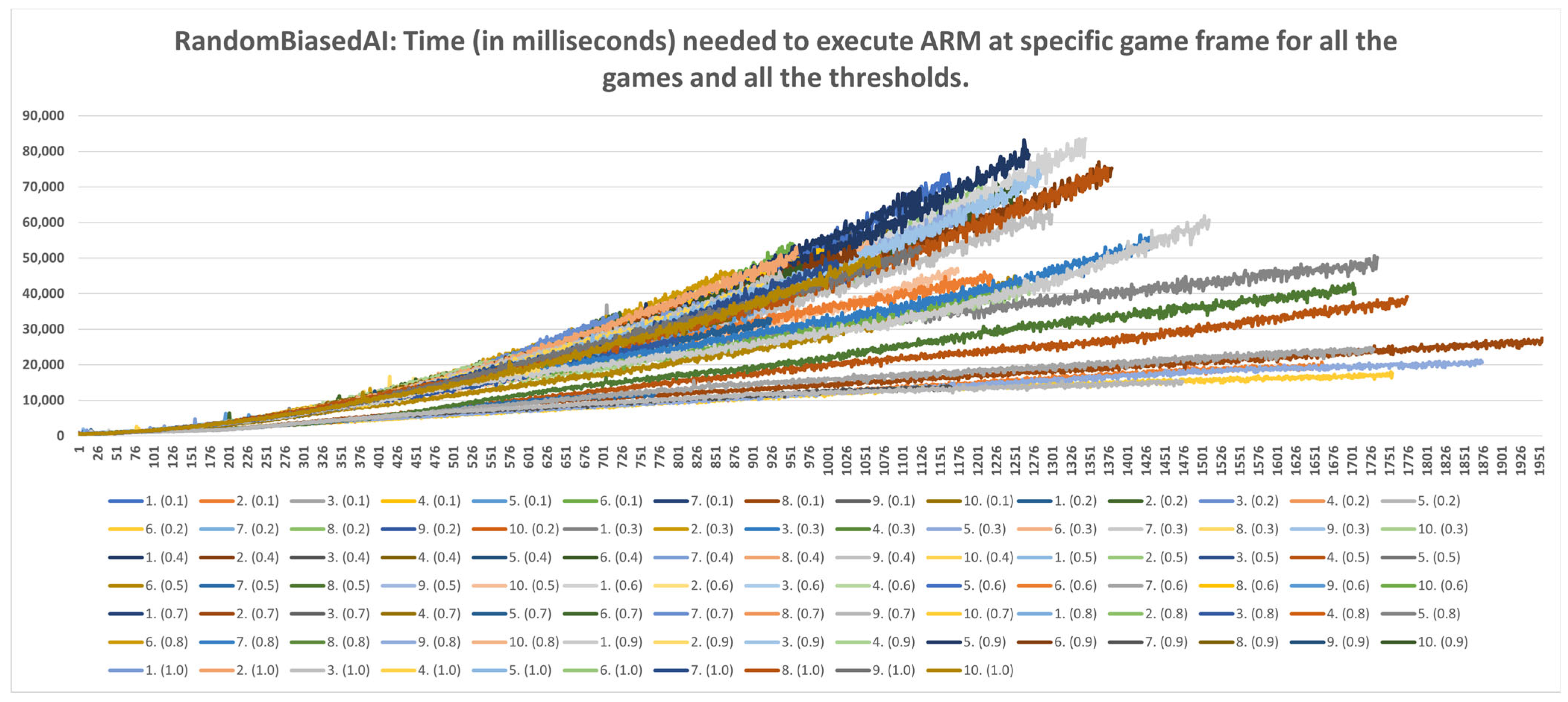
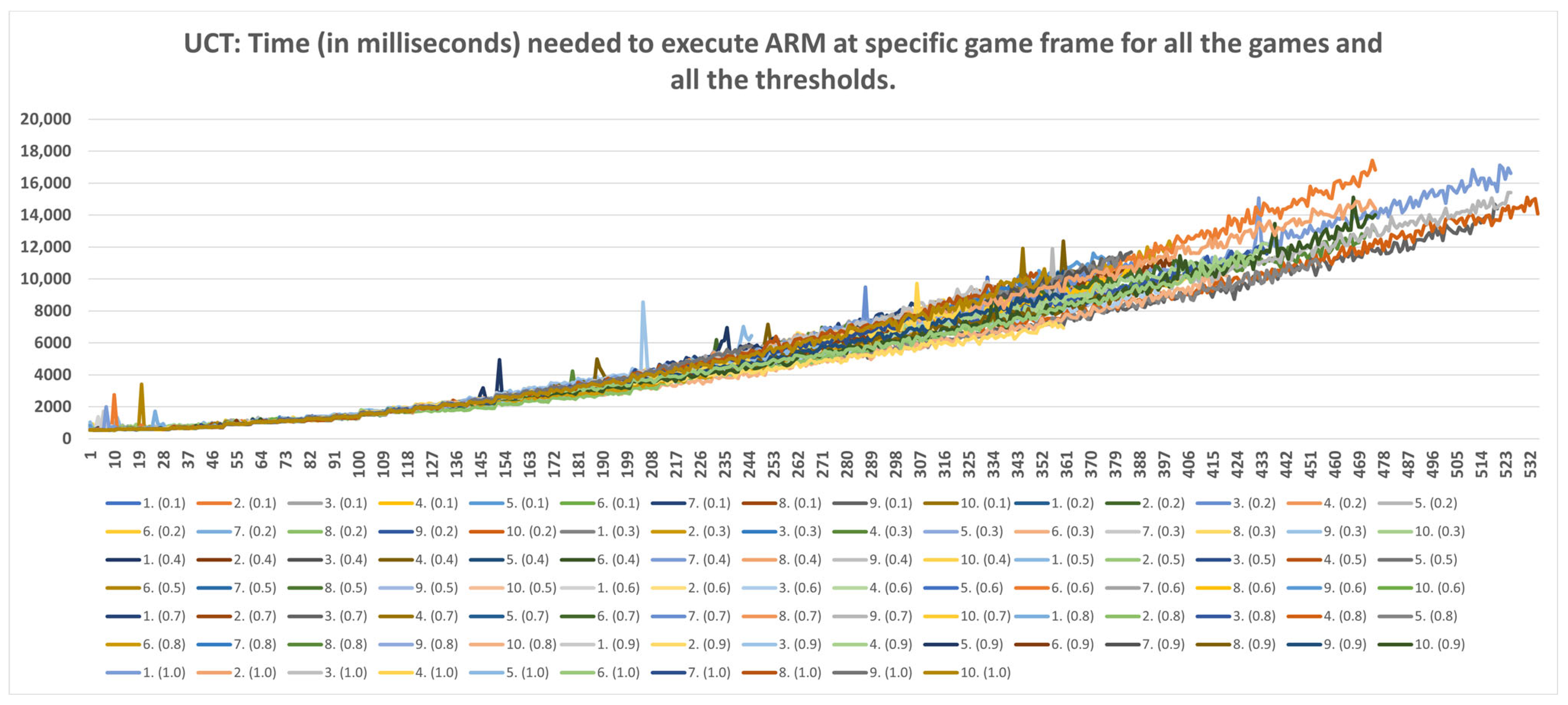
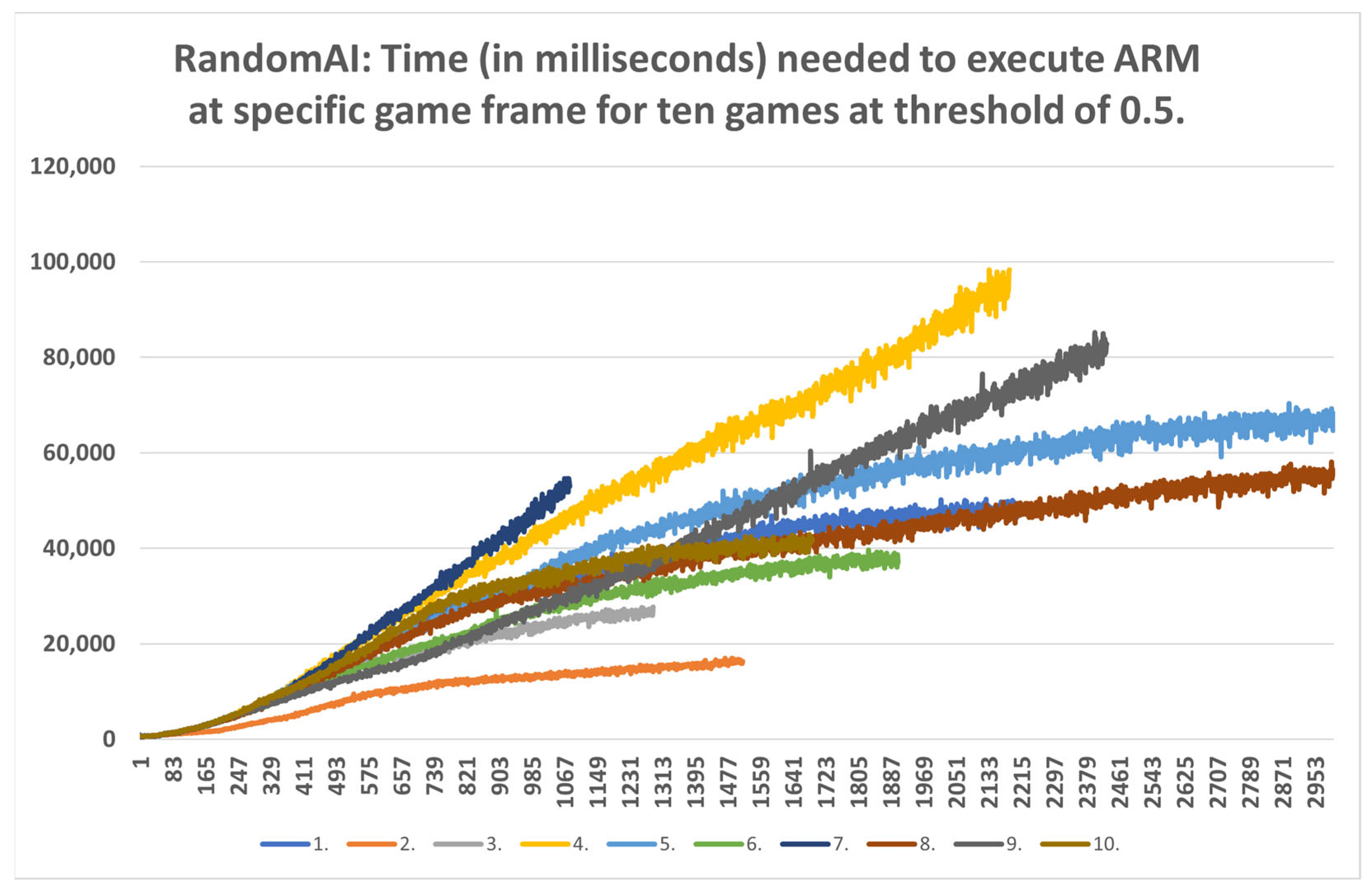
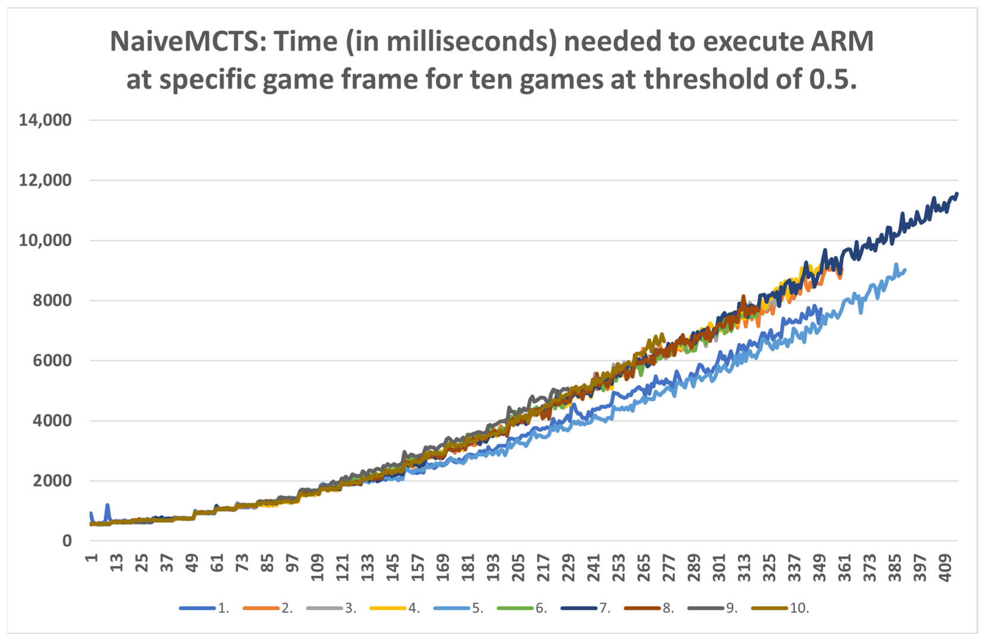
• Strategic level: This method can be used for strategic purposes, because, even with the highest time consumption of RandomAI, there is only one occurrence in which time consumption extends beyond the two-minute mark. RandomAI and RandomBiasedAI are otherwise the most time-consuming agents due to playing the longest games (i.e., measured by the overall frame count). For the other agents, the highest time consumptions are at around eighty seconds (RandomBiasedAI), nine seconds (WorkerRush), fifteen seconds (UCT) and eleven seconds (NaiveMCTS).
• Tactical operations: Regarding the timings of tactical operations, the usage of this method is also possible for every non-random agent (i.e., their measured time values are a lot lower than the sixty-second limit) and for the random agents (i.e., the method could be used to approximate the inclusion of up to a thousand frames).
• Micromanagement purposes: Some time restrictions must apply when building the DC for micromanagement purposes. For example, if non-random agents are observed, the one-second mark is passed at approximately fifty frames. Moreover, if the first fifty frames of the games are followed, the time increases almost linearly. However, later on, the time data grow in a non-linear way, and therefore the number of frames used for micromanagement should be lower. For example, in later stages of the UCT agent games, the graph in Figure A9 can easily increase by two seconds in fifty frames.

6.3. Possible Directions for Future dcARM Research

This subsection presents three possible directions for further DC research.

6.3.1. Automated Game Policy Creations

Nuances, or harder-to-spot differences in action abstraction values, can occur in the data. Such nuances can hold vital information regarding what kind of plan the game agent is pursuing. For example, the DC data for the WorkerRush and NaiveMCTS agents are very similar for some actions (e.g., the percentage distributions for production were similar) but completely different in other regards (e.g., the action related to waiting is not utilized in WorkerRush, whereas NaiveMCTS uses it at around eighteen percent, when the non-zero threshold candles are observed). Therefore, different actions can be grouped (possibly automatically) to form the (strategic) game policy (or the game-specific aspect the agent is pursuing). Multiple game policies (e.g., for different aspects of the RTS game, such as production or combat) can also serve as descriptions of the game agent. They can also be incorporated into the DC as higher-level descriptions.

For policy creation, we envision a method that creates the action-based game policy automatically (i.e., selecting and combining actions to form a policy while considering the AIP’s action abstraction levels). Automatic machine learning (known as autoML [42]) can be utilized first to create a selection of game-policy-specific features (feature engineering can be utilized to lower the complexity of dcARM usage). Second, the responding DC can be constructed, and last, the game policy (or multiple policies) can be created, consisting of actions that are above some (pre-set) thresholds for AIP’s action abstraction values. However, because such research is out of the scope of the current paper, we leave it for future research.

6.3.2. Usage of DC for Future Simulation Purposes

When executing the steps from 2 to 5 in the dcARM method, a new AIP data point is created on the game frame (time) interval. This point covers the interval frame sequence from the previous point up to this point. By analyzing the differences in AIPs between the points, changes in player behavior can be detected (e.g., changes in the opponent model). Differences between the AIPs should also allow for determining what game policies the player uses during specific time intervals (i.e., not only the game policies for the whole game, but possible (sub)game policies for specific (sub)time intervals).

By following the changes in the opponent’s action behavior across time and the usage of (sub)policies, it may be possible to make predictions regarding how the opponent behaves in the future, or to test (e.g., by simulating computer-controlled players in advance) whether the actions of another player can alter the behavior (i.e., influence the DC) of the player under observation. Such predictions open up a variety of options for future simulation purposes. For example, a simulation can be made with specific actions executed against the opponent to determine whether the opponent’s DC adjusts accordingly, revealing their weak spots. On the other hand, if the player’s DC does not change, this may signal that the player is perhaps scripted (non-adaptive). In addition, by focusing on action simulations (i.e., only a few actions of the action set are selected based on the chosen DC action value criteria), benefits in lowering simulation complexities can be achieved due to not using randomness across the set of all actions.

6.3.3. DC as the Driver of a Game Agent’s Decision Process

One of the future research viabilities for DC may lie in it being a contributing factor to the game agent’s decision process, whereas other techniques, components and algorithms require additional confirmation as to whether the chosen actions are suitable for the opponent at play. For example, if the decision process has multiple scenarios created (e.g., of equal probability to be selected) on how to approach the gameplay in the near future, and if it knows that the DC of the player is very offensive, it would likely be wiser to use a counter-offensive scenario than to go with the unit-research scenario and, in the process, losing the game. The opponent’s action behavior (i.e., with patterns of AIPs) across different game time points provided in real-time can also act as feedback on how well or poorly the scenario is being acted out.

6.4. Drawbacks of the Method and Room for Improvement

However, there are some drawbacks of this approach and possible improvements to be made to the dcARM method, which must be addressed in the future.

• DC offers many different abstractions of data, which, when combined with multiple threshold possibilities, a sampling rate and a large set of actions, creates many possible DC variations (patterns). Such patterns hold subtle clues, which are sometimes only revealed when observed under the right action abstraction, or when there is knowledge of exactly what is being searched for (e.g., if the agent is frequently moving, this can be an essential clue when researching micromanagement). DC patterns can also capture the character abstraction from the macro picture (e.g., an agent is keen on production), but more refinement to the method is needed to capture the micro picture (i.e., hard-to-spot nuances). For example, one can quickly identify when the agent is keen on a specific action. However, minor differences (e.g., of one percent) in action usage can mean a different utilization of such action. For example, two agents exhibit similar patterns for some behaviors, as NaiveMCTS and WorkerRush agents do for production, but otherwise have entirely different background implementations, tactics and strategies. Such nuances are observed very nicely in the RPS case study, where even a ten percent bias toward a specific action is captured with definitive conclusions. However, RTS environments are very complex, and in-depth research on the capability of DCs is needed in the future to obtain even more definitive answers (or better resolution) regarding the (in-depth) agents’ behavior.
• Automatic feature engineering [14] is focused on in step 1 of the dcARM method. Therefore, only the features that represent the game agent correctly and contribute significantly to the relevant DC construction (i.e., the DC of the game agent is of high confidence due to the usage of quality features) should be automatically selected. This would be a substantial improvement because the dcARM method would be completely automated. To achieve this goal, the utilization of deep learning simulation environments [43] and deep learning methods [44] is on our research agenda.
• In the current work, the game is paused during the frames to allow for the uninterrupted execution of the dcARM method, and to gather all the data needed for different types of analyses. For example, lessons learned with time analysis can help enhance the method to be time-adjustable in the future, allowing it to be incorporated into the game agent’s lifecycle. In this way, part of the game agent’s time slice can be allocated to the method, helping the agent’s decision making through DC data utilization into better capabilities with which actions to play.
• Data-squashing methods [45] can be used on the dcARM method input feature datasets, which can reduce the time needed to execute the dcARM method.

Although this subsection focuses on the drawbacks of the method, we finish with an advantage of DC. With access to game engine APIs (i.e., application programming interfaces), one can always determine the set of available actions. If access to such a set is not possible, the available set of actions can be determined by playing the game. Therefore, the main aspect required for creating a DC is (almost always) available from the start, opening the doors for the dcARM method’s usage across many game environments (i.e., usage possibilities are opened up for non-RTS games as well).

7. Conclusions

In this article, the practicality of using DC is shown across the initial RPS case study experiment as well as with a more complex experiment positioned in the RTS game environment. The results of the initial case study confirm our expectation that even a slight bias toward specific actions would be clearly shown in the data. The complex experiment positioned in the RTS game environment further reveals that having a set of different action abstractions within the AIPs can be imperative when searching for specific nuances of player behaviors.

The data interpretation of the five game agents confirms that such nuances are present. It is demonstrated that random-based agents show a lack of active, purpose-driven behavior, highlighted by their frequent use of waiting and the “No action taken” option, whose usage is up to three times higher than that of any other agent. WorkerRush’s complete absence of waiting behavior is in line with its scripted rushing agenda. Its production behavior is very high, which is also in line with the purpose of rushing the opponent with as many units as possible. The harvesting and returning nuances are similar to more advanced agents. For the UCT agent, the data show balanced behavior across all actions without prioritizing production. NaiveMCTS prioritizes production and drives a very offensive-oriented game.

Another example of how DC interpretations can be helpful is by observing changes in action percentages across time, which can reveal the tactics and strategies of a player. Moreover, having maximum action information can be turned into an advantage, because, if one knows that a player is overusing some specific action, there are multiple ways to utilize such behavior to our own benefit. Thus, by using different action abstractions, game behavior patterns can be created, game policies that the player is applying can be revealed, or the DCs can be used for future simulation purposes (as outlined in Section 6.3). In future work, such research directions will be explored further, with each direction’s automatic (or intelligent) element being one of the top priorities.

To conclude, game spaces are continually increasing in complexity. One merely must remember the look of arcade games from the nineteen-seventies and -eighties and compare them to the newest game engines with almost photorealistic graphics to see that it is evident that the trend in complexity will only continue. Therefore, the need to know how (unknown) game (engine) components operate is high (i.e., gaining deeper insight into the operation of “black boxes”). Through creating component abstractions, patterns, models and now DCs with the help of powerful optimization-based tools, the field of explainable AI can, hopefully, be advanced, improvements to (or an increased understanding regarding) the gameplay can be made, and the path to a new era of video games can be set (e.g., metaverse games [46]).

References

- Levy, L.; Lambeth, A.; Solomon, R.; Gandy, M. Method in the madness: The design of games as valid and reliable scientific tools. In Proceedings of the 13th International Conference on the Foundations of Digital Games, Malmö, Sweden, 7–10 August 2018; pp. 1–10. [Google Scholar] [CrossRef]
- Isaksen, A.; Gopstein, D.; Nealen, A. Exploring Game Space Using Survival Analysis. In Proceedings of the International Conference on Foundations of Digital Games, FDG 2015, Pacific Grove, CA, USA, 22–25 June 2015. [Google Scholar]
- Prensky, M. Fun, play and games: What makes games engaging. Digit. Game-Based Learn. 2001, 5, 5–31. [Google Scholar]
- Goel, A.K.; Rugaber, S. Interactive meta-reasoning: Towards a CAD-like environment for designing game-playing agents. In Computational Creativity Research: Towards Creative Machines; Atlantis Press: Paris, France, 2015; pp. 347–370. [Google Scholar] [CrossRef]
- Adil, K.; Jiang, F.; Liu, S.; Jifara, W.; Tian, Z.; Fu, Y. State-of-the-art and open challenges in RTS game-AI and Starcraft. Int. J. Adv. Comput. Sci. Appl. 2017, 8, 16–24. [Google Scholar] [CrossRef]
- Butler, S.; Demiris, Y. Partial observability during predictions of the opponent’s movements in an RTS game. In Proceedings of the 2010 IEEE Conference on Computational Intelligence and Games, IT University of Copenhagen (ITU), Copenhagen, Denmark, 18–21 August 2010; pp. 46–53. [Google Scholar] [CrossRef]
- Novak, D.; Fister, I., Jr. Adaptive Online Opponent Game Policy Modeling with Association Rule Mining. In Proceedings of the IEEE 21st International Symposium on Computational Intelligence and Informatics, Budapest, Hungary, 18–20 November 2021. [Google Scholar] [CrossRef]
- Kerr, B.; Riley, M.A.; Feldman, M.W.; Bohannan, B.J. Local dispersal promotes biodiversity in a real-life game of rock–paper–scissors. Nature 2002, 418, 171–174. [Google Scholar] [CrossRef] [PubMed]
- Dockhorn, A.; Saxton, C.; Kruse, R. Association Rule Mining for Unknown Video Games. In Fuzzy Approaches for Soft Computing and Approximate Reasoning: Theories and Applications; Springer: Cham, Switzerland, 2021; pp. 257–270. [Google Scholar] [CrossRef]
- Levine, J.; Congdon, C.B.; Ebner, M.; Kendall, G.; Lucas, S.M.; Miikkulainen, R.; Schaul, T.; Thompson, T. General video game playing. In Artificial and Computational Intelligence in Games. Dagstuhl Follow-Ups; Dagstuhl Publishing: Dagstuhl, Germany, 2013; Volume 6. [Google Scholar] [CrossRef]
- Uriarte, A.; Ontanón, S. Combat models for RTS games. IEEE Trans. Games 2017, 10, 29–41. [Google Scholar] [CrossRef]
- Dockhorn, A.; Hurtado-Grueso, J.; Jeurissen, D.; Xu, L.; Perez-Liebana, D. Game State and Action Abstracting Monte Carlo Tree Search for General Strategy Game-Playing. In Proceedings of the 2021 IEEE Conference on Games (CoG), Copenhagen, Denmark, 17–20 August 2021; pp. 1–8. [Google Scholar] [CrossRef]
- Ontanón, S.; Synnaeve, G.; Uriarte, A.; Richoux, F.; Churchill, D.; Preuss, M. A survey of real-time strategy game AI research and competition in StarCraft. IEEE Trans. Comput. Intell. AI Games 2013, 5, 293–311. [Google Scholar] [CrossRef]
- Jeerige, A.; Bein, D.; Verma, A. Comparison of deep reinforcement learning approaches for intelligent game playing. In Proceedings of the 2019 IEEE 9th Annual Computing and Communication Workshop and Conference (CCWC), Las Vegas, NV, USA, 7–9 January 2019; pp. 366–371. [Google Scholar] [CrossRef]
- Lara-Cabrera, R.; Cotta, C.; Fernández-Leiva, A.J. A review of computational intelligence in RTS games. In Proceedings of the 2013 IEEE Symposium on Foundations of Computational Intelligence (FOCI), Singapore, 16–19 April 2013; pp. 114–121. [Google Scholar] [CrossRef]
- Richoux, F.; Uriarte, A.; Baffier, J.F. Ghost: A combinatorial optimization framework for real-time problems. IEEE Trans. Comput. Intell. AI Games 2016, 8, 377–388. [Google Scholar] [CrossRef]
- Takino, H.; Hoki, K. Human-Like Build-Order Management in StarCraft to Win against Specific Opponent’s Strategies. In Proceedings of the 2015 3rd International Conference on Applied Computing and Information Technology/2nd International Conference on Computational Science and Intelligence, Okayama, Japan, 12–16 July 2015; pp. 97–102. [Google Scholar] [CrossRef]
- Stanescu, M.; Barriga, N.A.; Buro, M. Hierarchical adversarial search applied to real-time strategy games. In Proceedings of the Tenth Artificial Intelligence and Interactive Digital Entertainment Conference, North Carolina State University, Raleigh, NC, USA, 3–7 October 2014. [Google Scholar]
- Marino, J.R.; Moraes, R.O.; Toledo, C.; Lelis, L.H. Evolving action abstractions for real-time planning in extensive-form games. In Proceedings of the AAAI Conference on Artificial Intelligence, Honolulu, HI, USA, 27 January 2019–1 February 2019; Volume 33, pp. 2330–2337. [Google Scholar] [CrossRef]
- Barriga, N.A.; Stanescu, M.; Buro, M. Game tree search based on nondeterministic action scripts in real-time strategy games. IEEE Trans. Games 2017, 10, 69–77. [Google Scholar] [CrossRef]
- Churchill, D.; Buro, M. Hierarchical portfolio search: Prismata’s robust AI architecture for games with large search spaces. In Proceedings of the Eleventh Artificial Intelligence and Interactive Digital Entertainment Conference, University of California, Santa Cruz, CA, USA, 14–18 November 2015. [Google Scholar]
- Ontanón, S.; Synnaeve, G.; Uriarte, A.; Richoux, F.; Churchill, D.; Preuss, M. RTS AI Problems and Techniques. Encycl. Comput. Graph. Games 2015, 1, 1–12. [Google Scholar] [CrossRef]
- Palma, R.; Sánchez-Ruiz, A.A.; Gómez-Martín, M.A.; Gómez-Martín, P.P.; González-Calero, P.A. Combining Expert Knowledge and Learning from Demonstration in Real-Time Strategy Games. In Proceedings of the International Conference on Case-Based Reasoning, London, UK, 12–15 September 2011; Springer: Berlin/Heidelberg, Germany, 2011; pp. 181–195. [Google Scholar] [CrossRef]
- Yang, P.; Roberts, D.L. Extracting human-readable knowledge rules in complex time-evolving environments. In Proceedings of the International Conference on Information and Knowledge Engineering, The Steering Committee of The World Congress in Computer Science, Computer Engineering and Applied Computing (WorldComp), Las Vegas, NV, USA, 22–25 July 2013. [Google Scholar]
- Wang, L. Discovering phase transitions with unsupervised learning. Phys. Rev. B 2016, 94, 195105. [Google Scholar] [CrossRef]
- Kantharaju, P.; Ontañón, S. Discovering meaningful labelings for RTS game replays via replay embeddings. In Proceedings of the 2020 IEEE Conference on Games (CoG), Osaka, Japan, 24–27 August 2020; pp. 160–167. [Google Scholar] [CrossRef]
- Das, S.; Suganthan, P.N. Differential evolution: A survey of the state-of-the-art. IEEE Trans. Evol. Comput. 2010, 15, 4–31. [Google Scholar] [CrossRef]
- Agrawal, R.; Srikant, R. Fast algorithms for mining association rules. In Proceedings of the 20th International Conference on Very Large Data Bases, Santiago, Chile, 12–15 September 1994; Volume 1215, pp. 487–499. [Google Scholar]
- Zaki, M.J. Scalable algorithms for association mining. IEEE Trans. Knowl. Data Eng. 2000, 12, 372–390. [Google Scholar] [CrossRef]
- Han, J.; Pei, J.; Yin, Y. Mining frequent patterns without candidate generation. ACM Sigmod Rec. 2000, 29, 1–12. [Google Scholar] [CrossRef]
- Fister, I., Jr.; Fister, I. A Brief Overview of Swarm Intelligence-Based Algorithms for Numerical Association Rule Mining. In Applied Optimization and Swarm Intelligence; Osaba, E., Yang, X.S., Eds.; Springer Tracts in Nature-Inspired Computing; Springer: Singapore, 2021; pp. 47–59. [Google Scholar] [CrossRef]
- Fister, I.; Fister, I., Jr. uARMSolver: A framework for Association Rule Mining. arXiv 2020, arXiv:2010.10884. [Google Scholar]
- Fister, I., Jr.; Iglesias, A.; Galvez, A.; Del Ser, J.; Osaba, E.; Fister, I. Differential evolution for association rule mining using categorical and numerical attributes. In Proceedings of the International Conference on Intelligent Data Engineering and Automated Learning, Madrid, Spain, 21–23 November 2018; Springer: Berlin/Heidelberg, Germany, 2018; pp. 79–88. [Google Scholar] [CrossRef]
- Komai, T.; Kim, S.J.; Kousaka, T.; Kurokawa, H. A Human Behavior Strategy Estimation Method Using Homology Search for Rock-Scissors-Paper Game. J. Signal Process. 2019, 23, 177–180. [Google Scholar] [CrossRef]
- Nagatani, T.; Tainaka, K.I.; Ichinose, G. Metapopulation model of rock-scissors-paper game with subpopulation-specific victory rates stabilized by heterogeneity. J. Theor. Biol. 2018, 458, 103–110. [Google Scholar] [CrossRef] [PubMed]
- Komai, T.; Kim, S.J.; Kurokawa, H. Characteristic extraction method of human’s strategy in the Rock-Paper-Scissors game. NCSP 2018, 18, 592–595. [Google Scholar]
- Castro, S.B.; Garrido-da-Silva, L.; Ferreira, A.; Labouriau, I.S. Stability of cycles in a game of Rock-Scissors-Paper-Lizard-Spock. arXiv 2021, arXiv:2107.09383. [Google Scholar] [CrossRef]
- Tavares, A.; Azpúrua, H.; Santos, A.; Chaimowicz, L. Rock, paper, starcraft: Strategy selection in real-time strategy games. In Proceedings of the AAAI Conference on Artificial Intelligence and Interactive Digital Entertainment, Pomona, CA, USA, 8–12 October 2016; Volume 12, pp. 93–99. [Google Scholar] [CrossRef]
- Churchill, D.; Buro, M. Incorporating search algorithms into RTS game agents. In Proceedings of the AAAI Conference on Artificial Intelligence and Interactive Digital Entertainment, Online, 11–15 October 2021; Volume 8, pp. 2–7. [Google Scholar] [CrossRef]
- Ontanón, S. The combinatorial multi-armed bandit problem and its application to real-time strategy games. In Proceedings of the AAAI Conference on Artificial Intelligence and Interactive Digital Entertainment, Online, 11–15 October 2021; Volume 9, pp. 58–64. [Google Scholar] [CrossRef]
- Uriarte, A.; Ontanón, S. Game-tree search over high-level game states in RTS games. In Proceedings of the AAAI Conference on Artificial Intelligence and Interactive Digital Entertainment, Online, 11–15 October 2021; Volume 10, pp. 73–79. [Google Scholar] [CrossRef]
- Zöller, M.A.; Huber, M.F. Benchmark and survey of automated machine learning frameworks. J. Artif. Intell. Res. 2021, 70, 409–472. [Google Scholar] [CrossRef]
- Andersen, P.A.; Goodwin, M.; Granmo, O.C. Deep RTS: A game environment for deep reinforcement learning in real-time strategy games. In Proceedings of the 2018 IEEE Conference on Computational Intelligence and Games (CIG), Maastricht, The Netherlands, 14–17 August 2018; pp. 1–8. [Google Scholar] [CrossRef]
- Justesen, N.; Bontrager, P.; Togelius, J.; Risi, S. Deep learning for video game playing. IEEE Trans. Games 2019, 12, 1–20. [Google Scholar] [CrossRef]
- DuMouchel, W.; Volinsky, C.; Johnson, T.; Cortes, C.; Pregibon, D. Squashing flat files flatter. In Proceedings of the Fifth ACM SIGKDD International Conference on Knowledge Discovery and Data Mining, San Diego, CA, USA, 15–18 August 1999; pp. 6–15. [Google Scholar]
- Lee, J.Y. A study on metaverse hype for sustainable growth. Int. J. Adv. Smart Converg. 2021, 10, 72–80. [Google Scholar] [CrossRef]