Retrieval of Optical Solitons with Anti-Cubic Nonlinearity

Abstract

Purpose: In this article, two main subjects are discussed. First, the nonlinear Schrödinger equation (NLSE) with an anti-cubic (AC) nonlinearity equation is examined, which has a great working area, importance and popularity among the study areas of soliton behavior in optical fibers, by using the enhanced modified extended tanh expansion method and a wide range of optical soliton solutions is obtained. Second, the effects of AC parameters on soliton behavior are examined for each obtained soliton type. Methodology: In order to apply the method, the non-linear ordinary differential equation form (NLODE) of the investigated NLSE-AC is obtained by applying the defined wave transformation. Then, with the help of the proposed algorithm for the NLODE form, polynomial form, an algebraic equation system is obtained by setting the coefficients of this form to zero, and the solution of this system is also obtained. After determining the suitable solution set, the optical soliton solution of the investigated problem is obtained with the help of the serial form of the proposed method, a Riccati solution and wave transform. After checking that the solution satisfies the investigated problem, 3D and 2D graphics are obtained for the special parameter values and the necessary comments are made in the relevant sections. Findings: With the proposed method, many optical soliton solutions, such as topological, anti-peaked, combined peaked-bright, combined anti-peaked dark, singular, combined singular-anti peaked, periodic singular, composite kink anti-peaked, kink, periodic and periodic, with different amplitudes are obtained, and 3D and 2D representations have been made. Then, the effect of AC parameters on the soliton behavior in each case has been successfully studied. It has been shown that AC parameters have a significant effect on the soliton behavior, and this effect changes depending on the soliton shape and the parameters. Moreover, providing and maintaining the delicate balance between the soliton shape and the parameters and the interaction of the parameters with each other involves great difficulties. Originality: Although some soliton types of the NLSE-AC equation have been presented for the first time in this study, there is no study in the literature showing the effect of AC parameters on soliton behavior, especially for the NLSE-AC equation.

1. Introduction

Now, without specifically mentioning it, the nonlinear Schrödinger equation is of great importance in the physical modeling of many events. As it is well known, many forms of the NLSE have been obtained and a wide research area has been formed on it. Some examples of these forms, such as the higher order NLSE with derivative non-Kerr non-linear terms [1], generalized NLSE with nonlinear chromatic dispersion (CD) and polynomial of powers with arbitrary refractive index [2], the NLSE in polarization-preserving fibers with quadratic–cubic law [3], the dimensionless NLSE with Kerr law and dispersion [4], (3+1)-NSE in polarization-preserving fibers with cubic-quintic-septic form [5], NLSE including Kudryashov’s sextic power-law nonlinearity [6], perturbed NLSE with cubic-quintic-septic refractive index [7], cubic-quartic NLSE with Kudryashov’s sextic power-law of refractive index [8], NLSE with Kudryashov’s quintuple power law of refractive index [9], NLSE in the sixth-order differential equation in the form [10], cubic-quintic NLSE with self-steepening and self-frequency [11], third-order NLSE [12], generalized time dependent coefficients non-autonomous NLSE [13], resonant NLSE with dual-power law nonlinearity, anti-cubic nonlinearity and perturbation terms [14,15,16] and dozens more forms. As it is well known, nonlinearity and conservation law are two of the crucial key points for this research. Because it is not possible to make inferences about real-life events and concepts without adequately understanding these two concepts and the relationship of these two concepts with each other and with the equations studied, it will not be possible to carry out effective studies in many fields, especially in nonlinear partial differential equations (NLPDEs), nonlinear optics and optoelectronic devices. One of the nonlinearity laws associated with the NLSE is anti-cubic nonlinearity and it is denoted by NLSE-AC. After this form was introduced to the literature [17], the studies on nonlinear optics gained momentum and many new studies including anti-cubic nonlinearity were introduced [18,19,20,21,22,23,24,25,26,27,28,29,30,31,32,33,34,35,36,37,38,39,40,41,42,43,44,45,46,47,48,49,50]. The nonlinear Schrödinger equation with an anti-cubic nonlinearity and complex wave tranformation is given as

$$\begin{array}{cc}\hfill & i\frac{\partial u}{\partial t}+a\frac{{\partial }^{2}u}{\partial x^2}+\left(\frac{b_1}{{\left|u\right|}^4}+b_2{\left|u\right|}^2+b_3{\left|u\right|}^4\right)u=0,i=\sqrt{-1}\hfill \end{array}$$

(1)

$$\begin{array}{cc}\hfill & u(x,t)=e^{i\theta }U\left(\zeta \right),\theta =-\kappa x+\omega t+{\varphi }_0,\zeta =k\left(x-vt\right),\hfill \end{array}$$

(2)

where the soliton profile is symbolized by the complex valued function $u(x,t)$, the spatial and temporal co-ordinates are defined by the independent variables x and t, respectively. The temporal evolution of the soliton pulses is represented by $i{u}_t$, the second term $a{u}_{xx}$ is the coefficient of group velocity dispersion (GVD). The a, $\theta$, $\kappa$, $\omega$, ${\varphi }_0$, k, v stem from the coefficient of the GVD, phase component, frequency, soliton wave number, phase constant, inverse width and velocity. The last three terms are called anti-cubic nonlinearity with the coefficients $b_1,b_2,b_3.$ Additionally, $a,b_1,b_2,b_3$ are real values. One can obtain the NLSE with cubic-quintic nonlinear fibers by taking $b_1=0$ in Equation (1). As it is known, in order to obtain soliton solutions of such equations, it is necessary to carry out the analysis within this framework, considering that soliton solutions arise from the delicate balance between GVD and nonlinearity. We have organized the remaining part of the article as follows. In Section 2, the NLODE form of NLSE-AC is obtained and the balancing constant is calculated. Section 3 is devoted to interpreting and implementing the method to the considered NLS-AC. Section 4, is the Result and Discussion and Section 5 is the last part, which is Conclusion.

2. The NLODE Form of NLSE-AC and the Method

Consider the NLSE-AC given in Equation (1). Inserting the complex wave transformation Equation (2) into Equation (1), derive the following equations:

$$\hfill \hspace{1em}\hspace{1em}\hspace{1em}\hspace{1em}\hspace{1em}\hspace{1em}\hspace{1em}\hspace{1em}\hspace{1em}\hspace{1em}\hspace{1em}\hspace{1em}\hspace{1em}\hspace{1em}\hspace{1em}\hspace{1em}\hspace{1em}\hspace{1em}\hspace{1em}\hspace{1em}\hspace{1em}\hspace{1em}\left(v+2a\kappa \right)\frac{\mathrm{d}U\left(\zeta \right)}{\mathrm{d}\zeta }=0,$$

(3)

$$\begin{array}{c}\hfill \hspace{1em}\hspace{1em}\hspace{1em}\hspace{1em}\hspace{1em} \frac{b_1}{{\left(U\left(\zeta \right)\right)}^3}-\left(\omega +a{\kappa }^2\right)U\left(\zeta \right)+b_2{\left(U\left(\zeta \right)\right)}^3+b_3{\left(U\left(\zeta \right)\right)}^5+a{k}^2\frac{{\mathrm{d}}^{2}U\left(\zeta \right)}{\mathrm{d}{\zeta }^2}=0.\end{array}$$

(4)

Assuming that U is not a constant function, we can obtain from Equation (3) that

$$\begin{array}{c}\hfill v=-2a\kappa \end{array}$$

(5)

In Equation (4), if we use the balance rule between the terms $U^{\prime \prime }\left(\zeta \right)$ and $U^5\left(\zeta \right)$, we obtain $M+2=5M$ and therefore $M=1/2$, where M is the balancing constant which must be a positive integer. In order to apply the proposed method we need to identify the following relation:

$$\begin{array}{c}\hfill U\left(\zeta \right)=\sqrt{N\left(\zeta \right)}.\end{array}$$

(6)

So, Equation (4) turns into the following NLODE form:

$$\begin{array}{cc}\hfill 2a{k}^{2}N\left(\zeta \right)\frac{{\mathrm{d}}^{2}N\left(\zeta \right)}{d{\zeta }^2}& -a{k}^2{\left(\frac{\mathrm{d}N\left(\zeta \right)}{\mathrm{d}\zeta }\right)}^2+4b_3{\left(N\left(\zeta \right)\right)}^4+4b_2{\left(N\left(\zeta \right)\right)}^3\hfill \\ \hfill & -4\left(\omega +a{\kappa }^2\right){\left(N\left(\zeta \right)\right)}^2+4b_1=0.\hfill \end{array}$$

(7)

Applying the balancing rule again between the terms $N\left(\zeta \right),N^{\prime \prime }\left(\zeta \right)$ and $N^4\left(\zeta \right)$, we calculate $M=1$, which is known as the balancing constant. Before the next step, the implementation of the method, let us briefly examine the algorithm of the method:

According to the proposed method, the solution of Equation (7) is given by the following truncated series:

$$\begin{array}{c}\hfill N\left(\zeta \right)=A_0+\sum _{i=1}^M\left(A_i{\kappa }^i\left(\zeta \right)+B_i\frac{1}{{\kappa }^i\left(\zeta \right)}\right),\end{array}$$

(8)

where $A_0$, $A_1$, $B_1$, …$A_M$, $B_M$ are the coefficients and M is the balancing constant. Here, $\kappa \left(\zeta \right)$ is the function that is the solution of the following differential equation:

$$\begin{array}{c}\hfill \frac{d\kappa \left(\zeta \right)}{d\zeta }=h+{\left[\kappa \left(\zeta \right)\right]}^2,\end{array}$$

(9)

where h is a real value and $\kappa \left(\zeta \right)$ admits the following solutions given in

Table 1. Solution functions of ${\kappa }^{\prime }\left(\zeta \right)=h+{\left[\kappa \left(\zeta \right)\right]}^2$ in Equation (9) [6].

IF $h<0$ then,

${\kappa }_1\left(\zeta \right)=-\sqrt{-h}tanh\left(\sqrt{-h}\zeta \right)$

${\kappa }_2\left(\zeta \right)=-\sqrt{-h}coth\left(\sqrt{-h}\zeta \right)$

${\kappa }_3\left(\zeta \right)=-\sqrt{-h}\left(tanh\left(2\sqrt{-h}\zeta \right)+i\epsilon \mathrm{sech}\left(2\sqrt{-h}\zeta \right)\right)$

${\kappa }_4\left(\zeta \right)=\frac{h-\sqrt{-h}tanh\left(\sqrt{-h}\zeta \right)}{1+\sqrt{-h}tanh\left(\sqrt{-h}\zeta \right)}$

${\kappa }_5\left(\zeta \right)=\sqrt{-h}\frac{5-4cosh\left(2\sqrt{-h}\zeta \right)}{3+4sinh\left(2\sqrt{-h}\zeta \right)}$

${\kappa }_6\left(\zeta \right)=\frac{\epsilon \sqrt{-h\left(P^2+S^2\right)}-P\sqrt{-h}cosh\left(2\sqrt{-h}\zeta \right)}{Psinh\left(2\sqrt{-h}\zeta \right)+S}$

${\kappa }_7\left(\zeta \right)=\epsilon \sqrt{-h}\left[1-\frac{2P}{P+cosh\left(2\sqrt{-h}\zeta \right)-\epsilon sinh\left(2\sqrt{-h}\zeta \right)}\right]$

${\kappa }_{15}\left(\zeta \right)=-\frac{1}{\zeta },h=0$

IF $h>0$ then

${\kappa }_8\left(\zeta \right)=\sqrt{h}tan\left(\sqrt{h}\zeta \right)$

${\kappa }_9\left(\zeta \right)=-\sqrt{h}cot\left(\sqrt{h}\zeta \right)$

${\kappa }_{10}\left(\zeta \right)=\sqrt{h}\left(tan\left(2\sqrt{h}\zeta \right)+\epsilon sec\left(2\sqrt{h}\zeta \right)\right)$

${\kappa }_{11}\left(\zeta \right)=-\sqrt{h}\frac{1-tan\left(\sqrt{h}\zeta \right)}{1+tan\left(\sqrt{h}\zeta \right)}$

${\kappa }_{12}\left(\zeta \right)=\sqrt{h}\frac{4-5cos\left(2\sqrt{h}\zeta \right)}{3+5sin\left(2\sqrt{h}\zeta \right)}$

${\kappa }_{13}\left(\zeta \right)=\frac{\epsilon \sqrt{h\left(P^2-S^2\right)}-P\sqrt{h}cos\left(2\sqrt{h}\zeta \right)}{Psin\left(2\sqrt{h}\zeta \right)+S}$

${\kappa }_{14}\left(\zeta \right)=i\epsilon \sqrt{h}\left[1-\frac{2P}{P+cos\left(2\sqrt{h}\zeta \right)-i\epsilon sin\left(2\sqrt{h}\zeta \right)}\right]$

$\epsilon =\mp 1$ and $P,S$ are real free parameters.

, which contain many solution functions such as trigonometric, hyperbolic, rational trigonometric and rational hyperbolic.

3. Implementation of Method to NLSE-AC Equation

Considering the $M=1$, Equation (8) degenerates into the following form:

$$\begin{array}{c}\hfill N\left(\zeta \right)=A_0+A_1\kappa \left(\zeta \right)+\frac{B_1}{\kappa \left(\zeta \right)}.\end{array}$$

(10)

Placing Equations (9) and (10) together into Equation (7) allows us to obtain a polynomial form of ${\kappa }^i\left(\zeta \right)$. Equalizing the coefficients of this polynomial separately to zero provides the following algebraic system:

$$\left\{\begin{array}{cc}& {\kappa }^{-4}\left(\zeta \right):3a{k}^2{B}_1{}^2{h}^2+4b_3{B}_1{}^4=0,\hfill \\ & {\kappa }^{-3}\left(\zeta \right):a{k}^2{A}_0{h}^2{B}_1+4b_3{A}_0{B}_1{}^3+b_2{B}_1{}^3=0,\hfill \\ & {\kappa }^{-2}\left(\zeta \right):3a{k}^2{A}_1{h}^2{B}_1+a{k}^2{B}_1{}^{2}h-2B_1{}^2{\kappa }^{2}a+12b_3{A}_0{}^2{B}_1{}^2+8b_3{A}_1{B}_1{}^3\hfill \\ & +6b_2{A}_0{B}_1{}^2-2B_1{}^2\omega =0,\hfill \\ & {\kappa }^{-1}\left(\zeta \right):\left(4b_3{A}_0{}^3+3A_0{}^2{b}_2+\left(12b_3{A}_1{B}_1+\left(h{k}^2-2{\kappa }^2\right)a-2\omega \right)A_0+3A_1{B}_1{b}_2\right)B_1=0,\hfill \\ & {\kappa }^0\left(\zeta \right):\left(-a{h}^2{k}^2+24B_1{}^2{b}_3\right)A_1{}^2+12\left(4b_3{A}_0{}^2+2A_0{b}_2+\left(h{k}^2-2/3{\kappa }^2\right)a-2/3\omega \right)\hfill \\ & B_1{A}_1-a{k}^2{B}_1{}^2+4b_3{A}_0{}^4+4b_2{A}_0{}^3+\left(-4{\kappa }^{2}a-4\omega \right)A_0{}^2+4b_1=0,\hfill \\ & {\kappa }^1\left(\zeta \right):A_1\left(4b_3{A}_0{}^3+3A_0{}^2{b}_2+\left(12b_3{A}_1{B}_1+\left(h{k}^2-2{\kappa }^2\right)a-2\omega \right)A_0+3A_1{B}_1{b}_2\right)=0,\hfill \\ & {\kappa }^2\left(\zeta \right):A_1\left(8b_3{A}_1{}^2{B}_1+\left(\left(h{k}^2-2{\kappa }^2\right)a+12b_3{A}_0{}^2+6A_0{b}_2-2\omega \right)A_1+3a{k}^2{B}_1\right)=0,\hfill \\ & {\kappa }^3\left(\zeta \right):a{k}^2{A}_0{A}_1+4b_3{A}_0{A}_1{}^3+4b_2{A}_1{}^3=0,\hfill \\ & {\kappa }^4\left(\zeta \right):3a{k}^2{A}_1{}^2+4b_3{A}_1{}^4=0.\hfill \end{array}\right.$$

(11)

The solution sets obtained by solving this algebraic system are as follows:

$$\begin{array}{c}\hfill Se{t}_1=\left\{\begin{array}{c}k=\frac{1}{12}\sqrt{\frac{1}{ah{b}_3}\left(-192\sqrt{3}\sqrt{-b_1{b}_3}{b}_3+27b_2{}^2\right)},\hfill \\ \omega =\frac{1}{48b_3}\left(-48{\kappa }^{2}a{b}_3-32\sqrt{3}\sqrt{-b_1{b}_3}{b}_3-9b_2{}^2\right),\hfill \\ A_0=-\frac{3b_2}{8b_3},A_1=-\frac{3}{8h{b}_3}\sqrt{-\left(-\frac{64\sqrt{3}{b}_3}{9}\sqrt{-b_1{b}_3}+b_2{}^2\right)h},B_1=0\hfill \end{array}\right\},\end{array}$$

(12)

$$\begin{array}{c}\hfill Se{t}_2=\left\{\begin{array}{c}k=\frac{\sqrt{3}}{12}\sqrt{\frac{1}{ah{b}_3}\left(64\sqrt{3}\sqrt{-b_1{b}_3}{b}_3+9b_2{}^2\right)},\hfill \\ \omega =\frac{1}{48b_3}\left(-48{\kappa }^{2}a{b}_3+32\sqrt{3}\sqrt{-b_1{b}_3}{b}_3-9b_2{}^2\right),\hfill \\ A_0=-\frac{3b_2}{8b_3},A_1=\frac{3}{8h{b}_3}\sqrt{-\left(\frac{64\sqrt{3}{b}_3}{9}\sqrt{-b_1{b}_3}+b_2{}^2\right)h},B_1=0\hfill \end{array}\right\},\end{array}$$

(13)

$$\begin{array}{c}\hfill Se{t}_3=\left\{\begin{array}{c}k=-\frac{1}{12}\sqrt{\frac{1}{ah{b}_3}\left(-192\sqrt{3}\sqrt{-b_1{b}_3}{b}_3+27b_2{}^2\right)},\hfill \\ \omega =\frac{1}{48b_3}\left(-48{\kappa }^{2}a{b}_3-32\sqrt{3}\sqrt{-b_1{b}_3}{b}_3-9b_2{}^2\right),\hfill \\ A_0=-\frac{3b_2}{8b_3},A_1=-\frac{3}{8h{b}_3}\sqrt{-\left(-\frac{64\sqrt{3}{b}_3}{9}\sqrt{-b_1{b}_3}+b_2{}^2\right)h},B_1=0\hfill \end{array}\right\},\end{array}$$

(14)

$$\begin{array}{c}\hfill Se{t}_4=\left\{\begin{array}{c}k=-\frac{1}{24ah{b}_3{b}_2}\sqrt{-ah{b}_3\left(4096b_1{b}_3{}^3+27b_2{}^4\right)},\hfill \\ \omega =\frac{-576{\kappa }^{2}a{b}_2{}^2{b}_3+4096b_1{b}_3{}^3-135b_2{}^4}{576b_2{}^2{b}_3},A_0=-\frac{3b_2}{8b_3},\hfill \\ A_1=\frac{\sqrt{3}}{48h{b}_3{b}_2}\sqrt{4096h{b}_1{b}_3{}^3+27h{b}_2{}^4},B_1=\frac{\sqrt{3h\left(4096b_1{b}_3{}^3+27b_2{}^4\right)}}{48b_3{b}_2}\hfill \end{array}\right\},\end{array}$$

(15)

$$\begin{array}{c}\hfill Se{t}_5=\left\{\begin{array}{c}k=-\frac{1}{12}\sqrt{\frac{3}{ah{b}_3}\left(64\sqrt{3}\sqrt{-b_1{b}_3}{b}_3+9b_2{}^2\right)},\hfill \\ \omega =\frac{1}{48b_3}\left(-48o^{2}a{b}_3+32\sqrt{3}\sqrt{-b_1{b}_3}{b}_3-9b_2{}^2\right),A_0=-\frac{3b_2}{8b_3},\hfill \\ A_1=\frac{3}{8h{b}_3}\sqrt{-\left(\frac{64\sqrt{3}{b}_3}{9}\sqrt{-b_1{b}_3}+b_2{}^2\right)h},B_1=0\hfill \end{array}\right\},\end{array}$$

(16)

$$\begin{array}{c}\hfill Se{t}_6=\left\{\begin{array}{c}k=\frac{1}{12}\sqrt{\frac{3}{ah{b}_3}\left(64\sqrt{3}\sqrt{-b_1{b}_3}{b}_3+9b_2{}^2\right)},\hfill \\ \omega =\frac{1}{48b_3}\left(-48{\kappa }^{2}a{b}_3+32\sqrt{3}\sqrt{-b_1{b}_3}{b}_3-9b_2{}^2\right),A_0=-\frac{3b_2}{8b_3},\hfill \\ A_1=0,B_1=\frac{3}{8b_3}\sqrt{-\left(\frac{64\sqrt{3}{b}_3}{9}\sqrt{-b_1{b}_3}+b_2{}^2\right)h}\hfill \end{array}\right\},\end{array}$$

(17)

$$\begin{array}{c}\hfill Se{t}_7=\left\{\begin{array}{c}k=-\frac{1}{12}\sqrt{\frac{3}{ah{b}_3}\left(64\sqrt{3}\sqrt{-b_1{b}_3}{b}_3+9b_2{}^2\right)},\hfill \\ \omega =\frac{1}{48b_3}\left(-48{\kappa }^{2}a{b}_3+32\sqrt{3}\sqrt{-b_1{b}_3}{b}_3-9b_2{}^2\right),A_0=-\frac{3b_2}{8b_3},\hfill \\ A_1=0,B_1=-\frac{3}{8b_3}\sqrt{-\left(\frac{64\sqrt{3}{b}_3}{9}\sqrt{-b_1{b}_3}+b_2{}^2\right)h}\hfill \end{array}\right\},\end{array}$$

(18)

Combining Equations (2), (5), (6), (10) and Table 1 together, we construct the soliton solutions of Equation (1) in a general form as follows:

$$\begin{array}{c}\hfill u_1(\mathrm{x},\mathrm{t})=\chi \sqrt{A_0-A_1\sqrt{-h}tanh{C}_1-\frac{B_1}{\sqrt{-h}tanh{C}_1}},\end{array}$$

(19)

$$\begin{array}{c}\hfill u_2(\mathrm{x},\mathrm{t})=\chi \sqrt{A_0-A_1\sqrt{-h}\coth C_1-\frac{B_1}{\sqrt{-h}\coth C_1}},\end{array}$$

(20)

where $C_1=\left(\sqrt{-h}k\left(2\kappa at+x\right)\right).$

$$\begin{array}{c}\hfill u_3(\mathrm{x},\mathrm{t})=\chi \sqrt{A_0-A_1\sqrt{-h}\left(tanh{C}_2+i\mathrm{sech}{C}_2\right)-\frac{B_1}{\sqrt{-h}\left(tanh{C}_2+isech{C}_2\right)}}\end{array}$$

(21)

where $C_2=\left(2\sqrt{-h}k\left(2\kappa at+x\right)\right).$

$$\begin{array}{c}\hfill u_4(\mathrm{x},\mathrm{t})=\chi \sqrt{A_0+A_1\frac{h-\sqrt{-h}tanh{C}_1}{1+\sqrt{-h}tanh{C}_1}+B_1\frac{1+\sqrt{-h}tanh{C}_1}{h-\sqrt{-h}tanh{C}_1}},)\end{array}$$

(22)

$$\begin{array}{c}\hfill u_5(x,t)=\chi \sqrt{A_0+A_1\frac{\sqrt{-h}\left(5-4cosh{C}_2\right)}{3+4sinh{C}_2}+B_1\frac{3+4sinh{C}_2}{\sqrt{-h}\left(5-4cosh{C}_2\right)}},)\end{array}$$

(23)

$$\begin{array}{c}\hfill u_6(x,t)=\chi \sqrt{A_0+A_1\frac{\sqrt{-C_{3}h}-P\sqrt{-h}cosh{C}_2}{Psinh{C}_2+S}+B_1\frac{Psinh{C}_2+S}{\sqrt{-C_{3}h}-P\sqrt{-h}cosh{C}_2}},\end{array}$$

(24)

where $C_3=\left(P^2+S^2\right).$

$$\begin{array}{c}\hfill u_7(x,t)=\chi \sqrt{A_0+A_1\left(\sqrt{-h}-\frac{2P\sqrt{-h}}{C_4}\right)+\frac{B_1}{\sqrt{-h}-2\frac{P\sqrt{-h}}{C_4}}},\end{array}$$

(25)

where $C_4=P+cosh{C}_2-sinh{C}_2.$

$$\begin{array}{c}\hfill u_8(x,t)=\chi \sqrt{A_0+A_1\sqrt{h}tan\left(\sqrt{h}k\left(2\kappa at+x\right)\right)+\frac{B_1}{\sqrt{h}tan\left(\sqrt{h}k\left(2\kappa at+x\right)\right)}},\end{array}$$

(26)

$$\begin{array}{c}\hfill u_9(x,t)=\chi \sqrt{A_0-A_1\sqrt{h}cot\left(\sqrt{h}k\left(2\kappa at+x\right)\right)-\frac{B_1}{\sqrt{h}cot\left(\sqrt{h}k\left(2\kappa at+x\right)\right)}},\end{array}$$

(27)

$$\begin{array}{c}\hfill u_{10}(x,t)=\chi \sqrt{A_0+A_1\sqrt{h}\left(tan\left(2C_5\right)+sec\left(2C_5\right)\right)+\frac{B_1}{\sqrt{h}\left(tan\left(2C_5\right)+sec\left(2C_5\right)\right)}},\end{array}$$

(28)

$C_5=\sqrt{h}k\left(2\kappa at+x\right).$

$$\begin{array}{c}\hfill u_{11}(x,t)=\chi \sqrt{A_0-A_1\frac{\sqrt{h}\left(1-tan{C}_5\right)}{1+tan{C}_5}-B_1\frac{1+tan\left(\sqrt{h}k\left(2\kappa at+x\right)\right)}{\sqrt{h}\left(1-tan\left(\sqrt{h}k\left(2\kappa at+x\right)\right)\right)}},)\end{array}$$

(29)

$$\begin{array}{c}\hfill u_{12}(x,t)=\chi \sqrt{A_0+A_1\frac{\sqrt{h}\left(4-5cos\left(2C_5\right)\right)}{3+5sin\left(2C_5\right)}+B_1\frac{3+5sin\left(2C_5\right)}{\sqrt{h}\left(4-5cos\left(2C_5\right)\right)}},\end{array}$$

(30)

$$\begin{array}{c}\hfill u_{13}(x,t)=\chi \sqrt{A_0+A_1\frac{\sqrt{C_{6}h}-P\sqrt{h}cos\left(2C_5\right)}{Psin\left(2C_5\right)+S}+B_1\frac{Psin\left(2C_5\right)+S}{\sqrt{C_{6}h}-P\sqrt{h}cos\left(2C_5\right)}},\end{array}$$

(31)

where $C_6=\left(P^2-S^2\right).$

$$\begin{array}{c}\hfill u_{14}(x,t)=\chi \sqrt{A_0+A_1\left(i\sqrt{h}-\frac{2iP\sqrt{h}}{P+cos\left(2C_5\right)-isin\left(2C_5\right)}\right)+\frac{B_1}{i\sqrt{h}-\frac{2iP\sqrt{h}}{C_7}}},\end{array}$$

(32)

$C_7=P+cos\left(2C_5\right)-isin\left(2C_5\right).$

$$\begin{array}{c}\hfill u_{15}(x,t)=-\frac{1}{k(x+2\kappa at)},\end{array}$$

(33)

where $\chi {=\mathrm{e}}^{i\left(-\kappa x+\omega t+{\varphi }_0\right)}$ and $\epsilon$ was considered as 1.

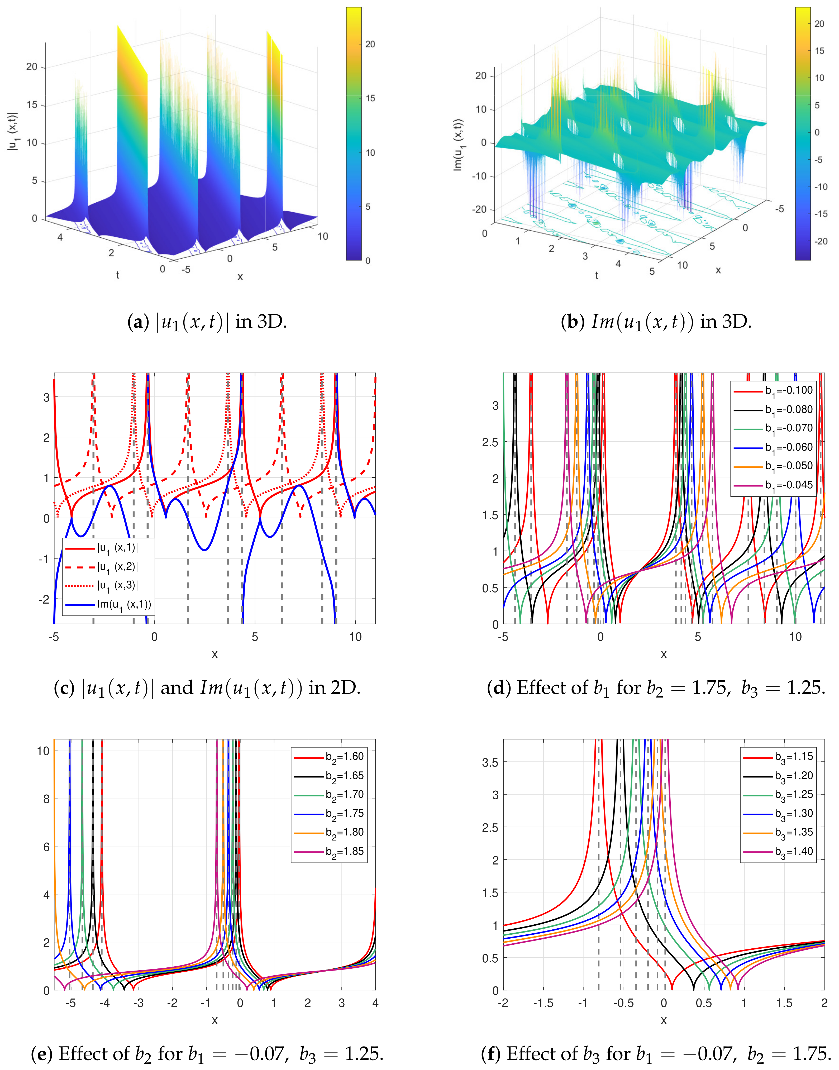
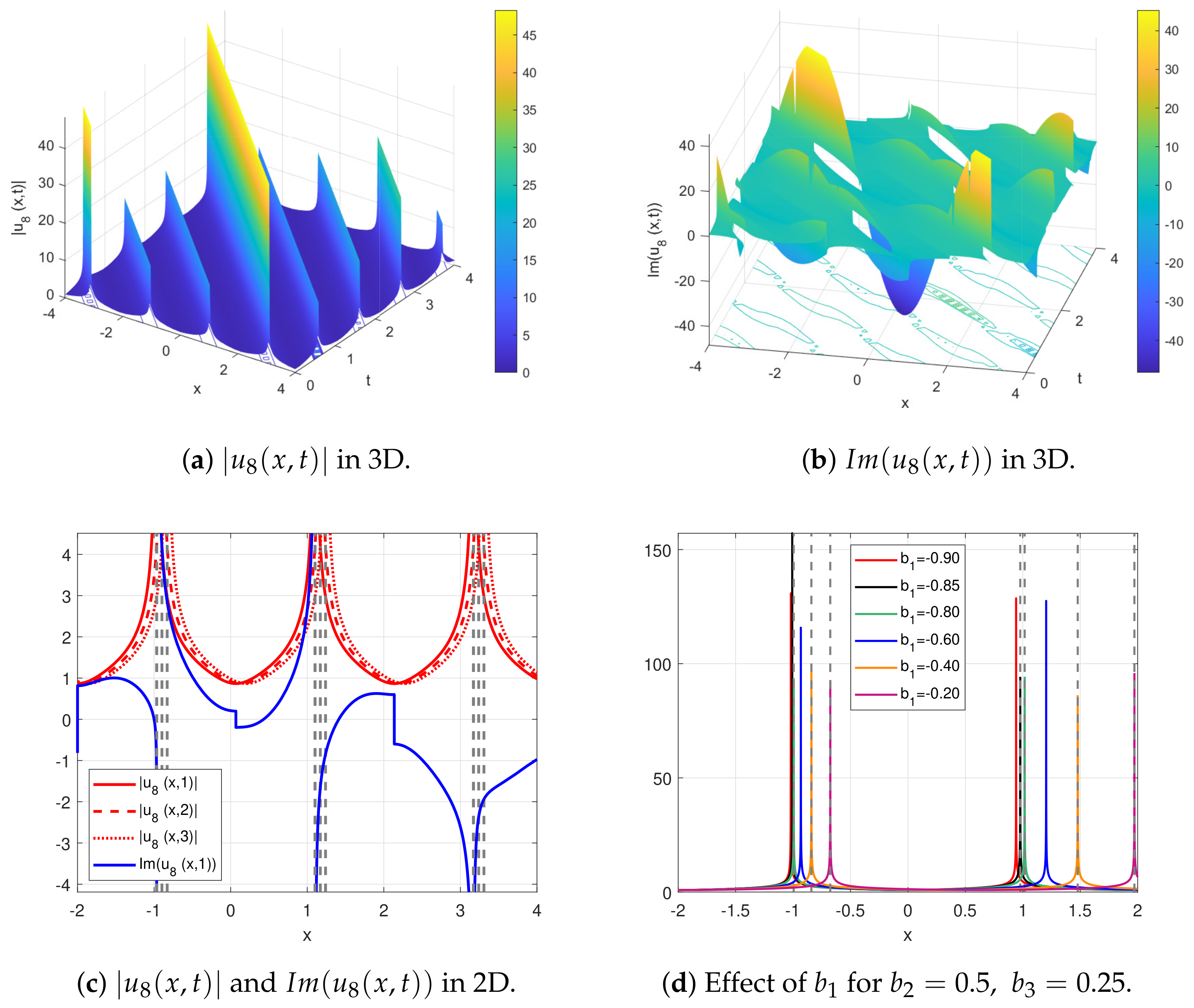
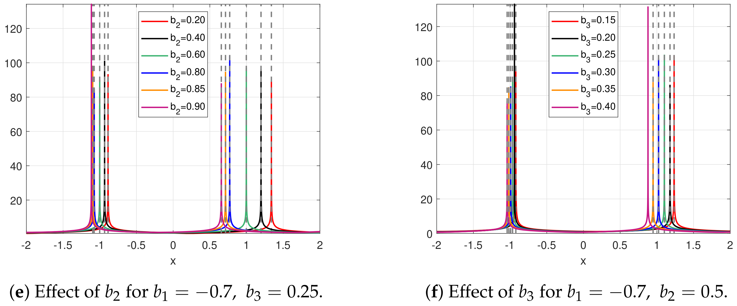
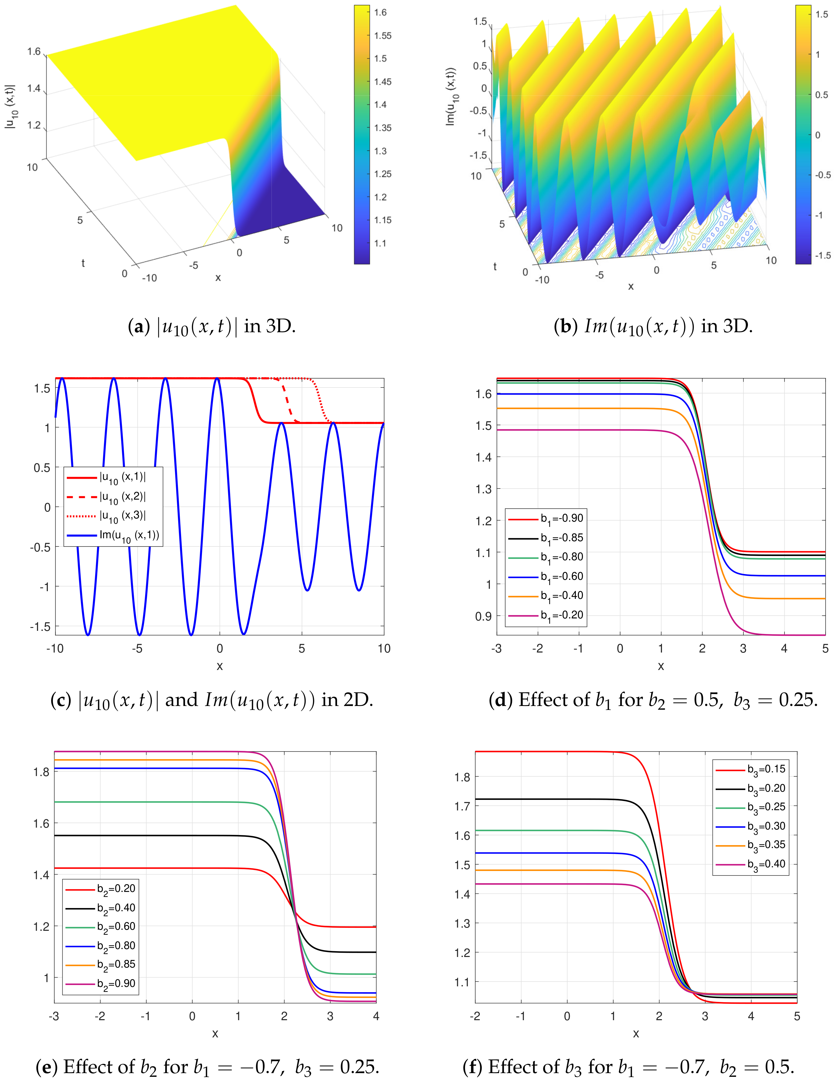
4. Results and Discussion

In this section, we depict some graphical representations of the obtained functions given in Equations (19)–(33) by using the sets in Equations (12)–(18). As we have emphasized before, our main goal is to obtain different types of soliton solutions and to see the effect of anti-cubic parameters on soliton behavior in each case. Each illustration consists of six sub-figures. They are (ia), (ib), (ic), (id), (ie) and (if) $(i,from1to7)$ and they represent the 3D of modulus, imaginary, 2D of modulus and imaginary together, the effect of $b_1$ in 2D, the effect of $b_2$ in 2D and the effect of $b_3$ in 2D, respectively.

Figure 1 depicts the some graphs of $u_1(x,t)$ in Equation (19) selecting the $Se{t}_1$ in Equation (12) with the assigned parameters values $h=-0.04,a=0.5,{\varphi }_0=0.5,$$b_1=-0.7,$$b_2=0.5,$$b_3=0.25,\kappa =2.$ From Figure 1a,c (red lines), it is possible to see the topological face of $\left|u_1(x,t)\right|$ and also the traveling wave properties which the soliton moves to the left depending on the times t = 1, 2, 3. Figure 1b,c (blue line) belong to $Im\left(u_1(x,t)\right).$ These graphs represent periodic behavior. Figure 1d–f are devoted to the effect of the anti-cubic parameter on the soliton behavior of $\left|u_1(x,t)\right|$ in Figure 1a. Figure d reflects the effect of $b_1$, which takes the values $-0.90,-0.85,-0.80,-0.60,-0.40$ and $-0.20$, respectively (colors from red to violet). Moreover, the other anti-cubic parameters take the values $b_2=0.5,b_3=0.25.$ Figure 1d, tells us that when $b_1$ takes the specified values and increases (red to violet), the soliton keeps its topological shape, there is no any movement on the horizontal axis, the peak of the soliton remains on the x-axis but the skirts of the soliton move vertically down. That is, $b_1$ causes the vertical amplitude of the soliton to decrease. At the same time, it is observed that there is an increase in the horizontal amplitude at the skirts of the soliton depending on the increase in the $b_1$ parameter (red to violet).

Figure 1e shows the effect of $b_2$ which takes the values 0.20, 0.40, 0.60, 0.80, 0.85 and 0.90, respectively (red to violet). Moreover, the other anti-cubic parameters take the values $b_1=-0.7,b_3=0.25.$ According to Figure 1e, the soliton also keeps its topological character, the skirts of the soliton remain on the horizontal axis, but depending on the increment in $b_2$, the peak of the soliton moves up vertically. At the same time, we can say that there is a relative increase in the horizontal amplitude of the soliton (red to violet). In other words, depending on the increase in $b_2$, the vertical amplitude of the soliton decreases and the soliton has a flatter appearance.

The effect of $b_3$ when taking the values 0.10, 0.20, 0.25, 0.30, 0.35 and 0.40, is depicted Figure 1f, considering the other anti-cubic parameters as $b_1=-0.7,b_2=0.5.$ It is seen that there is no movement on the horizontal axis, but depending on the increment in $b_3$, the skirts and peak of the soliton move down vertically. Furthermore, it is seen that there is a relative decrease in the horizontal amplitude of the soliton (red to violet). Therefore, it is observed that all three of the parameters $b_1$(Figure 1d,f), $b_2$ (Figure 1e) and $b_3$ (Figure 1f) have different and important effects on the topological soliton behavior of $\left|u_1(x,t)\right|$ in Figure 1a.

Figure 2 visualizes the peak soliton character and also the effect of the anti-cubic parameters on this soliton for the obtained optical soliton solution of $u_5(x,t)$ in Equation (23), with the $Se{t}_2$ in Equation (13) and the selected parameters $h=-0.04,a=-0.5,{\varphi }_0=0.5,$$b_1=-0.7,$$b_2=0.5,b_3=0.25,\kappa =2.$ It is observed from Figure 2a,c (red lines) that the soliton has the anti-peaked shape and travels to the right for the specific time t = 1, 2, 3. At the same time, there is a vertical amplitude (level) difference between the left and right skirts (wings) of the soliton. Figure 2b,c (blue line) belong to $Im\left(u_5(x,t)\right)$ and they reflect periodic solutions in different amplitudes. Figure 2d, depicts the effect of $b_1$ with the selected values $-0.90,-0.85,-0.80,-0.60,-0.40$ and −0.20, respectively (colors from red to violet), when $b_2=0.5,b_3=0.25.$ If we examine Figure 2d when $b_1$ takes the specified values and increases (red to violet), the soliton keeps its anti-peaked shape, moves to the right on the x-axis and the vertical amplitude of the soliton’s wings decreases. However, the skirts of the soliton move vertically down. That is, $b_1$ causes the vertical amplitude of the soliton to decrease. At the same time, it is observed that there is an increase in the horizontal amplitude at the skirts of the soliton depending on the increase in the $b_1$ parameter (red to violet). However, it should be noted that for the left wing of the soliton, this behavior is in the form of a decrease (increase) up to a certain value ($2<x_0\cong 2.136<2.5$). For the right wing, there is a decrease.

Figure 2e is the 2D projection of the effect of $b_2$ which takes the values 0.20, 0.40, 0.60, 0.80, 0.85 and 0.90, respectively (red to violet), when $b_1=-0.7,b_3=0.25.$ According to Figure 2e, the soliton also keeps its anti-peaked shape, the peak of the soliton remains on the horizontal axis, but depending on the increment in the $b_2$, the peak point of the soliton moves to the right and the vertical amplitude of the soliton also changes. This change is an increase in amplitude for the left wing of the soliton and a decrease for the right wing (red to violet).

Figure 2f belongs to $b_3$ which takes the values 0.15, 0.20, 0.25, 0.30, 0.35 and 0.40. The other anti-cubic parameters are $b_1=-0.7,b_2=0.5.$ Although Figure 2f is categorically similar to Figure 2e, it is clear that they do not express separate soliton behavior. Let us examine Figure 2f in a little more detail to see the difference. Depending on the increment in $b_3$, the soliton keeps its anti-peaked shape, the peak of the soliton remains on the x-axis but the soliton moves to the left, the amplitude of the left wing of the soliton decreases while the right wing’s amplitude increases. However, here we should also emphasize that for the right wing’s amplitude of the soliton, $\underset{x\to x_0>4}{lim}\left|u_5(x,1)\right|=1$ for all red to violet lines.

We illustrated some graphical representations of $u_1(x,t)$ in Equation (19) by using the $Se{t}_3$ in Equation (14) and with parameters $h=-0.04,a=-0.5,{\varphi }_0=0.5,b_1=-0.07,$$b_2=1.75,$$b_3=1.25,\kappa =2.$ Figure 3a,c generally reflect the periodic singular soliton character, but if the skirt parts of the soliton are taken into account, it is also possible to see the degenerated anti-cuspon character (color lines in Figure 3c). Additionally, we can name the soliton behavior of $Im\left(u_1(x,t)\right)$ as combination of cuspon and bright soliton (or anti-cuspon and dark) based on Figure 3b,c (blue lines).

If we examine Figure 3d, the soliton keeps its shape, the anti-peak point remains on the x-axis and the soliton travels to the left. Figure 3e is the graph that reflects the effect of $b_2$ on $\left|u_1(x,t)\right|$ in Figure 3a. According to Figure 3e, the peak point of the soliton shape takes an anti-cuspon character while the left and right wings of the soliton have a singular behavior. Additionally, the soliton moves to the left (red to violet). Figure 3f illustrates the effect of $b_3$ when it takes the values indicated on the graphs (red to violet). The soliton moves to the right and, depending on the increment in $b_3$, the soliton’s amplitude decreases (red to violet).

Figure 4 projects the different soliton behavior of the investigated equation. It is a depiction of $u_4(x,t)$ in Equation (22) with the selected $Se{t}_4$ in Equation (15) by assuming the parameter values as $h=-0.04,a=-0.5,{\varphi }_0=0.5,b_1=-0.7,b_2=0.5,b_3=0.25,\kappa =2.$ Consider Figure 4a,b (red lines) together. At first glance, these graphics reflect the singular-soliton character of $\left|u_4(x,t)\right|$. However, if one pays attention to the right part of the soliton, it will be seen that the anti-peaked-type soliton is present here, albeit with a small amplitude. Moreover, Figure 4c shows that the soliton has a traveling wave property and travels to the right at specific times t = 1, 2, 3. Figure 4b,c (blue line), which belong to $Im\left(u_4(x,t)\right)$, also reflect the singular soliton character. However, there are periodic fluctuations in the soliton on the left and right sides of the singular point. Figure 4d also visualizes in 2D the effect of $b_1$ with the assigned values $-0.90,-0.85,-0.80,-0.60,-0.40$ and −0.20, respectively. When $b_1$ increases from -0.90 to -0.20 (red to violet), the left wing and right wing of the soliton react differently. Please pay attention to the left wing. When $x_0<1.65$, the soliton’s amplitude increases but $1.65<x_s$ decreases ($x_s$ refers to a singular point for each case). From the right wing of the soliton, we see that amplitude of the soliton increases and the soliton travels to the right. Figure 4e also shows the effect of $b_2$ as in Figure 4d. However, this effect can be seen more clearly from Figure 4e. Figure 4f belongs to the effect of $b_3$ and also we see the same behavior in Figure 4d,e. Categorically, we cannot say that Figure 4f is the same as Figure 4e or d, because, if we examine the graph in Figure 4e in detail again, for the left part of the singular point, when $x_0<1.92$, the soliton’s amplitude decreases but $1.92<x_s$ increases ($x_s$ refers to a singular point for each case). The second difference is that, for the right part of the singular point, although the soliton’s amplitude decreases, the soliton moves to the left.

In Figure 5, we presented a different singular soliton shape of $u_8(x,t)$ in Equation (26) by using the $Se{t}_5$ in Equation (16) and the selected $h=0.04,a=0.5,{\varphi }_0=0.5,$$b_1=-0.7,$$b_2=0.5,b_3=0.25,\kappa =2.$

Figure 5a,c (red lines) portray the periodic singular shape of $\left|u_8(x,t)\right|$, while Figure 5b,c (blue line) reflect the strange singular shape.Figure 5d–f are the figures that show the effect of $b_1,b_2$ and $b_3$, respectively. Depending on the $b_i(i=1,2,3)$, in Figure 5d the soliton moves to the right, in Figure 5e,f the soliton moves to the left. As an even more important detail, the horizontal amplitude of the soliton increases when moving to the right (Figure 5d), and decreases when moving to the left (Figure 5e,f).

Considering the selected $Se{t}_6$ in Equation (17) and assigning the following special parameter values as $h=0.04,a=-0.5,{\varphi }_0=0.5,b_1=-0.07,b_2=-0.5,b_3=0.015,\kappa =2$, we depicted some illustrations $u_9(x,t)$ in Equation (27) by Figure 6. Although Figure 6a,c (red lines) seem to reflect the kink soliton behavior at first, upon a more careful examination, there is an anti-peaked soliton formed on the left bottom side, albeit with a very small amplitude for $\left|u_9(x,t)\right|$. Figure 6b,c (blue line) show the soliton profile of the $Im\left(u_9(x,t)\right)$ in 3D and 2D, respectively. The right part of both depictions propagates periodically while the left side fluctuates with smaller amplitude. Figure 6d, visualizes the effect of $b_1$ when taking the value given in the figure (red to violet). When $b_1$ takes the relevant values, the slope of the soliton, which determines the kink character, decreases. Although the right end of the soliton is seen to have the same amplitude values, the same effect is not seen on the left side. In addition, $b_1$ causes an increasing effect on the right wing of the soliton and a decreasing effect on the left wing of the soliton (red to violet colors), and the soliton moves to the left. Figure 6e,f also reflect the soliton character given by Figure 6a in a slightly more degenerate manner depending on the effect of $b_2$ and $b_3$, respectively. Although both graphs show that the soliton moves to the left, this effect is seen more clearly in Figure e.

Figure 7 is the graph obtained by the combination $u_{10}(x,t)$ in Equation (28), $Se{t}_7$ in Equation (18) and the parameters $h=0.04,a=-0.5,{\varphi }_0=0.5,b_1=-0.7,$$b_2=0.5,$$b_3=0.25,\kappa =2$, together. Figure 7a,c (red lines) are the 3D and 2D representations of $\left|u_{10}(x,t)\right|$ and showsthe kink soliton shape. Figure 7b,c (blue line) are the periodic waves in different amplitudes. Figure 7d belongs to effect of $b_1$ and reflects that the soliton remains in kink and moves down vertically, there is also a very small displacement to the left. The effect of $b_2$ is seen in Figure 7e, the vertical amplitude of the soliton changes depending on the increasing values of $b_2$, the solitons intersect at the value of $x_0\cong 2.25$, the soliton appears to move down (amplitude decreases) on the right of $x_0\cong 2.25$ and up (amplitude increases) on the left. A similar effect is observed for $b_3$ in Figure 7f, but on the left of $x_0\cong 2.77$ where the solitons intersect, the soliton appears to move down (amplitude decreases) and on the right of $x_0\cong 2.77$ the soliton moves up (amplitude increases).

5. Conclusions

In this article, many optical soliton solutions have been obtained by successfully examining the nonlinear Schrödinger equation having anti-cubic nonlinearity with the enhanced modified extended tanh expansion method. In this respect, the method yielded effective results. Various optical solitons have been derived, such as topological, anti-peaked, combined peaked-bright, combined anti-peaked dark, singular, combined singular anti-peaked, periodic singular, composite kink anti-peaked, kink, periodic and periodic with different amplitudes. Obtaining different types of solitons is one of the aims of the article, and the second goal, the effect of the parameters of the anti-cubic terms on soliton behavior, has been successfully investigated. The analysis was performed separately for each soliton obtained, and for the first time, the important results presented in this article were obtained, supported by graphics in the relevant section, and interpreted in detail. The obtained results show that the anti-cubic parameters have a significant effect on the soliton behavior of the NLSE-AC equation. This effect occurs differently depending on the type of the parameters, and the effect of the parameters also differs according to the soliton types. In addition, the parameter values used in the graphical representations are the parameter values determined as a result of long studies, and preserving the shape of the obtained soliton as the main goal. The most fundamental problem and difficulty at this point was the preservation of the delicate balance between the shape of the soliton and the anti-cubic parameters and even the anti-cubic parameters with each other. We believe that the results obtained in the article will be useful in a wide range of aspects, especially the behavior of solitons in optical fibers.

References

1. Arshad, M.; Seadawy, A.R.; Lu, D. Study of soliton solutions of higher-order nonlinear Schrödinger dynamical model with derivative non-Kerr nonlinear terms and modulation instability analysis. Results Phys. 2019, 13, 102305. [Google Scholar] [CrossRef]
2. Kudryashov, N.A. Stationary solitons of the model with nonlinear chromatic dispersion and arbitrary refractive index. Optik 2022, 259, 168888. [Google Scholar] [CrossRef]
3. Eldidamony, H.A.; Ahmed, H.M.; Zaghrout, A.S.; Ali, Y.S.; Arnous, A.H. Highly dispersive optical solitons and other solutions in birefringent fibers by using improved modified extended tanh-function method. Optik 2022, 256, 168722. [Google Scholar] [CrossRef]
4. Biswas, A.; Ekici, M.; Sonmezoglu, A.; Belic, M.R. Highly dispersive optical solitons with Kerr law nonlinearity by F-expansion. Optik 2019, 181, 1028–1038. [Google Scholar] [CrossRef]
5. Mirzazadeh, M.; Akinyemi, L.; Şenol, M.; Hosseini, K. A variety of solitons to the sixth-order dispersive (3+1)-dimensional nonlinear time-fractional Schrödinger equation with cubic-quintic-septic nonlinearities. Optik 2021, 241, 166318. [Google Scholar] [CrossRef]
6. Ozisik, M.; Cinar, M.; Secer, A.; Bayram, M. Optical solitons with Kudryashov’s sextic power-law nonlinearity. Optik 2022, 261, 169202. [Google Scholar] [CrossRef]
7. Kohl, R.W.; Biswas, A.; Ekici, M.; Zhou, Q.; Khan, S.; Alshomrani, A.S.; Belic, M.R. Highly dispersive optical soliton perturbation with cubic–quintic–septic refractive index by semi-inverse variational principle. Optik 2019, 199, 163322. [Google Scholar] [CrossRef]
8. Zayed, E.M.E.; Alngar, M.E.M.; Biswas, A.; Kara, A.H.; Ekici, M.; Alzahrani, A.K.; Belic, M.R. Cubic-quartic optical solitons and conservation laws with Kudryashov’s sextic power-law of refractive index. Optik 2021, 227, 166059. [Google Scholar] [CrossRef]
9. Biswas, A.; Ekici, M.; Sonmezoglu, A. Stationary optical solitons with Kudryashov’s quintuple power–law of refractive index having nonlinear chromatic dispersion. Phys. Lett. A 2022, 426, 127885. [Google Scholar] [CrossRef]
10. Kudryashov, N.A. Highly dispersive optical solitons of the equation with various polynomial nonlinearity law. Chaos Solitons Fractals 2020, 140, 110202. [Google Scholar] [CrossRef]
11. Triki, H.; Wazwaz, A.M. Soliton solutions of the cubic-quintic nonlinear Schrödinger equation with variable coefficients. Rom. J. Phys. 2016, 61, 360–366. [Google Scholar]
12. Al-Kalbani, K.K.; Al-Ghafri, K.S.; Krishnan, E.V.; Biswas, A. Pure-cubic optical solitons by Jacobi’s elliptic function approach. Optik 2021, 243, 167404. [Google Scholar] [CrossRef]
13. Rezazadeh, H.; Ullah, N.; Akinyemi, L.; Shah, A.; Mirhosseini-Alizamin, S.M.; Chu, Y.-M.; Ahmad, H. Optical soliton solutions of the generalized non-autonomous nonlinear Schrödinger equations by the new Kudryashov’s method. Results Phys. 2021, 24, 104179. [Google Scholar] [CrossRef]
14. Mirzazadeh, M.; Eslami, M.; Milovic, D.; Biswas, A. Topological solitons of resonant nonlinear Schrödinger equation with dual-power law nonlinearity by G/G-expansion technique. Optik 2014, 125, 5480–5489. [Google Scholar] [CrossRef]
15. Biswas, A.; Zhou, Q.; Moshokoa, S.P.; Triki, H.; Belic, M.; Alqahtani, R.T. Resonant 1-soliton solution in anti-cubic nonlinear medium with perturbations. Optik 2017, 145, 14–17. [Google Scholar] [CrossRef]
16. Asma, M.; Othman, W.A.M.; Wong, B.R.; Biswas, A. Optical soliton perturbation with quadratic-cubic nonlinearity by a semi-inverse variational principle. Proc. Rom. Acad. Ser. A Math. Phys. Tech. Sci. Inf. Sci. 2017, 18, 331–336. [Google Scholar]
17. Fedele, R.; Schamel, H.; Karpman, V.I.; Shukla, P.K. Envelope solitons of nonlinear Schrödinger equation with an anti-cubic nonlinearity. J. Phys. A Math. Gen. 2003, 36, 1169. [Google Scholar] [CrossRef] [Green Version]
18. Biswas, A.; Ekici, M.; Sonmezoglu, A.; Belic, M. Chirped and chirp-free optical solitons with generalized anti-cubic nonlinearity by extended trial function scheme. Optik 2019, 178, 636–644. [Google Scholar] [CrossRef]
19. Krishnan, E.V.; Biswas, A.; Zhou, Q.; Babatin, M.M. Optical solitons with anti-cubic nonlinearity by mapping methods. Optik 2018, 170, 520–526. [Google Scholar] [CrossRef]
20. Jawad, A.J.M.; Mirzazadeh, M.; Zhou, Q.; Biswas, A. Optical solitons with anti-cubic nonlinearity using three integration schemes. Superlattices Microstruct. 2017, 105, 1–10. [Google Scholar] [CrossRef] [Green Version]
21. Wafaa, R.B.; Ahmed, H.M.; Seadawy, A.R.; Althobaiti, A. The higher-order nonlinear Schrödinger’s dynamical equation with fourth-order dispersion and cubic-quintic nonlinearity via dispersive analytical soliton wave solutions. Opt. Quantum Electron. 2021, 53, 668. [Google Scholar]
22. Triki, H.; Kara, A.H.; Biswas, A.; Moshokoa, S.P.; Belic, M. Optical solitons and conservation laws with anti-cubic nonlinearity. Optik 2016, 127, 12056–12062. [Google Scholar] [CrossRef]
23. Muniyappan, A.; Hemamalini, D.; Akila, E.; Elakkiya, V.; Anitha, S.; Devadharshini, S.; Biswas, A.; Yıldırım, Y.; Alshehri, H.M. Bright solitons with anti-cubic and generalized anti-cubic nonlinearities in an optical fiber. Optik 2022, 254, 168612. [Google Scholar] [CrossRef]
24. Ekici, M.; Mirzazadeh, M.; Sonmezoglu, A.; Ullah, M.Z.; Zhou, Q.; Triki, H.; Moshokoa, S.P.; Biswas, A. Optical solitons with anti-cubic nonlinearity by extended trial equation method. Optik 2017, 136, 368–373. [Google Scholar] [CrossRef]
25. Biswas, A. Conservation laws for optical solitons with anti-cubic and generalized anti-cubic nonlinearities. Optik 2019, 176, 198–201. [Google Scholar] [CrossRef]
26. Foroutan, M.; Manafian, J.; Ranjbaran, A. Solitons in optical metamaterials with anti-cubic law of nonlinearity by generalized G/G-expansion method. Optik 2018, 162, 86–94. [Google Scholar] [CrossRef]
27. Foroutan, M.; Manafian, J.; Ranjbaran, A. Solitons in optical metamaterials with anti-cubic law of nonlinearity by ETEM and IGEM. J. Eur. Opt.-Soc.-Rapid Publ. 2018, 14, 16. [Google Scholar] [CrossRef] [Green Version]
28. Kudryashov, N.A. Exact solutions of equation for description of embedded solitons. Optik 2022, 268, 169801. [Google Scholar] [CrossRef]
29. Kudryashov, N.A. Solitary waves of model with triple arbitrary power and non-local nonlinearity. Optik 2022, 262, 169334. [Google Scholar] [CrossRef]
30. Kudryashov, N.A. Optical solitons of the model with generalized anti-cubic nonlinearity. Optik 2022, 257, 168746. [Google Scholar] [CrossRef]
31. Kudryashov, N.A. Bright and dark solitons in a nonlinear saturable medium. Phys. Lett. A 2022, 427, 127913. [Google Scholar] [CrossRef]
32. Kudryashov, N.A.; Lavrova, S.F. Dynamical properties of the generalized model for description of propagation pulses in optical fiber with arbitrary refractive index. Optik 2021, 245, 167679. [Google Scholar] [CrossRef]
33. Kudryashov, N.A.; Safonova, D.V. Painleve analysis and traveling wave solutions of the sixth order differential equation with non-local nonlinearity. Optik 2021, 244, 167586. [Google Scholar] [CrossRef]
34. Kudryashov, N.A. The Lakshmanan-Porsezian-Daniel model with arbitrary refractive index and its solution. Optik 2021, 241, 167043. [Google Scholar] [CrossRef]
35. Yildirim, Y. Optical solitons to Kundu-Mukherjee-Naskar model with trial equation approach. Optik 2019, 183, 1061–1065. [Google Scholar] [CrossRef]
36. Yildirim, Y. Optical solitons to Biswas-Arshed model in birefringent fibers using modified simple equation architecture. Optik 2019, 182, 1149–1162. [Google Scholar] [CrossRef]
37. Yildirim, Y. Optical solitons to Chen-Lee-Liu model in birefringent fibers with trial equation approach. Optik 2019, 183, 881–886. [Google Scholar] [CrossRef]
38. Yildirim, Y. Sub pico-second pulses in mono-mode optical fibers with Triki- Biswas model using trial equation architecture. Optik 2019, 183, 463–466. [Google Scholar] [CrossRef]
39. Yildirim, Y. Optical solitons to Sasa-Satsuma model in birefringent fibers with modified simple equation approach. Optik 2019, 184, 197–204. [Google Scholar] [CrossRef]
40. Yildirim, Y. Optical solitons to Sasa-Satsuma model with trial equation approach. Optik 2019, 184, 70–74. [Google Scholar] [CrossRef]
41. Yildirim, Y. Optical solitons to Kundu-Mukherjee-Naskar model in birefringent fibers with trial equation approach. Optik 2019, 183, 1026–1031. [Google Scholar] [CrossRef]
42. Yildirim, Y. Optical solitons to Schrödinger-Hirota equation in DWDM system with trial equation integration architecture. Optik 2019, 182, 275–281. [Google Scholar] [CrossRef]
43. Yildirim, Y. Optical solitons of Biswas-Arshed equation by trial equation technique. Optik 2019, 182, 876–883. [Google Scholar] [CrossRef]
44. Yildirim, Y. Optical solitons to Gerdjikov-Ivanov equation in birefringent fibers with trial equation integration architecture. Optik 2019, 182, 349–355. [Google Scholar] [CrossRef]
45. Yildirim, Y. Optical solitons of Gerdjikov-Ivanov equation with four-wave mixing terms in birefringent fibers by modified simple equation methodology. Optik 2019, 182, 745–754. [Google Scholar] [CrossRef]
46. Yildirim, Y. Optical solitons of Gerdjikov-Ivanov equation in birefringent fibers with modified simple equation scheme. Optik 2019, 182, 424–432. [Google Scholar] [CrossRef]
47. Yildirim, Y. Optical solitons of Biswas-Arshed equation in birefringent fibers by trial equation technique. Optik 2019, 182, 810–820. [Google Scholar] [CrossRef]
48. Yildirim, Y. Optical solitons in DWDM technology with four-wave mixing by trial equation integration architecture. Optik 2019, 182, 625–632. [Google Scholar] [CrossRef]
49. Yildirim, Y. Bright, dark and singular optical solitons to Kundu-Eckhaus equation having four-wave mixing in the context of birefringent fibers by using of trial equation methodology. Optik 2019, 182, 393–399. [Google Scholar] [CrossRef]
50. Yildirim, Y. Optical solitons of Biswas-Arshed equation by modified simple equation technique. Optik 2019, 182, 986–994. [Google Scholar] [CrossRef]
Figure 1. The various illustrations of u 1 ( x , t ) in Equation (19) by combination of the S e t 1 in Equation (12) and the selected h = 0.04 , a = 0.5 , ϕ 0 = 0.5 , b 1 = 0.7 , b 2 = 0.5 , b 3 = 0.25 , κ = 2 values.
Mathematics 11 01215 g001aMathematics 11 01215 g001b
Figure 2. The various views of u 5 ( x , t ) in Equation (23) by combination of the S e t 2 in Equation (13) and the selected h = 0.04 , a = 0.5 , ϕ 0 = 0.5 , b 1 = 0.7 , b 2 = 0.5 , b 3 = 0.25 , κ = 2 values.
Mathematics 11 01215 g002
Figure 3. The various depictions of u 1 ( x , t ) in Equation (19) by combination of the S e t 3 in Equation (14) and the selected h = 0.04 , a = 0.5 , ϕ 0 = 0.5 , b 1 = 0.07 , b 2 = 1.75 , b 3 = 1.25 , κ = 2 values.
Mathematics 11 01215 g003
Figure 4. The various projections of u 4 ( x , t ) in Equation (22) by combination of the S e t 4 in Equation (15) and the selected h = 0.04 , a = 0.5 , ϕ 0 = 0.5 , b 1 = 0.7 , b 2 = 0.5 , b 3 = 0.25 , κ = 2 values.
Mathematics 11 01215 g004aMathematics 11 01215 g004b
Figure 5. The various simulations of u 8 ( x , t ) in Equation (26) by combination of the S e t 5 in Equation (16) and the selected h = 0.04 , a = 0.5 , ϕ 0 = 0.5 , b 1 = 0.7 , b 2 = 0.5 , b 3 = 0.25 , κ = 2 values.
Mathematics 11 01215 g005aMathematics 11 01215 g005b
Figure 6. The various portraits of u 9 ( x , t ) in Equation (27) by combination of the S e t 6 in Equation (17) and the selected h = 0.04 , a = 0.5 , ϕ 0 = 0.5 , b 1 = 0.07 , b 2 = 0.5 , b 3 = 0.015 , κ = 2 values.
Mathematics 11 01215 g006aMathematics 11 01215 g006b
Figure 7. The various silhouettes of u 10 ( x , t ) in Equation (28) by combination of the S e t 7 in Equation (18) and the selected h = 0.04 , a = 0.5 , ϕ 0 = 0.5 , b 1 = 0.7 , b 2 = 0.5 , b 3 = 0.25 , κ = 2 values.
Mathematics 11 01215 g007