Ensemble Methods in Customer Churn Prediction: A Comparative Analysis of the State-of-the-Art

Abstract

In the past several single classifiers, homogeneous and heterogeneous ensembles have been proposed to detect the customers who are most likely to churn. Despite the popularity and accuracy of heterogeneous ensembles in various domains, customer churn prediction models have not yet been picked up. Moreover, there are other developments in the performance evaluation and model comparison level that have not been introduced in a systematic way. Therefore, the aim of this study is to perform a large scale benchmark study in customer churn prediction implementing these novel methods. To do so, we benchmark 33 classifiers, including 6 single classifiers, 14 homogeneous, and 13 heterogeneous ensembles across 11 datasets. Our findings indicate that heterogeneous ensembles are consistently ranked higher than homogeneous ensembles and single classifiers. It is observed that a heterogeneous ensemble with simulated annealing classifier selection is ranked the highest in terms of AUC and expected maximum profits. For accuracy, F1 measure and top-decile lift, a heterogenous ensemble optimized by non-negative binomial likelihood, and a stacked heterogeneous ensemble are, respectively, the top ranked classifiers. Our study contributes to the literature by being the first to include such an extensive set of classifiers, performance metrics, and statistical tests in a benchmark study of customer churn.

1. Introduction

Customer retention has proven to be valuable for a company in several ways [1]. First, customer retention will make sure that companies can focus on keeping their existing customers happy instead of attracting new risky customers. Second, satisfied customers spread positive word-of-mouth and thereby attracting potential leads. The same holds for dissatisfied customers who can share negative experiences, meaning that it is vital to keep customers happy. Third, long-term customers are also more loyal and less costly to serve given the knowledge of their previous demands. Finally, it is around five or six times cheaper to retain customers than to acquire them. Hence, successful customer retention does not only reduce costs but can also induce an increase in profit [2].

Because of the significant financial implications of correctly predicting customer churn [1,2], customer churn prediction (CCP) models have become utterly important in customer relationship management (CRM) to identify the customers who are most likely to terminate their relationship [3]. As a result, there has been a lot of focus on developing new methods to improve the accuracy of the churn predictions [2]. Traditionally, CCP models are divided into single classifiers and ensembles. Among the plethora of single classifiers, logistic regression and decision trees are the two most popular techniques because of their simplicity, interpretability, and reasonable performance [4,5]. Other important single classifiers for predicting churn are naive Bayes, support vector machines, and neural networks [6].

Besides single classifiers, ensembles such as random forest and adaboost have proven to yield superior performance compared to single classifiers in various studies [7,8]. There are two kinds of ensembles, namely, homogeneous and heterogeneous [9]. Homogeneous ensembles combine the same base classifier using different sampling methods [10,11]. Heterogenous ensembles are a combination of different base classifiers, which can be single classifiers but also homogeneous ensembles.

Despite the fact that there are two kinds of ensembles, homogeneous ensembles have been getting the most attention in CCP literature. This is a missed opportunity since large scale benchmark studies in related domains have proven the value of heterogeneous ensembles [9,12]. Given the comparative little attention to heterogeneous ensembles in CCP, several design issues remain unclear. Besides the inclusion of heterogenous ensembles in the set of classifiers, there are several other recent advances in predictive analytics that have received little attention in large scale CCP benchmark studies, namely, (1) the introduction of highly competitive methods such as the logit leaf [13], lightGBM [14], and catboost [15]; (2) the different type of performance metrics including profit-based model evaluation [16]; and (3) the use of both statistical and Bayesian hypothesis testing to compare classifier performance [17].

Our contributions are the following:

• We provide a comprehensive overview of the state-of-the-art ensemble methods in CCP and conduct the largest benchmark study to date. More specifically, we compare 6 single classifiers, 14 homogeneous ensembles, and 13 heterogeneous ensembles across 11 public and private data sets. By using several open-source data sets we ensure that our results are replicable and generalizable.
• We include several novel classifiers that have not yet been included in large scale benchmark studies. Especially, gradient boosting implementations such as lightGBM and catboost have received comparatively little attention in CCP. However, these models have empirically demonstrated to outperform other classifiers in other domains (e.g., [18,19]).
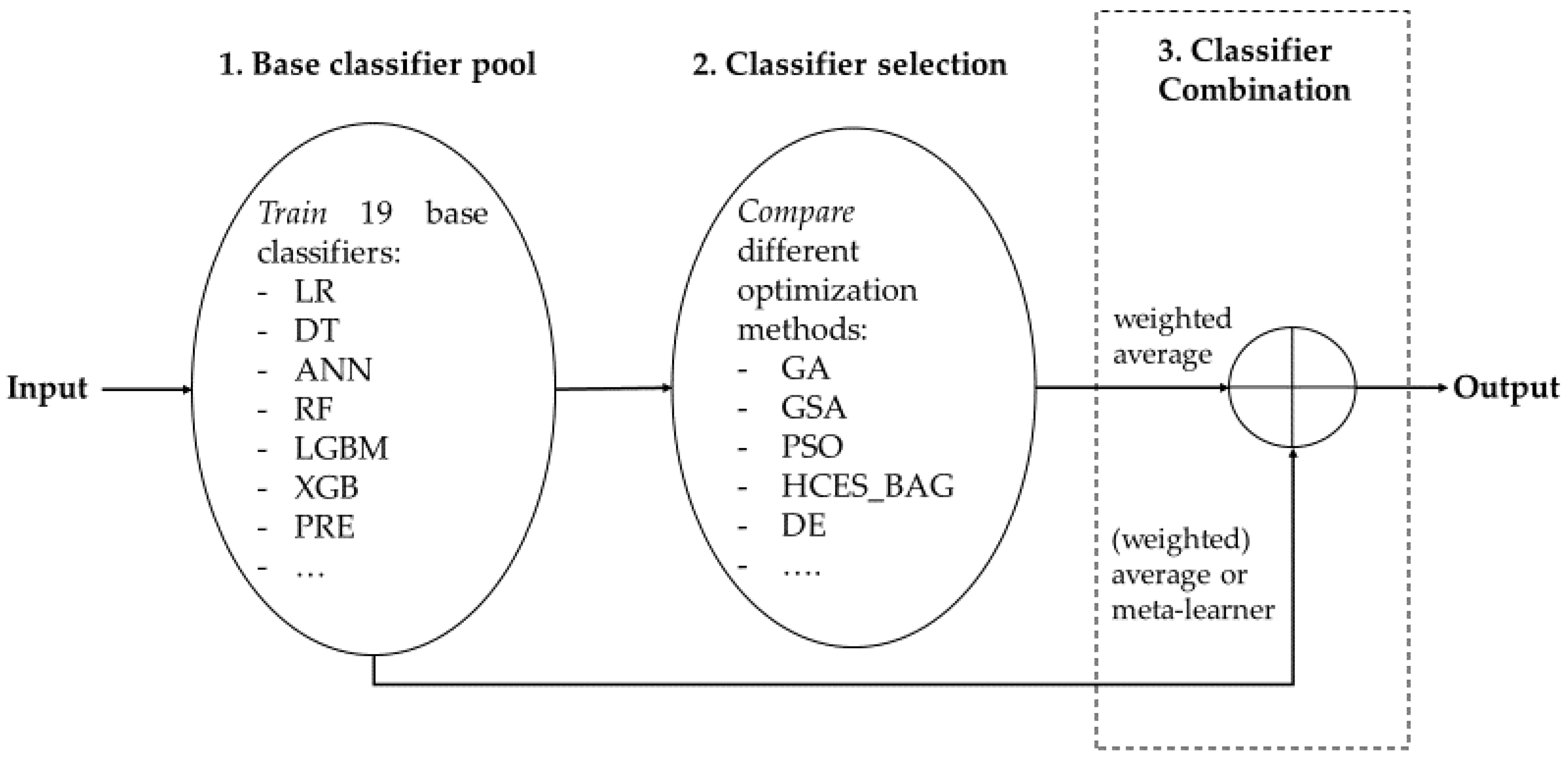
• We develop novel heterogeneous ensembles using a wide variety of base classifiers and advanced classifier selection methods that have not been used in previous work. For the base classifier pool, we apply several powerful classifiers into the heterogeneous ensemble framework [20]. For the classifier selection methods, research has mainly adopted heuristic search procedures such as hill climbing [21]. To the best of our knowledge, we are the first to compare advanced meta-heuristic and statistical optimization procedures to perform classifier selection.
• We use five different types of evaluation metrics that each measure a different aspect of CCP model performance, namely, overall statistical performance, performance for top ranked would-be churners, and profit-driven performance.
• Both frequentist and Bayesian hypothesis tests are applied to test the significance of our results. More specifically, the Friedman test with the Rom’s procedure [22] and the Bayesian signed-rank test with region of practical significance (ROPE) are performed [23].

The remaining paper is structured as follows. We start by discussing prior research in CCP. Next, we present the different classifiers and go over the experimental set-up. Finally, we present the results and give our definitive conclusion and recommendations for future research.

2. Related Work

2.1. Ensemble Methods

Ensemble methods are a popular way to increase the predictive accuracy of single classifiers. Ensemble methods are often referred to as multi-classifier systems since they combine the strengths of multiple classifiers to achieve better performance than the best individual classifier [24]. From a theoretical point-of-view, ensemble methods solve the statistical, computational, and representational problems associated with single classifiers [25]. In essence, these theories state that multiple classifiers filter out faulty hypotheses, overcome local optima, and cover different parts of the input space, thereby complementing each other’s deficiencies and increasing predictive performance [24]. Research has concluded that the performance of ensemble methods are driven by diversity and accuracy [26]. Diversity means that the constituent members of an ensemble should reach different decisions to increase performance. Ideally, an ensemble strives for high accuracy of the individual members combined with high level of disagreement between the members.

Creating an ensemble method includes two steps: determining the base classifiers and combining the outputs of the individual base classifiers [9]. Homogeneous ensembles pool together predictions of the same base classifier to achieve better predictions [9]. The main idea behind homogeneous ensembles is to create differences among the individual members by promoting data-driven diversity. Data-driven diversity can be created by partitioning the data or feature space such that it is different for each model [26]. The most well-known data-driven diversity generators are bagging, random subspaces, boosting, and rotation forest [9]. Since the constituent members of the ensemble should be sensitive to small changes, decision trees are among the most popular base classifiers.

Heterogeneous ensembles combine different base classifiers and add another step to the ensemble creation process, namely, classifier selection or classifier pruning [11]. After creating the initial base classifier pool, heterogeneous ensembles intelligently select the optimal set of classifiers before combining their outputs. Classifier selection can thus be tackled as an optimization problem with the objective of reaching maximum accuracy (or any other performance metric). By doing so, heterogeneous ensembles promote both high accuracy (i.e., only highly performant members enter the ensemble) and diversity (i.e., different base classifiers cover different parts of the solution space). The included base classifiers can be either single classifiers or homogeneous ensembles [25]. Since theory states that ensembles are likely to perform better than the individual quality of the best possible constituent member, heterogeneous ensembles should theoretically outperform homogeneous ensembles.

In sum, the difference between homogeneous and heterogeneous ensembles are twofold. First, the base classifiers in homogeneous ensembles are always the same single classifiers, and diversity is created via variations in the input data or features. Heterogenous ensembles start from a pool of different classifiers and create diversity via variations in classifiers and input data. Second, homogenous ensembles give an equal weight to the results of each base classifier by simply combining the responses of each individual model. Heterogeneous ensembles intelligently select which classifiers to include in the final ensemble and attribute a higher weight to more performant members in the final combination.

2.2. Ensemble Methods in Customer Churn

Customer churn prediction is a procedure to allocate a probability to churn to a customer based on the relationship between historical data and future tendencies [27]. Customer churn prediction can be considered as a binary classification problem in which the performance depends on the quality of the historical data and the chosen classifier [28]. Previous research has shown that there is a direct link between the chosen classifier and the return on investment of a retention campaign [2,5]. As a result, several single classifiers, homogenous and heterogeneous ensembles, have been proposed to accurately predict customer churn.

Table 1 summarizes research on customer churn prediction literature based upon the used classifiers, performance metrics, and statistical tests. To include all relevant articles, we searched in the major journal databases, such as Elsevier, IEEE Xplore, SpringerLink, ScienceDirect, ACM Digital Library, and Google Scholar. In these databases, the search term criteria were based on the following terms: {‘customer churn’ or ‘customer attrition’ or ‘customer retention’, or ‘churn’} and {‘ensemble’}. The main criteria to include papers were: (1) articles containing the search terms in the keywords or abstract or title; (2) articles published in journals, conference proceedings, or lecture notes; (3) articles published between 2005 and 2022 with a special emphasis on the last 5 years; (4) the inclusion of at least one ensemble method; and (5) performing an empirical comparison of different classifiers. Articles that do not use an ensemble method were immediately discarded. The goal of the literature review was not to provide a complete overview of customer churn prediction. For a general overview of customer churn prediction, we refer the reader to [1,2,3].

Classifiers in CCP are categorized into single classifiers, homogenous and heterogeneous ensembles. Research using single classifiers often includes models such as logistic regression [29], decision trees [30], support vector machines [31], and neural networks [32]. Although logistic regression is often seen as the gold standard, other studies have demonstrated that other techniques are capable of performing better [13]. For example, Vafeiadis et al. [6] showed that logistic regression underperformed when compared to neural networks, decision trees, and support vector machine classifiers. To increase the performance of single classifiers, a wide range of homogeneous and heterogenous ensembles have been proposed. For example, Coussement et al. [7] shows that decision trees and generalized additive models underperform when compared to their ensemble counterparts, random forest, and generalized additive model ensembles. Baumann et al. [33] showed that a selective hill climbing heterogenous ensemble outperformed all other single classifiers and homogeneous ensembles.

Evaluation metrics in CCP are classified according to whether they are cut-off dependent, cut-off independent, or take profits into account. In the case of cut-off dependent measures, a threshold should be set to determine whether or not a customer is classified as a churner. After the cut-off is chosen, several metrics are calculated based on the confusion matrix. The most popular cut-off dependent metrics in CCP are accuracy and top-decile lift [2]. Cut-off independent measures, on the other hand, are independent of the chosen threshold and the operating conditions [34]. The Area under the Receiver Operating Characteristic (AUC) is the most well-known metric since it intuitively estimates the probability that a randomly chosen churner is ranked higher than a non-churner [31]. Finally, profit-driven performance metrics take into account the expected profits of setting up a targeted advertising campaign [35]. The expected maximum profit criterion for churn (EMPC) incorporates the costs and benefits of a retention campaign into a coherent performance measure and allows to select the most profitable customers [16].

Finally, CCP studies are characterized by whether or not they use a formal testing procedure to compare the results. There are two types of procedures, namely, statistical or Bayesian tests. The former methods range from pairwise to non-pairwise and parametric and non-parametric tests [22,36]. Among the plethora of statistical testing procedures, the non-parametric Friedman test with family-wise error correction is the most popular [13]. Several Bayesian alternatives are available to their frequentist counterparts but have not yet found their introduction in CCP.

Looking at Table 1, several trends can be spotted. First, future studies will continue to look for the silver bullet and introduce novel highly accurate ensemble method. This can be achieved by introducing highly performant models in the base classifier pool [37] or employing general purpose solvers with specific objective function for tuning which the individual models enter the ensemble [9]. Another stream of research will further focus on designing ensembles which directly maximize the business objective, with an emphasis on profit-centered optimization [21]. A final trend is the search for both accurate and interpretable ensemble models and coming up with methods to open the black box [38].

Table 1. Overview of ensemble methods in customer churn prediction.

	Classifiers 1				Evaluation 2				Tests 3
Study	Single	Hm	Ht	No 4	D	I	P	No	Stat	B
Buckinx and Van den Poel 2005 [39]	X	X		3	X	X		2
Lemmens and Croux 2006 [8]	X	X		4	X	X		3
Burez and Van den Poel 2007 [29]	X	X		3	X	X	X	3
Coussement and Van den Poel 2008 [40]	X	X		3	X	X		3	X
Burez and Van den Poel 2009 [41]	X	X		2	X	X		3	X
Tsai and Lu 2009 [32]	X		X	3	X			3	X
Xie et al., 2009 [42]		X		4	X			2
De Bock and Van den Poel 2011 [43]		X		5	X	X		4	X
Ballings and Van den Poel 2012 [4]	X	X		3		X		1	X
De Bock and Van den Poel 2012 [44]	X	X		6	X	X		4	X
Kim et al., 2012 [45]	X	X		6	X			1
Verbeke et al., 2012 [2]	X	X		16	X	X	X	3	X
Coussement and De Bock 2013 [7]	X	X		4	X			2	X
Idriss et al., 2012 [46]	X	X		5		X		4
Baumann et al., 2015 [33]	X		X	15	X			1	X
Vafeiadis et al., 2015 [6]	X	X		6	X			4
Coussement et al., 2017 [27]	X	X		9	X	X		2	X
Idriss and Khan 2017 [47]	X	X	X	5	X	X		2
Oskarsdottir et al., 2017 [35]	X	X		3	X	X	X	4	X
Zhu et al., 2018 [48]		X		3			X	1	X
Zhu et al., 2017 [49]	X	X	X	7	X	X	X	3	X
De Caigny et al., 2018 [13]	X	X		5	X	X		2	X
Zhu et al., 2018 [50]	X	X		4	X	X	X	3	X
Ullah et al., 2019 [10]	X	X		11	X	X		6
Jain et al., 2020 [51]	X	X		2	X	X		8
Bhujbal and Bavdane 2021 [52]	X	X	X	7	X			1
Chowdhury et al., 2021 [53]		X		4	X	X		2
Deng et al., 2021 [54]		X		3	X	X		3
De Bock and De Caigny 2021 [38]	X	X		8	X	X		2	X
Janssens et al., 2022 [55]	X	X		7	X	X	X	3	X
Karuppaiah and Palanisamy 2021 [56]	X	X	X	5	X	X		2
Kiguchi et al., 2022 [57]	X	X		3	X	X		2
Lessmann et al., 2021 [21]	X	X	X	18	X	X	X	3	X
Sagala and Permai 2021 [58]		X		3	X	X		2
Vo et al., 2021 [59]	X	X		4	X			4	X
Wu et al., 2021 [11]	X	X		6	X	X		5
Gattermann and Thonemann 2021 [60]	X	X		3	X	X		2
Mirkovic et al., 2022 [28]	X	X		3	X	X		2
Our study	X	X	X	33	X	X	X	5	X	X

¹ The abbreviations stand for: single = single classifiers, Hm = homogeneous ensemble, Ht = heterogeneous ensemble, No = number of classifiers. ² The abbreviations stand for: D = cut-off dependent measures, I = cut-off independent measures, P = profit-driven measures, No = number of evaluation metrics. ³ The abbreviations stand for: Stat = statistical hypothesis testing, B = Bayesian testing. ⁴ We only count the number of unique classifiers (No). For example, if a support vector machine is used with a linear and a polynomial kernel this is only counted as one classifier.

Table 1. Overview of ensemble methods in customer churn prediction.

	Classifiers 1				Evaluation 2				Tests 3
Study	Single	Hm	Ht	No 4	D	I	P	No	Stat	B
Buckinx and Van den Poel 2005 [39]	X	X		3	X	X		2
Lemmens and Croux 2006 [8]	X	X		4	X	X		3
Burez and Van den Poel 2007 [29]	X	X		3	X	X	X	3
Coussement and Van den Poel 2008 [40]	X	X		3	X	X		3	X
Burez and Van den Poel 2009 [41]	X	X		2	X	X		3	X
Tsai and Lu 2009 [32]	X		X	3	X			3	X
Xie et al., 2009 [42]		X		4	X			2
De Bock and Van den Poel 2011 [43]		X		5	X	X		4	X
Ballings and Van den Poel 2012 [4]	X	X		3		X		1	X
De Bock and Van den Poel 2012 [44]	X	X		6	X	X		4	X
Kim et al., 2012 [45]	X	X		6	X			1
Verbeke et al., 2012 [2]	X	X		16	X	X	X	3	X
Coussement and De Bock 2013 [7]	X	X		4	X			2	X
Idriss et al., 2012 [46]	X	X		5		X		4
Baumann et al., 2015 [33]	X		X	15	X			1	X
Vafeiadis et al., 2015 [6]	X	X		6	X			4
Coussement et al., 2017 [27]	X	X		9	X	X		2	X
Idriss and Khan 2017 [47]	X	X	X	5	X	X		2
Oskarsdottir et al., 2017 [35]	X	X		3	X	X	X	4	X
Zhu et al., 2018 [48]		X		3			X	1	X
Zhu et al., 2017 [49]	X	X	X	7	X	X	X	3	X
De Caigny et al., 2018 [13]	X	X		5	X	X		2	X
Zhu et al., 2018 [50]	X	X		4	X	X	X	3	X
Ullah et al., 2019 [10]	X	X		11	X	X		6
Jain et al., 2020 [51]	X	X		2	X	X		8
Bhujbal and Bavdane 2021 [52]	X	X	X	7	X			1
Chowdhury et al., 2021 [53]		X		4	X	X		2
Deng et al., 2021 [54]		X		3	X	X		3
De Bock and De Caigny 2021 [38]	X	X		8	X	X		2	X
Janssens et al., 2022 [55]	X	X		7	X	X	X	3	X
Karuppaiah and Palanisamy 2021 [56]	X	X	X	5	X	X		2
Kiguchi et al., 2022 [57]	X	X		3	X	X		2
Lessmann et al., 2021 [21]	X	X	X	18	X	X	X	3	X
Sagala and Permai 2021 [58]		X		3	X	X		2
Vo et al., 2021 [59]	X	X		4	X			4	X
Wu et al., 2021 [11]	X	X		6	X	X		5
Gattermann and Thonemann 2021 [60]	X	X		3	X	X		2
Mirkovic et al., 2022 [28]	X	X		3	X	X		2
Our study	X	X	X	33	X	X	X	5	X	X

¹ The abbreviations stand for: single = single classifiers, Hm = homogeneous ensemble, Ht = heterogeneous ensemble, No = number of classifiers. ² The abbreviations stand for: D = cut-off dependent measures, I = cut-off independent measures, P = profit-driven measures, No = number of evaluation metrics. ³ The abbreviations stand for: Stat = statistical hypothesis testing, B = Bayesian testing. ⁴ We only count the number of unique classifiers (No). For example, if a support vector machine is used with a linear and a polynomial kernel this is only counted as one classifier.

2.3. Conclusions of the Related Work

From Table 1, the following conclusions can be drawn. First, the performance of ensembles is often compared to single classifiers. In several studies, logistic regression is considered as the gold standard, and novel approaches are designed to outperform the benchmark [31]. Whereas this approach can be beneficial to check whether a simple solution is not better, novel methods should ideally be benchmarked against other ensemble models. Moreover, the average number of classifiers is equal to 5.70, which is rather low for a large scale benchmark study. The reason for this low number can be found in the fact that most researchers make an intelligent selection of classifiers to compare to their novel method [13] or adapt the selected algorithms to their business setting [11].

Second, homogeneous ensembles are very common and are examined in almost every study. This is probably due to their overall good performance and the ease of constructing such models because of the off-the-shelf implementations available in business analytics software such as Microsoft Azure Machine Learning, IBM Watson, Google Cloud AI, etc., and open source programming languages such as R, Python, Julia, Java, and many others.

Third, only four studies have investigated the use of heterogeneous ensembles, also referred to as selective ensembles. Moreover, most studies only use one method (directed hill climbing) to select the best candidate models for the ensemble [21]. The reason for this low interest in heterogeneous ensembles is twofold. First, there is no software available to easily implement heterogeneous ensembles. Second, to properly implement a heterogeneous ensemble researchers should consider several design issues, such as the model library and the optimal classifier selection method. Given that heterogeneous ensembles have received comparably limited attention for a long time, several of these issues remain unclear for the broader research community, which hampers their implementation. However, several authors have shown that heterogeneous ensembles outperform single classifiers and homogeneous ensembles in credit scoring [9,20,37]. Therefore, it is crucial to incorporate different heterogeneous ensembles in a large experimental comparison for CCP.

Fourth, it is clear that the use of multiple performance metrics is a standard procedure. Most commonly the top-decile lift (TDL) is combined with the AUC, since the former focuses on the classifier’s ability to detect the most risky customers and the latter on the overall avoidance of misclassification [29]. Recently, there has been a shift from accuracy-driven evaluation to profit-driven performance evaluation [2]. The reason for this shift can be found in the fact that the ultimate goal of CCP for managers is profitability and not statistical performance. As a response to this discrepancy, Verbraken et al. [16] proposed the expected maximum profit criterion for customer churn (EMPC), which compares the benefits of correctly classifying instances with the costs of incorrectly classifying instances in a probabilistic approach.

Finally, most studies use a statistical testing procedure to compare the results of different classifiers. Several tests have been proposed in literature such as the χ² test [40], the paired t-test [32], the Friedman test with Holm’s procedure [44], and the Breslow-Day test [27]. The use of these statistical tests improves the validity of the results and makes the comparison between algorithms unambiguous. Based on Garcia et al. [22], the state-of-the-art statistical testing procedure to compare multiple classifiers across data sets is the Friedman test with either Rom’s or Holm’s procedure, depending on whether the comparison is made with the top performer or each other. However, ever since the American Statistical Association made a statement against p-values, the frequentist null hypothesis testing is falling out of favor in several research fields, including machine learning. Hence, Bayesian tests have become the state-of-the-art tests for comparing classifier performance in machine learning [61]. The benefits of using such Bayesian procedures have already been proven in other business domains [17,62], but are not often used in customer churn prediction.

From the aforementioned conclusions, we observe that an extensive experimental evaluation of the different single classifies and ensemble methods is missing. Whereas several studies have performed a large scale benchmark study when introducing a novel method, the results across articles are often contradictory. This is not surprising given that there is no-free-lunch in machine learning, and the best classifier always depends on the specific application, the characteristics of the data set, the considered baseline classifiers, and the evaluation metrics. Hence, a large scale benchmark study of the state-of-the art methods in customer churn prediction is necessary to account for the variation in performance. This benchmark should serve as a reference study for researchers and practitioners to select the most appropriate approach in their situation and spur further developments in the field.

The aim of this study is to set up such a benchmark study that solves the current limitations in terms of considered classifiers, evaluation measures, and statistical testing procedures to acquire a holistic view on the current state of the art. For the included classifiers, our study incorporates single classifiers, as well as homogeneous and heterogeneous ensembles. Several novel classifiers are added that have been proven to yield superior performance, such as the logit leaf model, rule-based ensembles, and the highly performant and efficient gradient boosting implementations lightGBM and catboost. Whereas these methods have empirically demonstrated their great performance, they have not yet been included in a broad experimental evaluation for CCP, nor have they been included in heterogeneous ensembles. For the heterogeneous ensemble, previous work in CCP mainly relied on the hill-climbing algorithm for ensemble selection. However, a wide range of meta-heuristic and statistical search procedures can be employed for ensemble selection. The evaluation measures included in our study measure different aspects of the CCP model, which allow researchers and practitioners to acquire a 360 view on classifier performance. The AUC measures the overall performance of a classifier across all possible thresholds. Accuracy also evaluates the general performance of a classifier by measuring the hit rate at a certain threshold. In contrast, the top-decile lift specifically focuses on the fraction of customer with the highest probability of churning. Whereas all previous metrics are based on statistical performance, the EMPC is a profit-driven performance metric that allows users to select the most profitable customers. Next to the traditional statistical tests, our study conducts the appropriate Bayesian tests to compare the performance between classifiers [23]. These tests can accept a null hypothesis based on the estimated probability and can be seen as more in-depth p-values.

The final aim of this study is to increase the generalizability and replicability of the current best practices. To do so, we benchmark the classifiers across eight publicly available and three private data sets and provide the full code of our experiments on a GitHub repository (https://github.com/MatthBogaert/BenchmarkingEnsemblesInCCP (accessed on 16 February 2023)). Whereas other studies have included more data sets, the majority of these data sets are often propriety. For example, De Bock and De Caigny [38] used 14 data sets, of which only 1 is publicly available. By including a mix of both public and private data sets, we ensure that our results are replicable (i.e., the majority is publicly available) and generalizable (i.e., private data sets might include other characteristics). As such, we hope to spur a broad adaptation by practitioners and serve as a reference point to researchers.

3. Materials and Methods

In this section we elaborate on the classification methods included in this study. In total, we compare 33 different single classifiers, homogeneous and heterogeneous ensembles. Our motivation for the selected classifiers is based upon the following criteria: (1) popularity within CCP [2], (2) high performance in previous benchmark studies in CCP [13], (3) high performance in related business domains [9,19,20], and (4) the fact that these classifiers cover different levels of complexity [34]. Since a detailed description of the classifiers is impossible, we briefly discuss the motivation and characteristics of each classifier in several tables. Since most of the classifiers require several hyperparameters, we also include their candidate settings based on previous work. If no information is provided about the candidate settings, the default values are used. We refer to Section 4.1 for more information about the tuning process.

3.1. Single Classifiers

Before discussing the most important ensemble methods, we first go over the most popular methods used in churn prediction, based on Vafeiadis et al. [6]. Single classifiers are divided into parametric methods (e.g., logistic regression and naïve Bayes), semi-parametric methods (e.g., artificial neural networks and support vector machines), and parametric methods (e.g., decision trees).

Table 2. Overview of the single classifiers.

Classifier	Abbreviation	Description	Hyperparameters
Logistic regression	LR	LR is considered the gold standard in churn prediction, due to its ease-of-implementation, reasonable performance and interpretability [5,51].	Lasso = true Lambda = 2^{−14, −12, −10, …, 10, 12, 14}
Decision tree	DT	The main idea is to partition the data using rules that maximize the homogeneity of the prediction class in the nodes after each split [4]. The CART trees use the Gini index as a splitting criterion, and are easy to interpret [63,64].	Minimal leaf size = number of instances×(0.01, 0.025, 0.05, 0.1, 0.25, 0.5) Prune = true, false with CP = 0.01
Naïve Bayes	NB	NB uses the Bayes’ theorem with an independence assumption for the features, which implies that all features are equally important to predict churn. It then estimates the class-conditional probabilities per feature to come up with final predictions [34].	/
Support vector machines	SVM	SVM uses the kernel trick to map the input to a high dimensional feature space [65]. Given a certain kernel function, the model then constructs a hyperplane that maximizes the margin between the classes.	Kernel = RBF C = 2−5, 2−1, 23, 27, 211, 215 ϒ = 2−15, 2−11, 2−7, 2−3, 21, 23
Logit leaf model	LLM	The core idea is that decision trees create different segments of the data on which logistic regression models are built. By doing so, the LLM combines comprehensibility with accuracy [13].	Minimal leaf size = 100
			Prune = 0.25
Artificial neural networks	ANN	We implement a Multi-Layer Perceptron (MLP), which is a network that is organized in at least three layers: input, hidden, and output layer. The nodes of the input layer correspond with the independent variables and the dependent variable is represented in the output layer. The hidden layer is fully connected with the input and output layer and captures non-linearity of the data [17]. MLPs are trained using the back-propagation algorithm and the sigmoid activation function is used [17].	Max number of weights = 5000 Max number of iterations = 5000 Decay = 0.001, 0.01, 0.1 Size = 2, 3,…, 20

gives an overview of the included single classifiers.

3.2. Homogeneous Ensembles

Homogeneous ensembles are combinations of the same type of base model, but each trained on a different part of the data or features [66]. The most important types of homogeneous ensembles are based on bagging, boosting, or rotations and are categorized according to whether the base classifiers are processed independently or dependently of each other [43]. For example, the base models in bagging are built independently, whereas in boosting they are trained dependently in a sequential way.

Table 3. Overview of the homogeneous ensembles.

Classifier	Abbreviation	Description	Hyperparameters
Bagging	BAG	Bagging stands for bootstrap aggregating and was invented by Leo Breiman [63]. The idea is to train independent classifiers on bootstrap samples of the original data set. This is often performed by growing CART on the bootstrap samples. However, bagging can be combined with any base classifier.	Number of bootstrap samples = 10, 20, 30,…, 100
Uniform subsampled ensemble	USE	USE is a variation on bagging, where the training samples are uniformly divided without replacement, and thus less data is needed to train the model [45].	Number of uniform samples = 10, 15 Kernel = RBF
Random subspace method	RSM	RSM trains different samples of the data using random subsets of the features [67].	Number of samples = 100
Random forest	RF	RF combines bagging and random subspace method with CART as a base classifier [68]. The main idea is to decorrelate the trees in the ensemble, thereby decreasing the variance [69].	Number of predictors to consider (m) = sqrt(number of variables) Number of trees = 500
Improved balance random forest	IBRF	IBRF is a combination of weighted random forest, where the minority class has a higher prediction weight, and balanced random forests, where the minority class is oversampled [42]. The idea is that the best features are learned iteratively by changing the class distributions such that a higher penalty is given to misclassifications of the minority class.	Number of trees = 50 m = 0.5 d = 0.1
Adaboost	ADA	The original boosting algorithm adaboost sequentially gives more weight to misclassified observations in order to boost the performance of the final ensemble [8].	Number of iterations = 10, 50, 100, 250, 500, 1000
Stochastic gradient boosting	SGB	Gradient boosting iteratively fits additive models on the residual error to minimize a certain loss function [70]. Stochastic gradient boosting is an extension that adds randomness to each iteration by training on a random subsample of the data.	Number of iterations = 50, 100, 250, 500 Maximum depth = 4, 6, 8 Shrinkage = 0.1
XGBoost	XGB	XGB is a computational and mathematical improvement over the gradient boosting algorithm [71]. XGB calculates the second-order derivative of the loss function to speed up convergence and adds a penalty term to the individual trees to avoid overfitting.	Same as SGB
Light GBM	LGBM	LGBM is a powerful and light-weighted implementation of gradient boosting [14]. The main innovation of LGBM lies in the use of leaf-wise tree building and a histogram-based greedy search. By using these two techniques, the training time and memory usage is significantly decreased.	Same as SGB
Catboost	CATB	CATB is the most recent gradient boosting alternative and is designed to work particularly well with categorical features [15]. CATB proposes ordered gradient boosting to improve the training process and ordered target statistics to effectively handle categorical features.	Same as SGB
Logistic model tree	LMT	LMT uses a combination of decision trees and LogitBoost to create predictions [72]. LogitBoost is equivalent to adaboost with the exception that it uses a logistic loss function. LMT start by constructing a LogitBoost model at the root node and then splits the data using the C4.5 splitting rules and creates new LogitBoost models on the child splits.	Number of iterations = 200
Rotation forest	ROTFOR	Rotation-based classifiers rotate the training data of the base classifiers by applying a rotation of the axes. The most well-known algorithm in this case is rotation forest, which applies principal components analysis on each bootstrap sample [43].	Number of samples = 100 Number of predictors to consider = 3
Alternating decision trees	ADT	ADT is a combination of prediction and decision nodes, where the final prediction is the sum of the prediction along the path of the tree that a customer has followed [73].	Number of iterations = 10, 20, 30, 40, 50
Prediction rule-based ensembles	PRE	PRE combines the benefits of tree-based ensemble methods with the interpretability of simple rules [74]. PRE create an initial set of rules from a gradient boosting model and retain a sparse set of rules by using lasso regression. The original variables are also added to the final regression by using linear basis functions.	Base ensemble = gradient boosting Rule inductor = conditional inference tree

summarizes the homogeneous ensembles including a general description and their hyperparameter settings.

3.3. Heterogeneous Ensembles

Heterogeneous ensembles combine different base classifiers, which can be single classifiers or homogeneous ensembles [75]. The main advantages of heterogeneous ensembles are that (1) the individual members have different views on the same data, thereby increasing diversity; and (2) all members are trained on the whole training set most of the time, which increases accuracy [66]. Since there has been limited attention in customer churn prediction literature for heterogeneous ensembles, we base our ensemble selection methods extant literature from credit scoring [9] and ensemble research in general [26].

Figure 1 shows the main principles to form heterogeneous ensembles: (1) base classifier pool generation, (2) ensemble selection or pruning, and (3) classifier combination or fusion [21]. First, the constituent members are trained individually to create the base classifier pool or model library. In our case, our library includes 19 base classifiers (see Section 3.1 and Section 3.2), which cover a wide variety of models to directly increase diversity [20]. Second, classifier selection or pruning is performed to find an optimal subset of models to include in the ensemble. This step is implemented an optimization procedure with the objective maximize predictive accuracy, which can be tackled by any heuristic search procedure. Finally, the predictions of the individual base classifiers are combined or fused using a (weighted) average or meta-learner. Note that the results are combined using a weighted average in case ensemble selection is performed. If no selection is performed, results can be aggregated using a (weighted) average or meta-learner. Following Lessmann et al. [9], we consider these models also as heterogeneous ensembles. In the next sections, we discuss our proposed methods for classifier selection and combination.

Table 4. Overview of our heterogeneous ensembles.

Method	Abbreviation	Hyperparameters
Standard average	AVGS	/
Weighted average	AVGW	/
Stacking	STACK	Meta-learner = Random forest
Genetic algorithm	GA	Selection method = binary tournament selection Population size = 7 × number of variables Mutation chance = 0.033, 1/Population size Number of generations = 500 Elitism = max(1, 0.05 × Population size)
Hill-climbing ensemble selection with bagging	HCES-BAG	Number of iterations = 5, 25
Non-negative binomial likelihood	NNBL	/
Goldfarb-Idnani Non-Negative Least Squares	GINNLS	/
Lawson-Hanson Non-Negative Least Squares	LHNNLS	/
Differential evolution	DE	Crossover probability = 0.5, 0.6938 Step size = 0.9314 Population size = 20, 100 Number of generations = 50, 500
Particle swarm optimization	PSO	Swarm size = 30, 40 Iterations = 100, 500
Generalized simulated annealing	GSA	Iterations = 500 Temperature = 0.5 Maximum calls = 1 × 107 Visiting parameter = 2.7 Acceptance parameter = −5
Memetic algorithm	MA	Population size = 60 Local search = CMA-ES Iterations = 300 Effort = 0.5 Alpha = 0.5 Threshold = 10 × 10−8
Self-organizing migrating algorithm	SOMA	Path length = 3 Step length = 0.11 Perturbation chance = 0.1 Minimum absolute step = 0 Minimum relative step = 0.001 Number of migrations = 300 Population size = 10

provides an overview of our heterogenous ensembles with the settings of the hyperparameters.

3.3.1. Classifier Selection

The goal of classifier selection is to determine the optimal set of base classifiers to enter the ensemble from a model library [9]. Similar to feature selection, classifier selection can improve performance by eliminating the classifiers that are correlated with other classifiers or those that are not performing well. Given the resemblance with feature selection, we draw inspiration from feature selection literature for the proposed methods. Our included optimization methods encompass both meta-heuristics and statistical procedures. The former can be divided into population-based or single-solution-based procedures. The most common way to perform classifier selection is to train the weights that you assign to a certain base classifier in the ensemble [9]. For the statistical procedure, the weights are always set to minimize the error rate. For the meta-heuristics, these weights are optimized towards a specific performance measure (e.g., AUC). Selection can be performed by selecting those classifiers that have a weight above a certain threshold.

The most well-known population-based method in ensemble literature is a genetic algorithm [76,77]. A genetic algorithm is an evolutionary algorithm that finds the optimal solution via the principle of survival of the fittest [78]. A genetic algorithm based on selective ensemble (GA) first assigns random weights to the individual members of the ensemble. The length of the chromosomes equals the number of base classifiers, and the values represent the weights assigned to each base classifier. The objective function optimizes the weights in such a way that predictive performance is optimized. This implies that base classifiers that contribute more to the accuracy of the ensemble receive higher weights, and bad performing models receive lower weights or are excluded. Previous research has shown that GA outperforms bagging and boosting [79]. For the other population-based methods, we choose techniques that are particularly popular in feature selection given their similarities with classifier selection, namely, particle swarm optimization (PSO) [80] and differential evolution (DE) [81].

For the single-solution based methods, the hill-climbing ensemble selection method with bagging (HCES_BAG) has been found to be the top performing selective ensemble in credit scoring [9]. The hill-climbing ensemble selection first selects the best base classifier and then tries to improve the performance by adding a member to the ensemble. The classifier that increases predictive performance the most is kept, and the procedure is repeated until no improvement is possible to the ensemble [21]. This is repeated several times by taking bootstrap samples from the base model library, and the final results are averaged. Other popular single solution methods are generalized simulated annealing (GSA) [82], memetic algorithm (MA) [83], and self-organizing migrating algorithm (SOMA) [83].

Finally, we also propose several statistical methods since they impose a non-negative constraint and do not require parameters to be tuned [84]: non-negative binomial likelihood (NNBL), Goldfarb-Idnani Non-Negative Least Squares (GINNLS), and Lawson-Hanson Non-Negative Least Squares (LHNNLS). These methods solve the classifier selection problem as a least squares regression problem in which they enforce the coefficients to be non-negative. By doing so, the weights remain between zero and one and can be used to select the best classifiers.

3.3.2. Classifier Combination

The goal of classifier selection is to determine the optimal set of base classifiers to enter the ensemble. After the selection step, the predictions of the models should be combined. Following previous studies on selective ensembles [21], our models output probability scores because the probabilities have more information than just the class labels. Since the output score distribution varies a lot across the different models, we should first transform the raw output scores to well-calibrated posterior probabilities. As such, the output from all selected classifiers have the same measurement level and can be easily combined [85]. To calibrate the posterior probabilities, we built a probability-mapping classifier that maps the non-calibrated scores to the true response. This model is then used to transform the raw output scores to the calibrated posterior probabilities [86]. The first step of our algorithm performed equal frequency binning on the raw output scores. Next, for each bin, the mean value of the old scores $P_{old}$ and the proportion of positives in the true labels $P_{true}$ were computed. Finally, a probability-mapping algorithm was built, which estimates the relationship $P_{true}=f\left(P_{old}\right)$. In our case, we chose random forest as our probability-mapping algorithm, which was then applied to unseen data to acquire the final posterior probabilities.

After this process, we combined the predictions of the selected classifiers. Following Lessmann et al. [9], we included simple averaging (AVGS) and weighted averaging (AVGW) of all the base classifiers as separate methods. Note that some of the previously mentioned selection algorithms produced weights (e.g., GA), in which case we performed weighted averaging instead of simple averaging of the calibrated probabilities.

Instead of combing the outputs of the classifiers by means of an average, stacking is a form of meta-learning that combines the base classifiers by learning another classifier on top of the outputs of the base classifiers [37]. More specifically, the predictions of the base classifiers were used as independent variables in a classification model on the original binary response variable. For stacking to perform well, the meta-classifier should be able handle high-dimensionality and work well without extensive tuning. As a consequence, random forest is often preferred as meta-classifier [87]. Besides CCP, stacking has proven to perform well in other domains, such as in bioinformatics [86,88].

4. Experiment Set-Up

4.1. Data and Cross-Validation

All experiments were performed in the statistical programming language R using R-studio on a 2.3 GHz Intel Core i7 processor with 16 GB RAM. The full code of the experiments is available on GitHub https://github.com/MatthBogaert/BenchmarkingEnsemblesInCCP (accessed on 16 February 2023).

In this study, we used 11 different data sets to perform our experiments on.

Table 5. Overview and characteristics of the data sets. For each data set some sample numeric (N) and discrete (D) are provided.

Name	Source	Sector	#Instances	#Numeric Features	#Discrete Features	Churn rate (%)	Example Variables
D1	Private	Newspaper	1178	440	0	27	− N: recency, frequency, and monetary value related to the number of products, credit lines, and payment type, delivery type.
D2	Private	Racing	14,179	4	0	78	− N: recency, frequency, and monetary value.
D3	Private	B2B	41,739	44	3	4	− N: recency, frequency, and monetary value to the products, the orders. − D: indicators of sales center.
D4	Kaggle 1	Telecom	3333	17	3	14	− N: account length, total day/night calls, total call minutes, voice mails. − D: ZIP code, voice mail/international plan
D5	Kaggle 2	Bank	10,000	6	4	20	− N: credit score, age, tenure, number of products. − D: gender, area, active, has credit card.
D6	KDD 3	Telecom	46,933	3	4	7	− Variable names are not provided.
D7	Kaggle 4	Telecom	3333	8	2	14	− N: length account weeks, daily calls, monthly charge. − D: contract renewal, data plan.
D8	Kaggle 5	Telecom	7043	3	16	27	− N: tenure, monthly/total charges − D: gender, partner, streaming TV, multiple lines.
D9	Kaggle 6	Telecom	2000	9	4	50	− N: age, total revenue, total data revenue, total calls. − D: user type, carrier.
D10	Kaggle 7	Telecom	51047	35	21	29	− N: monthly revenue/minutes, roaming calls, age. − D: credit rating, new user, has credit card.
D11	UCI 8	Telecom	5000	15	3	14	− N: account length, customer services call, total day/night calls. − D: area code, international/voice plan.

¹ https://www.kaggle.com/becksddf/churn-in-telecoms-dataset/data# (accessed on 16 February 2023). ² https://www.kaggle.com/shubh0799/churn-modelling (accessed on 16 February 2023). ³ https://kdd.org/kdd-cup/view/kdd-cup-2009/Data (accessed on 16 February 2023). ⁴ https://www.kaggle.com/barun2104/telecom-churn?select=telecom_churn.csv (accessed on 16 February 2023). ⁵ https://www.kaggle.com/blastchar/telco-customer-churn (accessed on 16 February 2023). ⁶ https://www.kaggle.com/datasets/mahreen/sato2015 (accessed on 16 February 2023). ⁷ https://www.kaggle.com/datasets/jpacse/datasets-for-churn-telecom?select=cell2celltrain.csv (accessed on 16 February 2023). ⁸ www.sgi.com/tech/mlc/db (accessed on 16 February 2023).

summarizes the source, sector, number of instances, number of numeric and discrete features, churn rate, and example variables for each data set. To make sure that our experiments are reproducible, the majority of the data sets (8 out of the 11) are publicly available on well-known machine learning platforms (Kaggle and the UCI repository). The data itself and a detailed variable description can be obtained from the URLs below Table 2. These data sets were selected based upon their popularity in CCP literature. For example, data sets D4, D5, and D8 were used in [89], D6 and D11 in [2], D7 in [10], D9 in [90], and D10 in [38]. Note that most data sets were used in multiple studies. For example, D6 and D11 were also included in [47]. Since most of the publicly available data sets stem from the telecommunications industry, we added three proprietary data sets from various industries. For these data sets, we were only allowed to share a snippet of the variables due to confidentiality agreements. By including a mix of private and publicly available data sets, we covered a wide range of industries and characteristics, which increased the generalizability and replicability of our results.

To make sure that the results obtained from our benchmark study are not biased towards a certain part of the data, we perform nested cross-validation [60]. The outer loop performs five-fold cross-validation on each data set and reports the test results. The inner loop is used to tune the hyperparameters using single train/validation split. This set-up is common when comparing classifiers in CCP, as it allows for statistical testing procedures [60]. For each data set in the outer loop, five-fold cross-validation is performed. This procedure divides the data into five equal folds, in which each fold is once used as a test set and the remaining folds as a training set [91]. If a classifier requires hyperparameter tuning, an additional inner loop is activated and the training set was split again into a 50% training and 50% validation set to perform a grid search [92]. The optimal hyperparameter settings for each classifier are thus determined per fold and their performance measured using an inner train/validation split to ensure that the best possible model was selected. After the optimal hyperparameters are determined, the best model is retrained on the full training set of the outer loop. Hence, after the outer loop, each classifier’s performance is evaluated on five different test sets. To determine the final performance of each classifier, we average the results over all test folds and report the average for each data set. By doing so, we ensure that our benchmarks are independent (i.e., the algorithms are compared over 11 different data sets) such that statistical testing procedure can be applied. Note that this whole process is repeated for each performance metric such that the best model is always selected for each metric under consideration [91].

4.2. Data Preprocessing

For missing value imputation, we follow the recommendation by Verbeke et al. [2] and deleted instances of a variable if less than 5% were missing. Depending on the variable, different imputation methods (e.g., median or mode imputation) are performed for variables with more than 5% of missing values. For the categorical variables, dummy encoding is performed to transform them into binary variables. Note that we always remove one category as a reference category. Because this procedure can cause high dimensionality, we also perform feature selection [31].

The goal of feature selection is to reduce the number of features that are being used by the predictive model [27]. Feature selection is performed to avoid the curse of dimensionality, which makes results less understandable, slows down the processing time, and lowers the predictive power of the models [13]. We follow the recommendation of Verbeke et al. [2] to only include the top 20 variables, based on the Fisher score as our feature selection method. The Fisher score calculates the absolute difference of the mean value of a variable for churners and non-churners divided by the square root of the sum of the variance of that variable, for both churners and non-churners.

From Table 2, it is clear that the churn rate is skewed in most data sets. However, we do not perform any resampling techniques for several reasons [9]. First, if class imbalance has a negative effect on all classifiers, then only the absolute difference is altered and not the relative difference, which we are investigating. If some classifiers are more robust against class imbalance, then this should be reflected in the relative performance. Second, resampling may produce a biased picture of the performance of the classifiers, and it is unclear how well it is integrated in a business setting. Third, the data sets with the high class imbalance also has a high number of observations. Hence, we believe that the classifiers will have enough churn observations to detect patterns in the data. Most data sets have moderate class imbalance and enough observations to justify not introducing resampling.

4.3. Evaluation Metrics

In churn literature, several different performance metrics are proposed depending on whether they are cut-off dependent or independent and whether they take into account the profits of setting up a retention campaign. In this study, we discuss the most used evaluation metrics. First, the cut-off dependent performance metrics are accuracy and top-decile lift. The accuracy (ACC) is a straightforward performance measure that is calculated by (1). The accuracy divides the number of correctly classified instances by the total number of instances [34]. Although this measure is easy to understand and compute, the main issue is that accuracy is based on a fixed threshold to determine which instances are positive or negative. In this study, we set the threshold to the default 0.50. Since the accuracy is sensitive to the class distributions, the F1 measure is also included. The F1 measure computes the harmonic mean between precision and recall [11] and is often used as an important metric in imbalanced settings since it helps to rule out the presence of model bias [87]. Lift is a metric that compares proportions of classes in segments of the data and determines how much better the classifier predicts for a certain segment [13]. Top-decile lift (TDL) focuses on the top 10% of the most likely churners predicted by the model. TDL is calculated by dividing the proportion of churners in the top 10% by the proportion of churners in the population [44]. As a cut-off independent metric, we included the area under the receiver operating characteristic curve (AUC). The AUC can be described as the probability that a randomly chosen positive instance will be ranked higher by the classifier than a randomly chosen negative instance [2]. The ROC curve is obtained by plotting the true positive rate on the y-axis and the false positive rate on the x-axis for all possible thresholds [15].

Finally, the expected maximum profit criterion for customer churn (EMPC) is included as our profit-driven measure [16]. The EMPC takes into account the expected benefits and costs of setting up a retention campaign. Profit can be computed as the sum of the correctly classified instances minus the sum of the incorrectly classified instances. The EMPC goes one step further and also takes into account the uncertainty of the estimations of the parameters for profit calculation, such as the probability of a churner accepting the offer in the campaign [49]. Equations (1) and (2), respectively, compute the profit and EMPC:

$$P\left(t;b_O, c_0, b_1, c_1\right)=\left(b_0+c_0\right){\pi }_0{F}_0\left(t\right)-\left(b_1+c_1\right){\pi }_1{F}_1\left(t\right)+b_1{\pi }_1-c_0{\pi }_0,$$

(1)

$$EMPC={\int }_{b_0}{\int }_{C_o}{\int }_{b_1}{\int }_{c_1}P\left(T\left(\theta \right); b_O, c_0, b_1, c_1\right)·w\left(b_O, c_0, b_1, c_1\right)d{b}_O{c}_0{b}_1{c}_1.$$

(2)

With $\theta =\frac{\left(b_1+c_1\right)}{\left(b_0+c_0\right)}$ representing the cost–benefit ratio, $b_0, b_1$ the benefits of correctly classifying non-churn and churn, $c_0, c_1$ the costs of falsely classifying non-churn and churn, ${\pi }_0, {\pi }_1$ the probability of belonging to non-churn or churn, $F_0, F_1$ the cumulative density functions for non-churn and churn, $P$ the profit, $T$ the optimal threshold for the cut-off, $\theta$ the cost benefit ratio, and $w\left(b_O, c_0, b_1, c_1\right)$ the joint probability density of the classification costs and benefits. We follow the recommendations of the authors for the parameters of the EMPC. Note that the EMPC is a metric specifically designed for customer churn. However, Verbraken et al. (2012) [16] proved that the ranking of models with the EMPC and the H-measure with optimized parameters (α = 49 and β = 10) shows very high correlation and low variability. Researchers that would prefer to implement a similar method in another binary classification setting are advised to use the H-measure.

4.4. Classifier Comparison

In CCP literature, several methods have been proposed to check whether or not classifiers behave differently from each other. Most often, researchers perform a statistical testing procedure to find out whether or not there are significant differences between the classifiers [36]. Among the plethora of null-hypothesis statistical testing (NHST) procedures, the Friedman test with corresponding post hoc analysis is the most popular [22].

The Friedman test first assesses whether or not the compared classifiers are similar. The test is non-parametric and compares the average ranks $R$ of the classifiers $k$ across multiple data sets $N$, with the null hypothesis that states that all ranks are equal, resulting in the test statistic (3) [36]:

$${\chi }_F^2=\frac{12N}{k\left(k+1\right)}\left[{\sum }_j{R}_j^2-\frac{k{\left(k+1\right)}^2}{4}\right].$$

(3)

Here, $R_j$ gives the average rank of the classifier $j$ over the $N$ data sets. Next, the test is often followed by applying pairwise tests with each classifier or the best performing [9]. Equation (4) then computes the Friedman pairwise comparison test statistic obtained from the ranks [22]:

$$z=\frac{\left(R_i-R_j\right)}{\sqrt{\frac{k\left(k+1\right)}{6N}} }.$$

(4)

Here, $R_i$ and $R_j$ represent the ranks classifiers $i$ and $j$ that are compared. Similar to any other NHST, a p-value needs to be calculated and compared to the significance level α, which is often 0.05. Since multiple comparisons are performed, $\alpha$ needs to be adjusted with a correction for family-wise error [36]. Rom’s procedure is the preferred method when comparing with the top performer. The procedure transforms α such that the p-values reflect the number of tests with the top performer [22].

In addition, we also perform the Bayesian signed rank test with ROPE (region of practical equivalence) [23]. The first step of the test constructs the likelihood function with the probability of the data for each possible value of the parameters $\theta$ of the model $p\left(data|\theta \right)$ [23]. Next, the prior distribution $p\left(\theta \right)$ for the parameters is computed through a Dirichlet process. Finally, the Bayes’ rule is used to calculate the posterior distribution $p\left(\theta |data\right)$ [23]. We apply the Bayesian signed-rank test with the ROPE (i.e., region of practical equivalence) to determine whether there is a real difference between the algorithms. The ROPE can be seen as an advanced way of accepting a null hypothesis and determines whether or not the mean difference of the posterior probabilities of two classifiers is equivalent. In our case, the interval (−0.01,0.01) defines a ROPE where the mean differences between two classifiers should be less than 1%. Hence, if the posterior probability is less than 1%, the two classifiers are considered equivalent [93]. Note that since TDL and EMPC are not bounded, we apply augmented normalized weighting to rescale these values between 0.5 and 1 before running our Bayesian procedure. As such, they behave in the same way as an AUC and can be used with the ROPE.

5. Results

To compare the results in our benchmark study, we rank the average cross-validated performance results of the classifiers. For example, per data set we have a ranking of 33 classifiers in which the best performing classifier for certain performance measure gets a rank of 1 and the worst a rank of 33. This ranking procedure is repeated for each data set and performance metric.

Table 6. Average classifier ranks across 11 data sets and pairwise Friedman test with Rom’s procedure for each performance measure. Lower ranks indicate a better performance across data sets. The best methods per family are underlined and the overall best methods are in bold underlined. p-values smaller than 0.05 are indicated in italics.

Family	Classifier	AUC		TDL		ACC		F1		EMPC		Average
		Rank	p-Value	Rank	p-Value	Rank	p-Value	Rank	p-Value	Rank	p-Value	Rank	Rank per Family
Single	LR	24.545	0.000	23.727	0.000	23.273	0.003	23.545	0.002	25.455	0.000	24.109	24.779
	DT	29.182	0.000	19.318	0.012	19.682	0.051	13.818	1.000	30.545	0.000	22.509
	SVM	29.000	0.000	27.045	0.000	27.182	0.000	25.455	0.000	27.091	0.000	27.155
	NB	27.909	0.000	24.727	0.000	26.091	0.000	26.364	0.000	29.000	0.000	26.818
	ANN	22.000	0.002	19.909	0.007	24.182	0.001	25.182	0.000	21.000	0.002	22.455
	LLM	25.727	0.000	27.636	0.000	24.273	0.001	23.409	0.003	27.091	0.000	25.627
Homogeneous	BAG	24.545	0.000	17.955	0.033	23.045	0.004	22.182	0.007	25.273	0.000	22.600	19.949
	USE	27.545	0.000	27.364	0.000	25.045	0.001	21.682	0.010	28.182	0.000	25.964
	RF	22.182	0.002	16.591	0.077	22.864	0.004	22.455	0.006	19.909	0.006	20.800
	IBRF	20.455	0.009	17.364	0.048	16.909	0.290	14.591	1.000	22.818	0.000	18.427
	ADA	23.000	0.001	14.182	0.228	19.636	0.051	17.318	0.254	22.000	0.001	19.227
	XGB	17.364	0.092	12.909	0.324	22.500	0.006	23.091	0.003	18.364	0.020	18.845
	CATB	11.364	1.000	11.000	0.589	15.273	0.717	13.455	1.000	15.091	0.197	13.236
	LGBM	13.455	0.941	11.273	0.589	17.545	0.204	19.000	0.085	15.273	0.197	15.309
	SGB	16.545	0.153	14.455	0.214	20.591	0.027	21.909	0.008	18.545	0.019	18.409
	LMT	26.091	0.000	21.909	0.001	20.864	0.023	23.091	0.003	26.000	0.000	23.591
	RSM	24.000	0.000	20.182	0.006	22.636	0.005	22.000	0.008	26.182	0.000	23.000
	ROTFOR	23.727	0.000	22.227	0.001	17.955	0.165	17.182	0.262	21.364	0.002	20.491
	ADT	22.455	0.001	15.182	0.145	20.091	0.039	17.909	0.179	22.273	0.001	19.582
	PRE	18.455	0.045	16.182	0.098	21.364	0.015	23.909	0.002	19.091	0.012	19.800
Heterogeneous	GA	6.727	1.000	17.636	0.040	9.682	1.000	10.545	1.000	5.545	1.000	10.027	10.234
	HCES_BAG	7.636	1.000	15.364	0.143	12.045	1.000	13.364	1.000	5.273	1.000	10.736
	AVGS	9.318	1.000	17.318	0.048	10.636	1.000	12.955	1.000	9.409	1.000	11.927
	AVGW	8.364	1.000	15.818	0.119	10.591	1.000	12.182	1.000	8.182	1.000	11.027
	STACK	17.545	0.085	5.000	-	12.045	1.000	9.273	1.000	15.273	0.197	11.827
	NNBL	8.318	1.000	11.409	0.589	7.409	-	7.318	-	10.409	1.000	8.973
	GINNLS	7.273	1.000	8.773	0.720	8.227	1.000	9.227	1.000	7.364	1.000	8.173
	LHNNLS	7.182	1.000	8.773	0.720	8.227	1.000	9.227	1.000	7.636	1.000	8.209
	DE	9.364	1.000	18.545	0.022	9.909	1.000	11.545	1.000	6.727	1.000	11.218
	PSO	8.182	1.000	18.182	0.028	11.409	1.000	12.818	1.000	6.455	1.000	11.409
	GSA	6.091	-	13.636	0.248	11.864	1.000	13.636	1.000	5.182	-	10.082
	MA	7.727	1.000	15.455	0.143	9.818	1.000	11.727	1.000	5.818	1.000	10.109
	SOMA	7.727	1.000	13.955	0.234	8.136	1.000	9.636	1.000	7.182	1.000	9.327

summarizes the average ranks across the data sets for each performance metric per classifier family (i.e., single classifier, homogeneous or heterogeneous ensemble). The underlined ranks represent the best in their respective families and the rank in bold is the highest of all classifiers. The last two columns show the average rank across all performance metrics and the average rank per family. When looking per family for the best classifier, we see that ANN stands out the most for the single classifiers, which is in line with previous research in credit scoring [9]. This confirms the hypothesis that ANNs serve as universal approximators for any function when tuned correctly [12]. The standard model in CCP (i.e., LR) is ranked lower than ANNs and DTs and has an overall low ranking when looking at the other classifier families. For the homogeneous ensembles, the rankings confirm the previous findings that CATB and LGBM are the best performing, with CATB the overall highest ranked homogeneous ensemble. Note that all gradient boosting implementations are highly ranked, which confirms Breiman’s statement that gradient boosting is the best-of-shelf classifier. Aside from gradient boosting, rule-based ensembles (PRE) also show promising results by outperforming RF across the board. Certain homogeneous models (e.g., USE and RSM) are at the lower end of comparative performance and are outperformed by several single classifiers (e.g., DT and ANN). For the heterogeneous ensembles, the statistical methods (NNBL, GINNLS and LHNNLS) are the highest ranked on average, however, the results largely differ for each performance metric. NNBL has the highest rank for accuracy and the F1 measure, but, for AUC and EMPC, GSA is the best method and stacking is preferred for TDL. In contrast to previous research [9,21], HCES_BAG does not come out as the top performing heterogeneous ensemble, although its overall performance is competitive. When looking at the average ranks of the families, we see that the heterogeneous ensembles are clearly outranking the other family types.

A further overview of the ranking results is given in Figure 2. This figure plots the average ranks over 11 data sets for each classifier, based on several performance measures (i.e., AUC, TDL, ACC, EMPC and F1), in which the full line depicts the ranking according to the EMPC measure and the other points depict other performance measures. One can immediately see that there is a certain level of agreement between the EMPC and the AUC, especially among the top performers. Another observation is that there is some variation in the rankings between ACC and F1, however, their overall correlation in rankings is large. The only metric that largely deviates is the top decile lift. The top decile lift especially focuses on the customers with the highest propensity to churn (i.e., top 10%), which explains the difference with the other more general measures. Again, this figure confirms the good performance of heterogeneous ensembles, especially the ones using meta-heuristic ensemble selection.

The column next to the ranks in Table 6 shows the Rom-adjusted p-values of the pairwise Friedman test with the highest ranked classifier as a control classifier [22]. All p-values that are significantly different on the 5% significance level are indicated in italics. The general Friedman test with the null hypothesis that all classifier ranks are equal is significant for all performance metrics (p < 0.000). Looking at the individual p-values, we make the following observations. There are almost no significant differences between the best performer and the other heterogeneous ensembles for all performance metrics. Only for TDL, we observe some minor differences. This means that complex (e.g., GSA) and simple (e.g., AVGS) heterogeneous ensembles have an equal performance in statistical terms. Moreover, CATB and LGBM are not significantly different from the top performer for all performance metrics, and, for AUC and TDL, all gradient boosting implementations are equal in statistical terms. Finally, all single classifiers are significantly different from the top performer, except for DT in the case of the F1 measure. For the F1 measure, we also see that IBRF is also not statistically different than the top performer, whereas the difference is significant for all other performance measures. This indicates that DT and IBRF are more suited for high class imbalance.

To check whether the results change for different sectors, we re-compute the average ranks for each performance measure of Table 6 once across all data sets regarding the telecommunications sector and once across all other sectors. In total, we then have three different solution sets for all models (D1–D11), for the telecom sector (D4 and D6–D11), and for the other sectors (D1–D3 and D5). For these three sets, we calculate the agreement across classifiers ranks for each performance measure using Kendall’s rank correlation. The results of this analysis are depicted in

Table 7. Correlation of classifier rankings for each performance metric across all data sets (All), telecommunications data sets (Telco), and other remaining data sets (Other).

		AUC
	AUC All	AUC Telco	AUC Other
AUC All	1.000	0.989	0.958
AUC Telco	0.989	1.000	0.904
AUC Other	0.958	0.904	1.000
		TDL
	TDL All	TDL Telco	TDL Other
TDL All	1.000	0.963	0.853
TDL Telco	0.963	1.000	0.682
TDL Other	0.853	0.682	1.000
		ACC
	ACC All	ACC Telco	ACC Other
ACC All	1.000	0.960	0.781
ACC Telco	0.960	1.000	0.575
ACC Other	0.781	0.575	1.000
		EMPC
	EMPC All	EMPC Telco	EMPC Other
EMPC All	1.000	0.993	0.978
EMPC Telco	0.992	1.000	0.945
EMPC Other	0.978	0.945	1.000
		F1
	F1 All	F1 Telco	F1 Other
F1 All	1.000	0.946	0.722
F1 Telco	0.946	1.000	0.458
F1 Other	0.722	0.458	1.000

. For the threshold independent metrics (i.e., AUC and EMPC), the correlation between all three sets is high. However, for the threshold independent metrics (i.e., top-decile lift, accuracy, and F1 measure), we see that the results mainly differ between the telecom data sets and the other data sets. This is logical since there are only four data sets, and they stem from various industries. In general, we notice that the correlation between the full analysis and the telecom data is substantial for all performance metrics.

To give some deeper insight into the differences, we report the highest ranked algorithm per group in

Table 8. Highest ranked classifiers for each performance measure and sectors (i.e., all, telecommunications, and other remaining data sets).

	All	Telco	Other
AUC	GSA	NNBL	GSA
TDL	STACK	STACK	STACK
ACC	NNBL	NNBL	DE
EMPC	GSA	NNBL	DE
F1	GSA	DE	HCES_BAG

. We notice that the overall results still hold: GSA and NNBL are among the top performers for different sectors. We again see that NNBL performs well for the error-based metrics, even in terms of AUC for the telco sector. These results also confirm that heuristic search procedures always work best with profit-based metrics. One interesting observation is the good performance of DE in terms of accuracy, and F1 measure for the other sectors, and in terms of EMPC for the telecommunications sector.

Besides the traditional frequentist NHST, we also report the results of a Bayesian analysis with ROPE together with the average performance scores across data sets in

Table 9. Average performance score of each classifier together with the ROPE probabilities of the Bayesian Signed Rank test for each performance measure across. The best methods per family are underlined and the overall best methods are in bold underlined. ROPE values smaller than 0.05 are indicated in italics.

Family	Classifier	AUC		TDL		ACC		F1		EMPC
		Score	ROPE	Score	ROPE	Score	ROPE	Score	ROPE	Score	ROPE
Single	LR	0.754	0.004	1.906	0.000	0.820	0.016	0.815	0.041	10.219	0.001
	DT	0.700	0.000	2.780	0.032	0.845	0.274	0.842	0.474	10.177	0.000
	SVM	0.736	0.000	2.465	0.000	0.781	0.000	0.792	0.000	10.442	0.000
	NB	0.723	0.000	1.922	0.000	0.801	0.000	0.796	0.001	10.255	0.000
	ANN	0.777	0.116	2.688	0.043	0.843	0.224	0.826	0.163	10.779	0.066
	LLM	0.722	0.000	2.021	0.000	0.805	0.001	0.788	0.000	9.948	0.000
Homogeneous	BAG	0.770	0.053	2.861	0.113	0.845	0.257	0.827	0.175	10.726	0.009
	USE	0.732	0.000	2.016	0.000	0.793	0.000	0.802	0.007	10.136	0.000
	RF	0.775	0.099	2.885	0.152	0.840	0.179	0.811	0.019	10.905	0.057
	IBRF	0.786	0.248	2.877	0.090	0.840	0.185	0.832	0.277	10.850	0.032
	ADA	0.771	0.067	3.039	0.311	0.831	0.075	0.835	0.339	10.793	0.019
	XGB	0.793	0.378	3.034	0.366	0.842	0.206	0.815	0.038	10.934	0.205
	CATB	0.800	0.446	2.998	0.257	0.848	0.307	0.843	0.481	11.011	0.242
	LGBM	0.796	0.405	3.043	0.355	0.855	0.433	0.836	0.353	10.987	0.237
	SGB	0.793	0.372	2.941	0.340	0.850	0.359	0.832	0.275	10.925	0.156
	LMT	0.755	0.005	2.490	0.001	0.840	0.174	0.820	0.085	10.389	0.006
	RSM	0.762	0.021	2.258	0.000	0.835	0.104	0.828	0.207	10.357	0.011
	ROTFOR	0.739	0.000	2.623	0.002	0.848	0.304	0.835	0.345	10.809	0.003
	ADT	0.782	0.172	2.821	0.081	0.838	0.142	0.837	0.377	10.759	0.095
	PRE	0.791	0.332	2.810	0.235	0.841	0.201	0.826	0.165	10.907	0.049
Heterogeneous	GA	0.804	0.477	2.936	0.109	0.860	0.485	0.833	0.307	11.109	0.272
	HCES_BAG	0.804	0.480	2.959	0.171	0.860	0.491	0.835	0.332	11.111	-
	AVGS	0.803	0.477	2.929	0.112	0.861	0.498	0.837	0.379	11.084	0.277
	AVGW	0.803	0.465	2.948	0.134	0.861	0.500	0.837	0.389	11.087	0.270
	STACK	0.786	0.250	3.140	-	0.853	0.425	0.849	-	11.020	0.073
	NNBL	0.804	0.473	3.012	0.202	0.863	-	0.844	0.522	11.106	0.279
	GINNLS	0.805	0.481	3.062	0.356	0.862	0.495	0.845	0.524	11.102	0.273
	LHNNLS	0.805	-	3.062	0.343	0.862	0.493	0.845	0.503	11.102	0.279
	DE	0.803	0.470	2.927	0.090	0.861	0.486	0.835	0.347	11.094	0.273
	PSO	0.803	0.463	2.929	0.110	0.860	0.495	0.835	0.345	11.107	0.278
	GSA	0.805	0.471	2.976	0.195	0.861	0.484	0.837	0.379	11.109	0.273
	MA	0.804	0.485	2.953	0.138	0.861	0.501	0.837	0.384	11.105	0.275
	SOMA	0.804	0.478	2.956	0.155	0.863	0.483	0.840	0.437	11.084	0.273

. For example, the first column computes the mean AUC for each classifier across data sets. Note that, for each data set, the AUCs are average across all five cross-validation test folds. The second column indicates the probability that the posterior lies within the ROPE with bounds (−0.01,0.01). The values for which the ROPE probabilities are smaller than 5% are indicated in italics. To illustrate how these values should be interpreted, Figure 3 plots the distribution of the posterior for the comparison based on the AUC between the LR (i.e., the default model) and LHNNLS (i.e., the top performer in terms of average ranking). The ROPE is located between the vertical dashed lines and contains 0.4% of the posterior distributions, which is the probability indicated in Table 9. Since the peak of the probability distribution plot is located to the left of the ROPE, we can assume that the performance of LR is worse than for LHNNLS in the majority of cases. To be exact, LR is outperformed by LHNNLS in 99.6% of the cases, whereas the algorithms are practically equivalent in 0.4% of the cases.

In Table 9, we see that the ROPE probabilities are quite large. Only for the single classifiers, the ROPE values are small. One interesting observation compared to the frequentist NHST is that the Bayesian analysis does not provide sufficient evidence that ANN and the homogeneous ensemble are different from the top performing model for accuracy and AUC. For TDL and EMPC, the ROPE probabilities are smaller, but the differences are not as convincing compared to the frequentist NHST. Overall, the Bayesian tests also confirm that the heterogeneous ensembles CATB and LGBM are not significantly different from the top performer. Again, for the F1 measure, we notice that DT in almost 50% of the cases is practically equivalent to the top performer. When we compare these results with those found by the p-values of the frequentists approach, we cannot make a black or white decision on the significance of the probabilities. On the other hand, the ROPE probabilities provide strong evidence in favor of a certain classifier [23]. For example, LR is only in 0.4% of the cases equivalent to LHNNLS in terms of AUC, which gives an unequivocal indication that LHNNLS performs better than LR in the majority of the cases. On the other hand, ANN is in 11.6% of the cases practically equivalent to LHNNLS, which does not provide strong evidence that ANN is outperformed by LHNNLS.

6. Discussion

In this research, we set out to provide a comprehensive overview of the state-of-the-art in ensemble methods in customer churn, as well as an experimental evaluation of the most important and relevant methods. Such an extensive benchmark has already been performed in other domains; however, no such study has been conducted for customer churn prediction. Since there is no free lunch in machine learning and several important innovations in terms of classifiers, evaluation metrics and testing procedures have been neglected in recent work. A large-scale experimental comparison of the state-of-the-art models in customer churn is needed.

Hence, the aim of our study is to consolidate previous research and come up with a holistic view on the state of the art in CCP. By doing so, our works provides several interesting findings which have important theoretical and practical implications for the field of study:

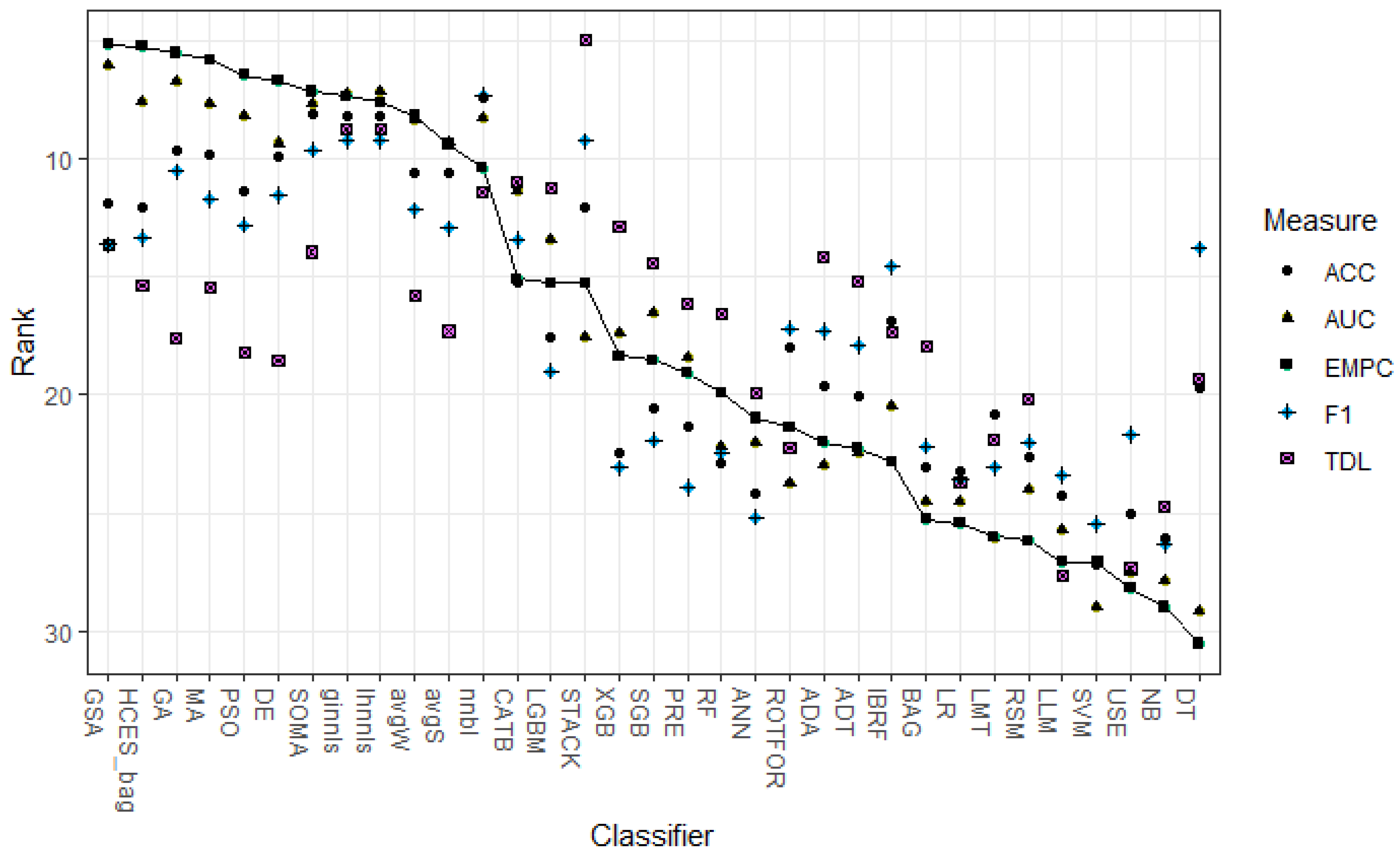
• We show that different performance measures yield different results to which classifier is most effective. For example, the statistical classifier combination methods (i.e., NNBL, LHNNLS, and GINNLS) work well for the threshold dependent metrics such as accuracy and F1 measure. These combination methods search for the coefficients that minimize the error rate, which explains their superior performance for statistical error-based metrics. For threshold independent metrics such as the AUC and EMPC, we observe that meta-heuristic search procedures (i.e., GSA, and GA) and HCES_BAG are among the top performers. These algorithms are direct optimization methods that maximize a specific metric by finding the optimal set of classifiers [94]. Hence, for threshold independent and profit/cost-based performance metrics, our results favor general purpose solvers.
• The classifiers rankings are quite robust across different sectors. A high correlation between all sectors, the telecommunications sector, and the other remaining ones is observed in terms of AUC and EMPC. For the threshold dependent metrics, the rankings vary the most between the telecommunications and other sectors. When looking at the top performing classifiers, there are variations between performance measures and sectors. Overall, the finding that statistical combination methods work best for error-based performance measures and meta-heuristics for profits still holds.
• Future studies who want to propose novel classifiers in the field of CCP should carefully benchmark their proposed method against competitive classifiers. Whereas logistic regression and random were considered the gold standard for single classifiers and homogeneous ensemble [27], our study indicates that these methods are outperformed by ANN and catboost or light GBM. Therefore, outperforming LR or RF cannot be considered as a methodological improvement. It might even be more difficult to outperform heterogeneous ensemble with GSA classifier selection, however, there is no off-the-shelf library available. Moreover, a large number of base classifiers have to be trained which can further refrain researchers from including a heterogeneous ensemble into their classifier set.
• Heterogeneous ensembles have not received much attention in CCP, and current studies mostly rely on the results of Lessmann et al. [9] and use the HCES_BAG algorithm as their default implementation. Our results, however, indicate that HCES_BAG is competitive but always outperformed by another method. Both in terms of AUC and expected profits, our results favor a heterogeneous ensemble with simulated annealing classifier selection for the local search procedures and a genetic algorithm selection for the population-based methods. For the other measures, statistical classifier selection methods such as NNBL outperform HCES_BAG. Hence, researchers that want to implement a heterogeneous ensemble method are advised to consider other methods than hill climbing. Our benchmark results can serve as a guideline for future studies.
• Our study clearly shows that putting time and effort in designing proper heterogeneous ensembles pays off: (1) adding powerful algorithms to the candidate models such as CATB and LGBM and (2) searching for the best classifier selection methods clearly increases the performance of heterogeneous ensembles.
• From a practical point of view, we show a clear trade-off between implementing simple but less accurate prediction methods (e.g., LR) or investing in advanced methods (e.g., heterogeneous ensembles) to have more accurate and profitable predictions. The results of both the statistical and Bayesian testing procedures also show that off-the-shelf methods such as CATB do not perform significantly worse than customized heterogeneous ensembles. Hence, managers should decide whether increased performance and/or profits of complex models is worth the effort.

7. Conclusions

In this research, we performed a large-scale benchmark study in customer churn prediction following other studies in related fields [9,12]. Although several studies in CCP performed a benchmark study, most of these studies introduced a novel method and compared their approach with a limited set of models specifically attuned to their situation. Moreover, single classifiers and homogenous ensembles have already been investigated thoroughly [2,6], and research regarding heterogeneous ensembles in CCP has been scarce. Because of this, the results of extant literature are often contradictory and different findings are reported across studies. [2,6].

To fill this gap in the literature, we compared 33 classifiers composed of 6 single classifiers, 14 homogeneous ensemble classifiers, and 13 heterogeneous ensemble classifiers across 11 data sets. Our findings show that the use of heterogeneous ensembles yielded better results when compared to single classifiers and homogeneous ensembles. In the majority of cases, heterogenous ensembles are ranked higher than homogenous ensembles. Moreover, this research indicates that the best heterogeneous ensemble significantly outperformed the two most popular methods in churn prediction: logistic regression and random forest. The results show that a heterogeneous ensemble optimized with generalized simulated annealing (GSA) is ranked the highest in terms of AUC and EMPC. In terms of accuracy, F1 measure and top-decile lift, a heterogeneous ensemble optimized with non-negative binomial likelihood (NNBL), and stacking are the winners. [9]

Future research could investigate several options to implement neural networks and deep learning models. This would result in an improved overview and could yield more insights. Although Gunnarsson et al. [17] showed that advanced deep learning models do not outperform XGB for credit scoring. However, other work has indicated that deep learning models can outperform random forest for customer lifetime value prediction [95]. Future studies could also deploy the classifiers on more data sets to make the results more robust. Finally, we could increase the number of base classifiers serving as candidate members for the heterogeneous ensembles [96].

References

1. Poel, D.V.D.; Larivière, B. Customer attrition analysis for financial services using proportional hazard models. Eur. J. Oper. Res. 2004, 157, 196–217. [Google Scholar] [CrossRef]
2. Verbeke, W.; Dejaeger, K.; Martens, D.; Hur, J.; Baesens, B. New insights into churn prediction in the telecommunication sector: A profit driven data mining approach. Eur. J. Oper. Res. 2012, 218, 211–229. [Google Scholar] [CrossRef]
3. Ahn, J.; Hwang, J.; Kim, D.; Choi, H.; Kang, S. A Survey on Churn Analysis in Various Business Domains. IEEE Access 2020, 8, 220816–220839. [Google Scholar] [CrossRef]
4. Ballings, M.; Poel, D.V.D. Customer event history for churn prediction: How long is long enough? Expert Syst. Appl. 2012, 39, 13517–13522. [Google Scholar] [CrossRef] [Green Version]
5. Neslin, S.A.; Gupta, S.; Kamakura, W.; Lu, J.; Mason, C.H.; Wang, C.-H.; Fong, H.-Y.; Backiel, A.; Baesens, B.; Claeskens, G.; et al. Defection Detection: Measuring and Understanding the Predictive Accuracy of Customer Churn Models. J. Mark. Res. 2006, 43, 204–211. [Google Scholar] [CrossRef] [Green Version]
6. Vafeiadis, T.; Diamantaras, K.; Sarigiannidis, G.; Chatzisavvas, K. A comparison of machine learning techniques for customer churn prediction. Simul. Model. Pract. Theory 2015, 55, 1–9. [Google Scholar] [CrossRef]
7. Coussement, K.; De Bock, K.W. Customer churn prediction in the online gambling industry: The beneficial effect of ensemble learning. J. Bus. Res. 2013, 66, 1629–1636. [Google Scholar] [CrossRef]
8. Lemmens, A.; Croux, C. Bagging and Boosting Classification Trees to Predict Churn. J. Mark. Res. 2006, 43, 276–286. [Google Scholar] [CrossRef] [Green Version]
9. Lessmann, S.; Baesens, B.; Seow, H.-V.; Thomas, L.C. Benchmarking state-of-the-art classification algorithms for credit scoring: An update of research. Eur. J. Oper. Res. 2015, 247, 124–136. [Google Scholar] [CrossRef] [Green Version]
10. Ullah, I.; Raza, B.; Malik, A.K.; Imran, M.; Islam, S.U.; Kim, S.W. A Churn Prediction Model Using Random Forest: Analysis of Machine Learning Techniques for Churn Prediction and Factor Identification in Telecom Sector. IEEE Access 2019, 7, 60134–60149. [Google Scholar] [CrossRef]
11. Wu, S.; Yau, W.-C.; Ong, T.-S.; Chong, S.-C. Integrated Churn Prediction and Customer Segmentation Framework for Telco Business. IEEE Access 2021, 9, 62118–62136. [Google Scholar] [CrossRef]
12. Baesens, B.; Van Gestel, T.; Viaene, S.; Stepanova, M.; Suykens, J.; Vanthienen, J. Benchmarking state-of-the-art classification algorithms for credit scoring. J. Oper. Res. Soc. 2003, 54, 627–635. [Google Scholar] [CrossRef]
13. de Caigny, A.; Coussement, K.; de Bock, K.W. A new hybrid classification algorithm for customer churn prediction based on logistic regression and decision trees. Eur. J. Oper. Res. 2018, 269, 760–772. [Google Scholar] [CrossRef]
14. Ke, G.; Meng, Q.; Finley, T.; Wang, T.; Chen, W.; Ma, W.; Ye, Q.; Liu, T.Y. LightGBM: A highly efficient gradient boosting decision tree. Adv. Neural Inf. Process. Syst. 2017, 30, 3147–3155. Available online: https://proceedings.neurips.cc/paper/2017/hash/6449f44a102fde848669bdd9eb6b76fa-Abstract.html (accessed on 5 August 2022).
15. Prokhorenkova, L.; Gusev, G.; Vorobev, A.; Dorogush, A.V.; Gulin, A. Catboost: Unbiased boosting with categorical features. Adv. Neural Inf. Process. Syst. 2018, 31, 6638–6648. [Google Scholar]
16. Verbraken, T.; Verbeke, W.; Baesens, B. A Novel Profit Maximizing Metric for Measuring Classification Performance of Customer Churn Prediction Models. IEEE Trans. Knowl. Data Eng. 2012, 25, 961–973. [Google Scholar] [CrossRef]
17. Gunnarsson, B.R.; Broucke, S.; Baesens, B.; Óskarsdóttir, M.; Lemahieu, W. Deep learning for credit scoring: Do or don’t? Eur. J. Oper. Res. 2021, 295, 292–305. [Google Scholar] [CrossRef]
18. Xia, Y. A Novel Reject Inference Model Using Outlier Detection and Gradient Boosting Technique in Peer-to-Peer Lending. IEEE Access 2019, 7, 92893–92907. [Google Scholar] [CrossRef]
19. Ma, X.; Sha, J.; Wang, D.; Yu, Y.; Yang, Q.; Niu, X. Study on a prediction of P2P network loan default based on the machine learning LightGBM and XGboost algorithms according to different high dimensional data cleaning. Electron. Commer. Res. Appl. 2018, 31, 24–39. [Google Scholar] [CrossRef]
20. Xia, Y.; Zhao, J.; He, L.; Li, Y.; Niu, M. A novel tree-based dynamic heterogeneous ensemble method for credit scoring. Expert Syst. Appl. 2020, 159, 113615. [Google Scholar] [CrossRef]
21. Lessmann, S.; Haupt, J.; Coussement, K.; De Bock, K.W. Targeting customers for profit: An ensemble learning framework to support marketing decision-making. Inf. Sci. 2021, 557, 286–301. [Google Scholar] [CrossRef]
22. García, S.; Fernández, A.; Luengo, J.; Herrera, F. Advanced nonparametric tests for multiple comparisons in the design of experiments in computational intelligence and data mining: Experimental analysis of power. Inf. Sci. (N. Y.) 2010, 180, 2044–2064. [Google Scholar] [CrossRef]
23. Benavoli, A.; Corani, G.; Demšar, J.; Zaffalon, M. Time for a Change: A Tutorial for Comparing Multiple Classifiers through Bayesian Analysis. J. Mach. Learn. Res. 2017, 136–181. [Google Scholar]
24. Woźniak, M.; Graña, M.; Corchado, E. A survey of multiple classifier systems as hybrid systems. Inf. Fusion 2014, 16, 3–17. [Google Scholar] [CrossRef] [Green Version]
25. Dietterich, T.G. Ensemble Methods in Machine Learning. In Multiple Classifier Systems: First International Workshop, MCS 2000 Proceedings 1, Cagliari, Italy, 21–23 June 2000; Lecture Notes in Computer Science (Including Subseries Lecture Notes in Artificial Intelligence and Lecture Notes in Bioinformatics), 1857 LNCS; Springer: Berlin/Heidelberg, Germany, 2000; pp. 1–15. [Google Scholar]
26. Nascimento, D.S.; Coelho, A.L.; Canuto, A.M. Integrating complementary techniques for promoting diversity in classifier ensembles: A systematic study. Neurocomputing 2014, 138, 347–357. [Google Scholar] [CrossRef]
27. Coussement, K.; Lessmann, S.; Verstraeten, G. A comparative analysis of data preparation algorithms for customer churn prediction: A case study in the telecommunication industry. Decis. Support Syst. 2017, 95, 27–36. [Google Scholar] [CrossRef]
28. Mirkovic, M.; Lolic, T.; Stefanovic, D.; Anderla, A.; Gracanin, D. Customer Churn Prediction in B2B Non-Contractual Business Settings Using Invoice Data. Appl. Sci. 2022, 12, 5001. [Google Scholar] [CrossRef]
29. Burez, J.; Poel, D.V.D. CRM at a pay-TV company: Using analytical models to reduce customer attrition by targeted marketing for subscription services. Expert Syst. Appl. 2007, 32, 277–288. [Google Scholar] [CrossRef] [Green Version]
30. Hung, S.-Y.; Yen, D.C.; Wang, H.-Y. Applying data mining to telecom churn management. Expert Syst. Appl. 2006, 31, 515–524. [Google Scholar] [CrossRef] [Green Version]
31. Moeyersoms, J.; Martens, D. Including high-cardinality attributes in predictive models: A case study in churn prediction in the energy sector. Decis. Support Syst. 2015, 72, 72–81. [Google Scholar] [CrossRef]
32. Tsai, C.-F.; Lu, Y.-H. Customer churn prediction by hybrid neural networks. Expert Syst. Appl. 2009, 36, 12547–12553. [Google Scholar] [CrossRef]
33. Baumann, A.; Lessmann, S.; Coussement, K.; De Bock, K.W.; Bock, D. Maximize What Matters: Predicting Customer Churn with Decision-Centric Ensemble Selection; Association for Information Systems AIS Electronic Library (AISeL): Münster, Germany, 2015; pp. 1–15. [Google Scholar]
34. Bogaert, M.; Ballings, M.; Poel, D.V.D. Evaluating the importance of different communication types in romantic tie prediction on social media. Ann. Oper. Res. 2016, 263, 501–527. [Google Scholar] [CrossRef]
35. Óskarsdóttir, M.; Bravo, C.; Verbeke, W.; Sarraute, C.; Baesens, B.; Vanthienen, J. Social network analytics for churn prediction in telco: Model building, evaluation and network architecture. Expert Syst. Appl. 2017, 85, 204–220. [Google Scholar] [CrossRef] [Green Version]
36. Demšar, J. Statistical Comparisons of Classifiers over Multiple Data Sets. J. Mach. Learn. Res. 2006, 7, 1–30. [Google Scholar]
37. Xia, Y.; Liu, C.; Da, B.; Xie, F. A novel heterogeneous ensemble credit scoring model based on bstacking approach. Expert Syst. Appl. 2018, 93, 182–199. [Google Scholar] [CrossRef]
38. de Bock, K.W.; de Caigny, A. Spline-rule ensemble classifiers with structured sparsity regularization for interpretable customer churn modeling. Decis. Support Syst. 2021, 150, 113523. [Google Scholar] [CrossRef]
39. Buckinx, W.; Poel, D.V.D. Customer base analysis: Partial defection of behaviourally loyal clients in a non-contractual FMCG retail setting. Eur. J. Oper. Res. 2005, 164, 252–268. [Google Scholar] [CrossRef]
40. Coussement, K.; Poel, D.V.D. Churn prediction in subscription services: An application of support vector machines while comparing two parameter-selection techniques. Expert Syst. Appl. 2008, 34, 313–327. [Google Scholar] [CrossRef]
41. Burez, J.; Van den Poel, D. Handling class imbalance in customer churn prediction. Expert Syst. Appl. 2009, 36, 4626–4636. [Google Scholar] [CrossRef] [Green Version]
42. Xie, Y.; Li, X.; Ngai, E.; Ying, W. Customer churn prediction using improved balanced random forests. Expert Syst. Appl. 2009, 36, 5445–5449. [Google Scholar] [CrossRef]
43. De Bock, K.W.; Poel, D.V.D. An empirical evaluation of rotation-based ensemble classifiers for customer churn prediction. Expert Syst. Appl. 2011, 38, 12293–12301. [Google Scholar] [CrossRef]
44. De Bock, K.W.; Poel, D.V.D. Reconciling performance and interpretability in customer churn prediction using ensemble learning based on generalized additive models. Expert Syst. Appl. 2012, 39, 6816–6826. [Google Scholar] [CrossRef]
45. Kim, N.; Jung, K.-H.; Kim, Y.S.; Lee, J. Uniformly subsampled ensemble (USE) for churn management: Theory and implementation. Expert Syst. Appl. 2012, 39, 11839–11845. [Google Scholar] [CrossRef]
46. Idris, A.; Rizwan, M.; Khan, A. Churn prediction in telecom using Random Forest and PSO based data balancing in combination with various feature selection strategies. Comput. Electr. Eng. 2012, 38, 1808–1819. [Google Scholar] [CrossRef]
47. Idris, A.; Khan, A. Churn Prediction System for Telecom using Filter–Wrapper and Ensemble Classification. Comput. J. 2016, 60, 410–430. [Google Scholar] [CrossRef]
48. Zhu, B.; Broucke, S.; Baesens, B.; Maldonado, S. Improving Resampling-based Ensemble in Churn Prediction. In Proceedings of the Machine Learning Research, PMLR, London, UK, 11 October 2017; Volume 74, pp. 79–91. Available online: http://proceedings.mlr.press/v74/zhu17a.html (accessed on 9 August 2021).
49. Zhu, B.; Baesens, B.; vanden Broucke, S.K. An empirical comparison of techniques for the class imbalance problem in churn prediction. Inf. Sci. 2017, 408, 84–99. [Google Scholar] [CrossRef] [Green Version]
50. Zhu, B.; Baesens, B.; Backiel, A.; Broucke, S.K.L.M.V. Benchmarking sampling techniques for imbalance learning in churn prediction. J. Oper. Res. Soc. 2018, 69, 49–65. [Google Scholar] [CrossRef] [Green Version]
51. Jain, H.; Khunteta, A.; Srivastava, S. Churn Prediction in Telecommunication using Logistic Regression and Logit Boost. Procedia Comput. Sci. 2020, 167, 101–112. [Google Scholar] [CrossRef]
52. Bhujbal, N.S.; Bavdane, G.P. Leveraging the efficiency of Ensembles for Customer Retention. In Proceedings of the 5th International Conference on I-SMAC (IoT in Social, Mobile, Analytics and Cloud), I-SMAC 2021, Palladam, India, 11–13 November 2021; pp. 1675–1679. [Google Scholar]
53. Chowdhury, A.; Kaisar, S.; Rashid, M.; Shafin, S.S.; Kamruzzaman, J. Churn Prediction in Telecom Industry using Machine Learning Ensembles with Class Balancing. In Proceedings of the 2021 IEEE Asia-Pacific Conference on Computer Science and Data Engineering (CSDE), Brisbane, Australia, 8–10 December 2021; pp. 1–6. [Google Scholar] [CrossRef]
54. Deng, Y.; Li, D.; Yang, L.; Tang, J.; Zhao, J. Analysis and prediction of bank user churn based on ensemble learning algorithm. In Proceedings of the 2021 IEEE International Conference on Power Electronics, Computer Applications (ICPECA), Shenyang, China, 22–24 January 2021. [Google Scholar] [CrossRef]
55. Janssens, B.; Bogaert, M.; Bagué, A.; van den Poel, D. B2Boost: Instance-dependent profit-driven modelling of B2B churn. Ann. Oper. Res. 2022, 1–27. [Google Scholar] [CrossRef]
56. Karuppaiah, K.S.; Palanisamy, N.G. WITHDRAWN: Heterogeneous ensemble stacking with minority upliftment (HESMU) for churn prediction on imbalanced telecom data. Mater. Today Proc. 2021. [Google Scholar] [CrossRef]
57. Kiguchi, M.; Saeed, W.; Medi, I. Churn prediction in digital game-based learning using data mining techniques: Logistic regression, decision tree, and random forest. Appl. Soft. Comput. 2022, 118, 108491. [Google Scholar] [CrossRef]
58. Sagala, N.T.M.; Permai, S.D. Enhanced Churn Prediction Model with Boosted Trees Algorithms in The Banking Sector. In Proceedings of the 2021 International Conference on Data Science and Its Applications (ICoDSA), Bandung, Indonesia, 6–7 October 2021; pp. 240–245. [Google Scholar] [CrossRef]
59. Vo, N.N.; Liu, S.; Li, X.; Xu, G. Leveraging unstructured call log data for customer churn prediction. Knowl.-Based Syst. 2021, 212, 106586. [Google Scholar] [CrossRef]
60. Gattermann-Itschert, T.; Thonemann, U.W. How training on multiple time slices improves performance in churn prediction. Eur. J. Oper. Res. 2021, 295, 664–674. [Google Scholar] [CrossRef]
61. Corani, G.; Benavoli, A. A Bayesian approach for comparing cross-validated algorithms on multiple data sets. Mach. Learn. 2015, 100, 285–304. [Google Scholar] [CrossRef] [Green Version]
62. Van Belle, R.; Baesens, B.; De Weerdt, J. CATCHM: A novel network-based credit card fraud detection method using node representation learning. Decis. Support Syst. 2022, 164, 113866. [Google Scholar] [CrossRef]
63. Breiman, L. Bagging predictors. Mach. Learn. 1996, 24, 123–140. [Google Scholar] [CrossRef] [Green Version]
64. Nie, G.; Rowe, W.; Zhang, L.; Tian, Y.; Shi, Y. Credit card churn forecasting by logistic regression and decision tree. Expert Syst. Appl. 2011, 38, 15273–15285. [Google Scholar] [CrossRef]
65. Ballings, M.; Poel, D.V.D. Kernel Factory: An ensemble of kernel machines. Expert Syst. Appl. 2013, 40, 2904–2913. [Google Scholar] [CrossRef]
66. Porwik, P.; Doroz, R.; Wrobel, K. An ensemble learning approach to lip-based biometric verification, with a dynamic selection of classifiers. Expert Syst. Appl. 2019, 115, 673–683. [Google Scholar] [CrossRef]
67. Bryll, R.; Gutierrez-Osuna, R.; Quek, F. Attribute bagging: Improving accuracy of classifier ensembles by using random feature subsets. Pattern Recognit. 2003, 36, 1291–1302. [Google Scholar] [CrossRef]
68. Breiman, L. Random forests. Mach. Learn. 2001, 45, 5–32. [Google Scholar] [CrossRef] [Green Version]
69. Bogaert, M.; Ballings, M.; Poel, D.V.D.; Oztekin, A. Box office sales and social media: A cross-platform comparison of predictive ability and mechanisms. Decis. Support Syst. 2021, 147, 113517. [Google Scholar] [CrossRef]
70. Friedman, J.H. Stochastic gradient boosting. Comput. Stat. Data Anal. 2002, 38, 367–378. [Google Scholar] [CrossRef]
71. Ballings, M.; Poel, D.V.D. CRM in social media: Predicting increases in Facebook usage frequency. Eur. J. Oper. Res. 2015, 244, 248–260. [Google Scholar] [CrossRef]
72. Chen, T.; Guestrin, C. XGBoost: A scalable tree boosting system. In Proceedings of the ACM SIGKDD International Conference on Knowledge Discovery and Data Mining, San Francisco, CA, USA, 13–17 August 2016; pp. 785–794. [Google Scholar]
73. Landwehr, N.; Hall, M.; Frank, E. Logistic Model Trees. Mach. Learn. 2005, 59, 161–205. [Google Scholar] [CrossRef] [Green Version]
74. Fokkema, M. Fitting Prediction Rule Ensembles with R Package pre. J. Stat. Softw. 2020, 92, 1–30. [Google Scholar] [CrossRef] [Green Version]
75. Freund, Y.; Mason, L. The alternating decision tree learning algorithm. In ICML; Morgan Kaufmann Publishers Inc.: San Francisco, CA, USA, 1999; Volume 99, pp. 124–133. [Google Scholar]
76. Wang, R.; Na Cheng, M.; Loh, Y.M.; Wang, C.; Cheung, C.F. Ensemble learning with a genetic algorithm for surface roughness prediction in multi-jet polishing. Expert Syst. Appl. 2022, 207, 118024. [Google Scholar] [CrossRef]
77. Rahman, A.; Verma, B. Ensemble classifier generation using non-uniform layered clustering and Genetic Algorithm. Knowl.-Based Syst. 2013, 43, 30–42. [Google Scholar] [CrossRef]
78. Ballings, M.; Poel, D.V.D.; Bogaert, M. Social media optimization: Identifying an optimal strategy for increasing network size on Facebook. Omega 2016, 59, 15–25. [Google Scholar] [CrossRef]
79. Zhou, Z.-H.; Wu, J.; Tang, W. Ensembling neural networks: Many could be better than all. Artif. Intell. 2002, 137, 239–263. [Google Scholar] [CrossRef] [Green Version]
80. Xue, B.; Zhang, M.; Browne, W.N. Particle swarm optimisation for feature selection in classification: Novel initialisation and updating mechanisms. Appl. Soft Comput. 2014, 18, 261–276. [Google Scholar] [CrossRef]
81. Zainudin, M.; Sulaiman, M.; Mustapha, N.; Perumal, T.; Nazri, A.; Mohamed, R.; Manaf, S. Feature Selection Optimization using Hybrid Relief-f with Self-adaptive Differential Evolution. Int. J. Intell. Eng. Syst. 2017, 10, 21–29. [Google Scholar] [CrossRef]
82. Meiri, R.; Zahavi, J. Using simulated annealing to optimize the feature selection problem in marketing applications. Eur. J. Oper. Res. 2006, 171, 842–858. [Google Scholar] [CrossRef]
83. Molina, D.; Lozano, M.; García-Martínez, C.; Herrera, F. Memetic Algorithms for Continuous Optimisation Based on Local Search Chains. Evol. Comput. 2010, 18, 27–63. [Google Scholar] [CrossRef] [PubMed]
84. Ballings, M. Advances and Applications in Ensemble Learning; Ghent University, Faculty of Economics and Business Administration: Ghent, Belgium, 2014. [Google Scholar]
85. Coussement, K.; Buckinx, W. A probability-mapping algorithm for calibrating the posterior probabilities: A direct marketing application. Eur. J. Oper. Res. 2011, 214, 732–738. [Google Scholar] [CrossRef]
86. Cheng, N.; Wang, H.; Tang, X.; Zhang, T.; Gui, J.; Zheng, C.-H.; Xia, J. An Ensemble Framework for Improving the Prediction of Deleterious Synonymous Mutation. IEEE Trans. Circuits Syst. Video Technol. 2021, 32, 2603–2611. [Google Scholar] [CrossRef]
87. De, S.; Prabu, P. A Sampling-Based Stack Framework for Imbalanced Learning in Churn Prediction. IEEE Access 2022, 10, 68017–68028. [Google Scholar] [CrossRef]
88. Bin, Y.; Zhang, W.; Tang, W.; Dai, R.; Li, M.; Zhu, Q.; Xia, J. Prediction of Neuropeptides from Sequence Information Using Ensemble Classifier and Hybrid Features. J. Proteome Res. 2020, 19, 3732–3740. [Google Scholar] [CrossRef]
89. Amin, A.; Al-Obeidat, F.; Shah, B.; Adnan, A.; Loo, J.; Anwar, S. Customer churn prediction in telecommunication industry using data certainty. J. Bus. Res. 2019, 94, 290–301. [Google Scholar] [CrossRef]
90. Ahmed, M.; Siddiqi, I.; Afzal, H.; Khan, B. MCS: Multiple classifier system to predict the churners in the telecom industry. In Proceedings of the 2017 Intelligent Systems Conference (IntelliSys), London, UK, 7–8 September 2017; pp. 678–683. [Google Scholar] [CrossRef]
91. Bogaert, M.; Lootens, J.; Poel, D.V.D.; Ballings, M. Evaluating multi-label classifiers and recommender systems in the financial service sector. Eur. J. Oper. Res. 2019, 279, 620–634. [Google Scholar] [CrossRef]
92. Schetgen, L.; Bogaert, M.; Poel, D.V.D. Predicting donation behavior: Acquisition modeling in the nonprofit sector using Facebook data. Decis. Support Syst. 2021, 141, 113446. [Google Scholar] [CrossRef]
93. Carrasco, J.; García, S.; del Mar Rueda, M.; Herrera, F. rNPBST: An R Package Covering Non-parametric and Bayesian Statistical Tests. In Hybrid Artificial Intelligent Systems: 12th International Conference, HAIS 2017 Proceedings 12, La Rioja, Spain, 21–23 June 2017; Lecture Notes in Computer Science (including subseries Lecture Notes in Artificial Intelligence and Lecture Notes in Bioinformatics), 10334 LNCS; Springer International Publishing: Berlin/Heidelberg, Germany, 2017; pp. 281–292. [Google Scholar]
94. De Bock, K.W.; Coussement, K.; Lessmann, S. Cost-sensitive business failure prediction when misclassification costs are uncertain: A heterogeneous ensemble selection approach. Eur. J. Oper. Res. 2020, 285, 612–630. [Google Scholar] [CrossRef]
95. Benk, G.Y.; Badur, B.; Mardikyan, S. A New 360° Framework to Predict Customer Lifetime Value for Multi-Category E-Commerce Companies Using a Multi-Output Deep Neural Network and Explainable Artificial Intelligence. Information 2022, 13, 373. [Google Scholar] [CrossRef]
96. Abellán, J.; Castellano, J.G. A comparative study on base classifiers in ensemble methods for credit scoring. Expert Syst. Appl. 2017, 73, 1–10. [Google Scholar] [CrossRef]
Figure 1. Graphical depiction of the main principles of our proposed heterogeneous ensemble framework.
Mathematics 11 01137 g001
Figure 2. The average rank across 11 data sets for each classifier for each performance measure.
Mathematics 11 01137 g002
Figure 3. Posterior distribution with ROPE of the Bayesian analysis of LR and LHNLS.
Mathematics 11 01137 g003