Article

A New Dual Normalization for Enhancing the Bitcoin Pricing Capability of an Optimized Low Complexity Neural Net with TOPSIS Evaluation

Department of Computer Science and Engineering, Siksha ‘O’ Anusandhan (Deemed to be) University, Bhubaneswar 751030, Odisha, India
*
Author to whom correspondence should be addressed.
Mathematics 2023, 11(5), 1134; https://doi.org/10.3390/math11051134
Submission received: 31 December 2022 / Revised: 8 February 2023 / Accepted: 21 February 2023 / Published: 24 February 2023

Abstract

:
Bitcoin, the largest cryptocurrency, is extremely volatile and hence needs a better model for its pricing. In the literature, many researchers have studied the effect of data normalization on regression analysis for stock price prediction. How has data normalization affected Bitcoin price prediction? To answer this question, this study analyzed the prediction accuracy of a Legendre polynomial-based neural network optimized by the mutated climb monkey algorithm using nine existing data normalization techniques. A new dual normalization technique was proposed to improve the efficiency of this model. The 10 normalization techniques were evaluated using 15 error metrics using a multi-criteria decision-making (MCDM) approach called technique for order performance by similarity to ideal solution (TOPSIS). The effect of the top three normalization techniques along with the min–max normalization was further studied for Chebyshev, Laguerre, and trigonometric polynomial-based neural networks in three different datasets. The prediction accuracy of the 16 models (each of the four polynomial-based neural networks with four different normalization techniques) was calculated using 15 error metrics. A 16 × 15 TOPSIS analysis was conducted to rank the models. The convergence plot and the ranking of the models indicated that data normalization plays a significant role in the prediction capability of a Bitcoin price predictor. This paper can significantly contribute to the research with a new normalization technique for utilization in varied fields of research. It can also contribute to international finance as a decision-making tool for different investors as well as stakeholders for Bitcoin pricing.

1. Introduction

Digitization of the global economy is steadily progressing into a new future. We are shifting from traditional ways of transacting and investing to digitized ones. This signifies the importance of digital currency in the current economic scenario. Nowadays, every business wants a more digitized form of implementation using digital technology in some forms. To enhance their efficiency, many business enterprises are using digital information systems and software such as Systems Applications and Products (SAP) [1]. To explore the benefits of digital currency, a review of centralization in a decentralized ledger is extensively presented [2]. Such currency can be assumed to be goods as well as money at a time and is known as cryptocurrency [3].
However, the growth of the Bitcoin market is heavily affected by its volatility. It is eight times more volatile than the stock market. Many investors and stakeholders are still very skeptical about the acceptance of Bitcoin as a reliable asset. A better model for predicting Bitcoin price can be a great help in the expansion of the crypto market. Many researchers have used various artificial neural networks (ANNs)-based models for Bitcoin prediction. A few machine learning and deep learning methods have been used to predict the Bitcoin prices as well as other cryptocurrencies [4,5,6]. We proposed a low complexity polynomial-based neural network optimized by a new mutated climb monkey algorithm for an efficient prediction of daily Bitcoin closing price [7]. Baser and Sadorsky [8] studied the effect of technical indicators, macroeconomic variables and multi-step forecast horizon (from 1 day to 20 days) on Bitcoin price direction prediction using random forests. Erfanian et al. [9] analyzed and compared the forecasting efficiency of machine learning algorithms with statistical analysis by using technical indicators, microeconomic variables, and macroeconomic variables for short-term and long-term Bitcoin price prediction. Rathore et al. [10] demonstrated the qualitative prediction of Bitcoin price by using seasonal inputs for training.
Although many recent studies have addressed the volatility of Bitcoin price by using different input variables, machine learning, and deep learning algorithms, there is very little literature available that predicts the Bitcoin price by analyzing the data preprocessing techniques.
Data preprocessing is a process of cleaning, reducing, extracting, scaling, and handling missing values in a raw dataset. Many researchers have used feature extraction methods to improve the prediction accuracy of Bitcoin [11,12]. Rajabi et al. [13] proposed the use of deep learning in selecting an optimal window size for prediction and then using the optimal size for actual Bitcoin price forecasting.
Data normalization is a vital preprocessing step for the majority of classification and regression problems. This method utilizes various ways to map the highly volatile data to a limited range to improve the prediction capability of various models. In the literature, Shanker et al. [14] studied the data standardization on the training of a neural network and concluded that with the increase in network size, the self-scalability of the network increases, and hence, there is no effect of scalability on network performance.
In contrast, many researchers have demonstrated the significant role played by various data-scaling methods in classification problems [15,16]. It has been observed that the data normalization type may be used to improve classification accuracy. Some researchers have studied the impact of various normalization techniques on stock price prediction and had suggested that the data normalization type plays a very significant role in prediction and so it should be appropriately selected [17,18].
However, the effect of data normalization on Bitcoin pricing is yet to be analyzed. As the Bitcoin price is highly volatile, to obtain an efficient model for prediction, the normalization of the Bitcoin dataset needs to be explored. The main goal of this investigation is to analyze the influence of data normalization techniques on the prediction capability of a Bitcoin price predictor. Namely, this study investigated the effect of nine different data normalization techniques on the Legendre-based neural network model for daily Bitcoin price prediction.
The novelty of this approach is that it proposes a new dual normalization technique for efficient Bitcoin price prediction. Hybrid normalizations have been extensively used in the medical domain, but in cryptocurrency prediction, researchers have mostly used min–max normalization or z-score normalization. This is the first paper to suggest the analysis of 10 normalization methods using 15 performance metrics for efficient Bitcoin price prediction.
The main contributions of this paper are enlisted as follows:
  • Nine data normalization types were used to process three different datasets.
  • Each normalized dataset was used as input for the Legendre-based polynomial neural network model trained by the mutated climb monkey algorithm (LMCMA) to predict the closing Bitcoin price.
  • A new dual normalization technique was proposed for an improved prediction.
  • The proposed normalization technique was tested in three different functional link neural networks, an econometric model and a Support Vector Regression model
  • A TOPSIS-based approach was applied for ranking the normalization type using 15 performance criteria.
  • The LMCMA model with the proposed dual normalization was also tested for predicting daily Bitcoin log returns for the three datasets under study.
This empirical research analyzed the following research hypotheses:
Hypothesis 1. 
There is a significant relationship between data normalization and prediction accuracy of Bitcoin Price Predictor models.
Hypothesis 2. 
A dual normalization improves the prediction capability of Bitcoin price predictor models.
The research methodology is varied in that the Bitcoin predictor models in this study were evaluated using a TOPSIS-based ranking. In addition, the models used datasets scaled using a new normalization technique.
The importance of this research lies in the need for a highly efficient predictor for Bitcoin prices to handle the high volatility feature of Bitcoin prices. The research proposes a dual normalization that significantly improves the accuracy of prediction of Bitcoin closing price as well as daily log returns. The use of the new normalization technique indicated a root mean square error gain of 81.37%, 98.13%, and 98.73% over min–max normalization in the Bitfinex, Binance, and Coinbase Pro datasets, respectively.
Section 2 gives a review of the literature on Bitcoin pricing and normalization techniques used in this paper. Section 3 introduces the basic model used in this study. Section 4 explains the workflow of this study along with explanations of related techniques. It then introduces the proposed normalization and the experimental setup. Section 5 presents the experimental results followed by a thorough discussion in Section 6. The last section concludes this study and suggests various open research issues for future work.

2. Literature Review

Bitcoin is highly volatile and dynamic in nature. Many forecasting models have been presented using machine learning for Bitcoin price prediction. The volatility has been proved by a study of a Support Vector Machine (SVM)-based predictor [19]. Aggarwal et al. [20] demonstrated Bitcoin pricing using an SVM and ensemble approach. Many researchers have used LSTM and Bayesian networks for Bitcoin prediction [6,9]. Deep learning has also been used to predict Bitcoin prices efficiently by using autoencoders and LSTM [5,21]. Rathore et al. [10] have presented a more real-world model by using a FbProphet model for better prediction in comparison to LSTM.
Recently, we proposed a functional artificial link neural network (FLANN) based on Chebyshev and Legendre polynomial functions as a simple yet efficient model for Bitcoin pricing [7]. An optimal FLANN has been proposed to predict Bitcoin price movement by using a genetic algorithm-based optimization of the network [6].
Nayak et al. [22] presented the hybridization of high-order neural network (HONN) models with the evolutionary algorithms for efficient stock price prediction. They have explained the reliable and simple architecture of various HONNs such as pi-sigma neural network (PSNN), sigma-pi neural network (SPNN), and FLANNs based on Chebyshev, Laguerre, and Legendre polynomials. Ye et al. [23] presented a stable and more accurate wind power forecasting using a Laguerre polynomials-based neural network. Many other researchers have utilized the flat architecture, fast learning capabilities, and reliable features of FLANN models for stock price, gold price, and mutual fund net asset value prediction [24,25,26,27,28,29]. This motivated us to use the LMCMA model for Bitcoin prediction in this study [7].
In the literature, many researchers have studied the effect of data normalization on various classifications, regression, and decision-making models. Jain et al. [30] explored min–max and z-score normalization with 12 data complexity measures in 14 classification models to find the best normalization selected dynamically. They used Friedman’s test for evaluation [31]. Alshdaifat et al. [32] analyzed three normalization methods with three missing value handling methods on nine different ANN and SVM models for 18 benchmark datasets. They concluded that the z-score performed the best and decimal scaling was the worst normalization under study. The evaluation was based on Friedman’s test and Nemenyi’s posthoc test [33]. Singh and Singh [16] investigated 14 normalization methods to study their effect on classification accuracy by integrating normalization with weighted features. In [34], they proposed a feature-wise normalization technique. They explained that entire data normalization can be replaced with feature-wise normalization for efficient training.
Sola and Sevilla [35] studied the impact of data normalization on two neural networks trained by using backpropagation in nuclear power plant applications and concluded that normalization reduces errors and error computation time as well as enhances the network performance. The effect of normalization has been studied for many other applications such as linear ordering and 2Dcoordinate transformation [36,37].
The selection of normalization also plays a vital role in enhancing the performance of multi-criteria decision-making models (MCDM) [38,39,40]. The ranking process of MCDM models is also enhanced by selecting the appropriate normalization technique [41,42].
Very few hybrid normalization techniques have been proposed by combining different available normalization methods [41,43]. Recently, Izonin et al. [44] proposed two-step normalization by combining max-abs scaler and vector scaler, which improved the classification accuracy for medical applications. This motivated us to study the effect of normalization on Bitcoin pricing and propose a new dual normalization technique for enhanced prediction capability.
In the literature, econometric models have been extensively used in the finance domain. Batrancea [45] demonstrated the effectiveness of two econometric models in predicting the influence of many economic indicators on liquidity and solvency ratios in the healthcare industries. In [46], the influence of the financial statement of a bank on its assets, liabilities, and performance is analyzed using an econometric model. For Bitcoin price prediction, many studies have been used to study the impact of technical indicators and macroeconomic indicators. In [9], the effect of technical, macroeconomic, microstructure, and blockchain indicators on Bitcoin pricing has been analyzed using SVR (Support Vector Regression), MLP, OLS and an ensemble model. The SVR model was efficient in comparison to other models.
In light of the above review, it can be stated that this research will be very useful in the designing of new models by researchers for efficient prediction using the proposed dual normalization. In addition, it can help investors make decisions on Bitcoin investment with a more accurate prediction of future prices.

3. Materials and Methods

In [7], we proposed the use of a new mutated climb monkey algorithm-based Legendre neural network (LMCMA) model for efficient Bitcoin pricing. This model uses the benefits of a FLANN with efficient training capability of the MCMA algorithm. The basic architecture of the LMCMA model is shown in Figure 1.
The LMCMA model contains an input expansion block (IEB) which expands each input x to expanded polynomials Li(x) where i = 1, 2, … r, for expansion order r. This model utilizes polynomial expansion of order 2. As shown in Figure 1, the inputs x1 and x2 are expanded into L1(x1), L2(x1) and L1(x2), L2(x2), respectively, for r = 2. A random weight matrix is applied to the expanded inputs. The weighted sum of the expanded input is passed to the tanh activation function. It derives the predicted output, which is then subtracted from the actual output to generate an error. This error is used by the MCMA algorithm for weight updates.
In this model, the expanded Legendre polynomials are generated by using the recursive formula given in Equation (1):
L i + 1 ( x ) = 1 i + 1 × [ ( 2 i + 1 ) × x × L i ( x ) i × L i 1 ( x ) ]
where x is the input data and Li represents the ith Legendre polynomial for i = 0, 1, 2, … and L0(x) = 1 and L1(x) = x.
After training the model, the optimized weight giving minimum root mean square error (RMSE) is frozen for testing the network for the test dataset.
The MCMA algorithm used in this model uses a mutated climb operation in the original monkey algorithm. This reduces the time spent on the climb operation and also gives optimal weights for prediction [7].

4. Proposed Work

This section describes the steps involved in this study. It then provides a dataset analysis of the used datasets. The succeeding subsection describes the normalization types used in this study and their analysis. It is followed by the new proposed normalization and the performance evaluation methods involved in this study.

4.1. Procedural Analysis

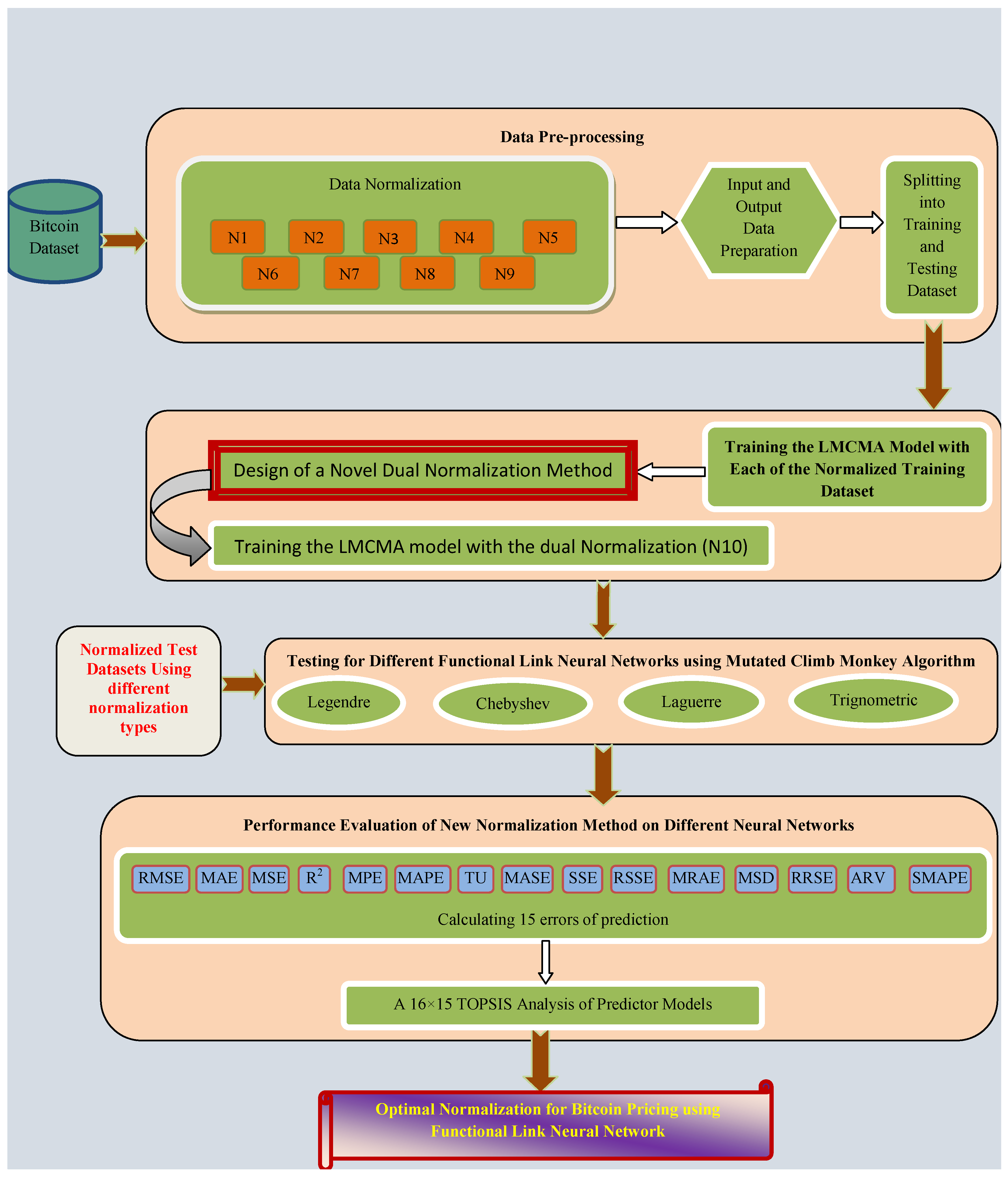
This study analyzes the normalization types for the prediction of Bitcoin prices and then proposes a new normalization type. The steps involved in this study are presented in Figure 2.
The proposed study starts with normalizing the datasets using nine normalization methods. The normalized dataset is then divided into input and output data using the sliding window technique. The data are then divided into training and testing datasets.
The LMCMA model is then trained using each of the normalized training datasets. The minimum RMSE for each normalized training dataset is calculated, and the best two normalization types are used to design a dual normalization technique. The LMCMA model is then trained on the new normalized dataset. All 10 normalization techniques are applied on testing datasets and then evaluated based on 15 different error metrics. The top-ranked normalization along with the min–max normalization technique, which was originally proposed in the LMCMA model [7], is then tested with three other FLANNs.
The recursive Chebyshev polynomials are generated using Equation (2):
C i + 1 ( x ) = 2 × x × C i ( x ) C i 1 ( x )
where x is the input data and Ci represents the ith Chebyshev polynomial for i = 0, 1, 2, … and C0(x) = 1 and C1(x) = x.
The recursive Laguerre polynomials are generated using Equation (3):
La i + 1 ( x ) = 1 i + 1 × [ ( 2 i + 1 ) × La i ( x ) i × La i 1 ( x ) ]
where x is the input data and Lai represents the ith Laguerre polynomial for i = 0, 1, 2, … and La0(x) = 1 and La1(x) = 1 − x.
The trigonometric functions used for input expansion are described in Equation (4):
T1(x) = x, T2(x) = sine(x), T3(x) = cosine(x), T4(x) = sine(πx), T5(x) = cosine(πx)
After testing the four networks with min–max normalization, the proposed dual normalization, and the top two ranked normalization ranked in the training of the LMCMA model were evaluated using 15 error measures. A 16 × 15 TOPSIS analysis was conducted to select the best normalization technique in a FLANN model.

4.2. Dataset Analysis

For the simulation of this study, historical daily closing Bitcoin prices in US dollars (USD) were collected from http://www.investing.com/crypto/bitcoin/historical-data (accessed on 15 November 2022) for three different crypto-markets. They are Bitfinex, Binance and, Coinbase Pro datasets. The most recent data were collected for this study within the time range of 15 November 2018 to 15 November 2022. The datasets cover prices from pre-COVID to post-COVID durations and hence map the high volatility. The dataset descriptions are shown in Table 1.
The datasets were analyzed statistically to obtain an insight into the data represented in each of the datasets. The statistical analysis of the three datasets is presented in Table 2.

4.3. Normalization Methods

Data normalization is a vital process in any regression analysis. It transforms data into a fixed interval to decrease the training time and errors. This study analyzes the impact of nine data normalization techniques in the LMCMA model for the prediction of Bitcoin closing prices.

4.3.1. Min–Max Normalization

Most of the regression analysis uses the min–max normalization technique. It is a process of converting data by using the minimum and maximum values in a dataset [7,47]. The normalized data are calculated by using Equation (5):
x = x min max min
where x is the original data, x′ is the normalized data, and min and max represent the minimum and maximum values in the dataset, respectively.

4.3.2. Decimal Scaling

In decimal scaling normalization, each data is normalized using a maximum value of a dataset and the radix of the dataset used [32,48]. The normalized data are calculated by using Equation (6):
x = x 10 d
where x is the original data, x′ is the normalized data and d is the number of digits present in the maximum value of the dataset.

4.3.3. Vector Normalization

Vector normalization is a sum-based normalization. Here, the data are transformed by using the absolute sum of the squares of each data [44,49]. The normalized data are calculated by using Equation (7):
x = x 1 n | X | 2
where x is the original data, x′ is the normalized data and n is the total number of data in dataset X.

4.3.4. Maximum Linear Normalization

The maximum linear normalization is also known as MaxAbs Scaler. It uses absolute values for mapping [44,50]. This normalization is based on the maximum value in the dataset. The normalized data are calculated by using Equation (8).
x = x max ( | X | )
where x is the original data, x′ is the normalized data and max(X) is a function to find themaximum value in dataset X.

4.3.5. Juttler–Korth Normalization

In this normalization, the data are normalized using the maximum value in the dataset. It also uses the absolute values of the data for normalization [49,51]. The normalized data are calculated by using Equation (9):
x = 1 | max ( | X | ) x max ( X ) |
where x is the original data, x′ is the normalized data and max(X) is a function to find the maximum value in dataset X.

4.3.6. Peldschus Normalization

This is a square-based normalization technique that also uses the maximum value in a dataset for scaling [49,51]. The normalized data are calculated by using Equation (10):
x = ( x max ( X ) ) 2
where x is the original data, x′ is the normalized data and max(X) is a function to find the maximum value in dataset X.

4.3.7. Tanh Estimator

A tanh estimator is an efficient normalization technique based on the mean and standard deviation of the dataset [52]. This normalization has been used in many stock price predictions. The normalized data are calculated by using Equation (11):
x = 0.5 × [ tanh [ 0.01 × ( x μ ) σ + 1 ] ]
where x is the original data, x′ is the normalized data, and μ and σ are the mean and standard deviation of dataset X, respectively.

4.3.8. Logistic Sigmoidal Normalization

This normalization is based on the mean and standard deviation of the dataset. It uses a sigmoidal-based approach for normalization [53]. The normalized data are calculated by using Equation (12):
x = 1 1 + e ( μ x σ )
where x is the original data, x′ is the normalized data, and μ and σ are the mean and standard deviation of dataset X, respectively.

4.3.9. Hyperbolic Tangent Function-Based Normalization

This normalization is a variant of logistic sigmoidal normalization and is based on the mean standard deviation of the dataset [54]. The normalized data are calculated by using Equation (12).
x = 1 e ( μ x σ ) 1 + e ( μ x σ )
where x is the original data, x′ is the normalized data, and μ and σ are the mean and standard deviation of dataset X, respectively.

4.4. Proposed Dual Normalization

The LMCMA model was trained by using the nine different normalized datasets using Equations (5)–(13). After training, the minimum root mean squared error (RMSE) was calculated for each model based on different normalized data. The minimum RMSE after training is shown in Table 3.
Table 3 indicates that vector normalization and the tanh estimator give the minimum RMSE for all the three datasets under study. This table also validates the first hypothesis as different normalizations affect the RMSE value in the LMCMA model. As the tanh estimator has the disadvantage of giving unexpected results for negative inputs as well as for very higher values, it is not always reliable for predicting highly volatile Bitcoin prices. However, vector normalization can convert larger values to smaller ones as it is a sum-based model. As both these normalizations are the best ones in this training, the concept of dual normalization was formulated to utilize the benefits of both techniques.
The proposed dual normalization converts the input into an intermediate form using vector normalization using Equation (14):
t = x 1 n | X | 2
where x is the original data, t is the intermediate data and n is the total number of data in the original dataset X.
This intermediate value is then re-normalized using the tanh estimator. The formula for converting intermediate data into the final normalized form using dual normalization is given in Equation (15):
x = 0.5 × [ tanh [ 0.01 × ( t Υ ) β + 1 ] ]
where t is the intermediate data, x′ is the final normalized data, and Υ and β are the mean and standard deviation of the intermediate dataset, respectively.
A good normalization technique must provide a perfect denormalization method. This helps with predicting the actual data at the end of the study. The denormalization method must be able to map the actual dataset distribution. The denormalization method of this dual normalization technique is completed in three steps.
  • Find the vector data from the original data using Equation (16):
    A = x x 2
    where x is the original data and A is the vector data.
  • Find the inverse tanh value for the normalized data using the mean and standard deviation of vector data as given in Equation (17):
    z = ( 100 × φ × tanh 1 ( 2 x 1 ) ) + A ¯
    where x′ is the normalized data, and A ¯ and φ are the mean and standard deviation of the vectored data A.
  • Find the final denormalized data dx using Equation (18):
    dx = z × x 2
The symbolic notations used for each normalization method in this study have been enlisted in Table 4.
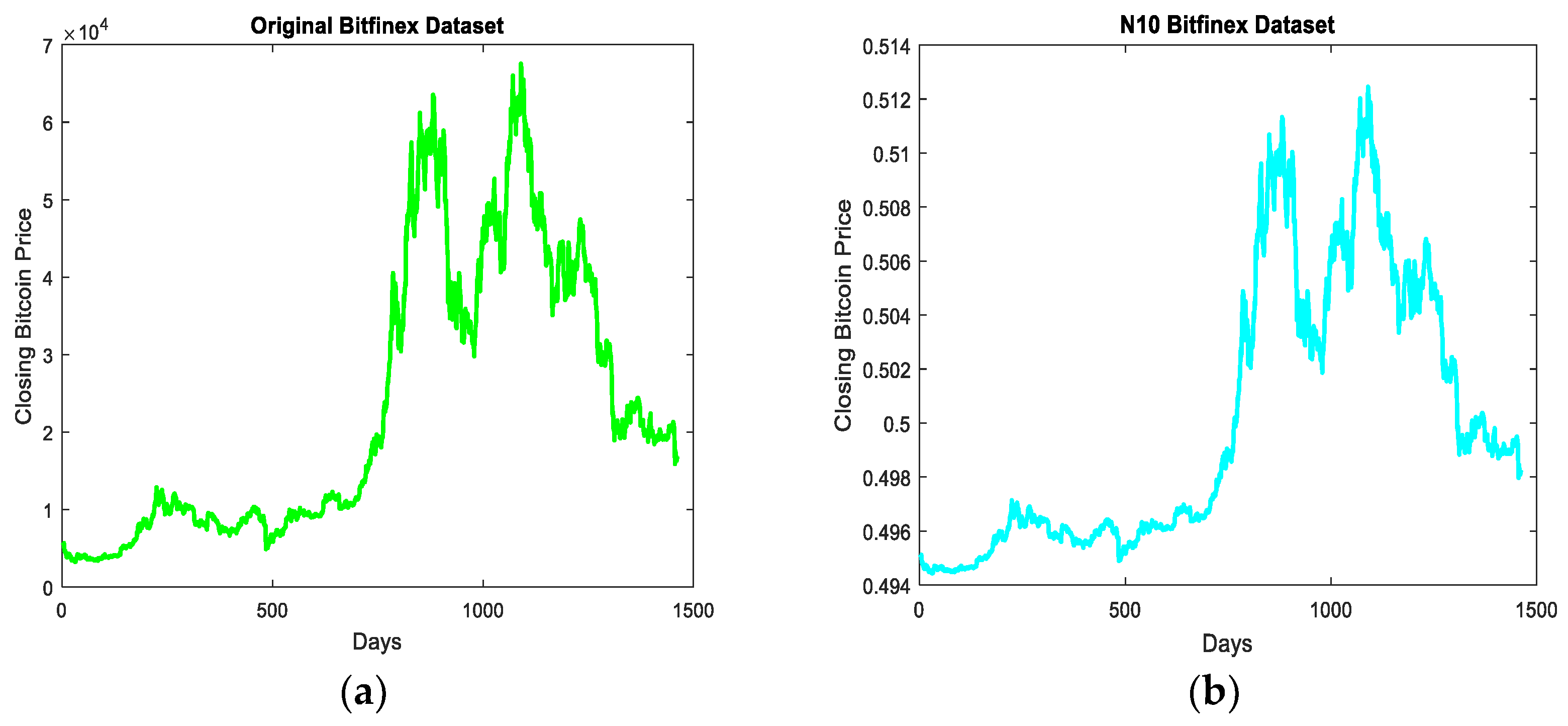
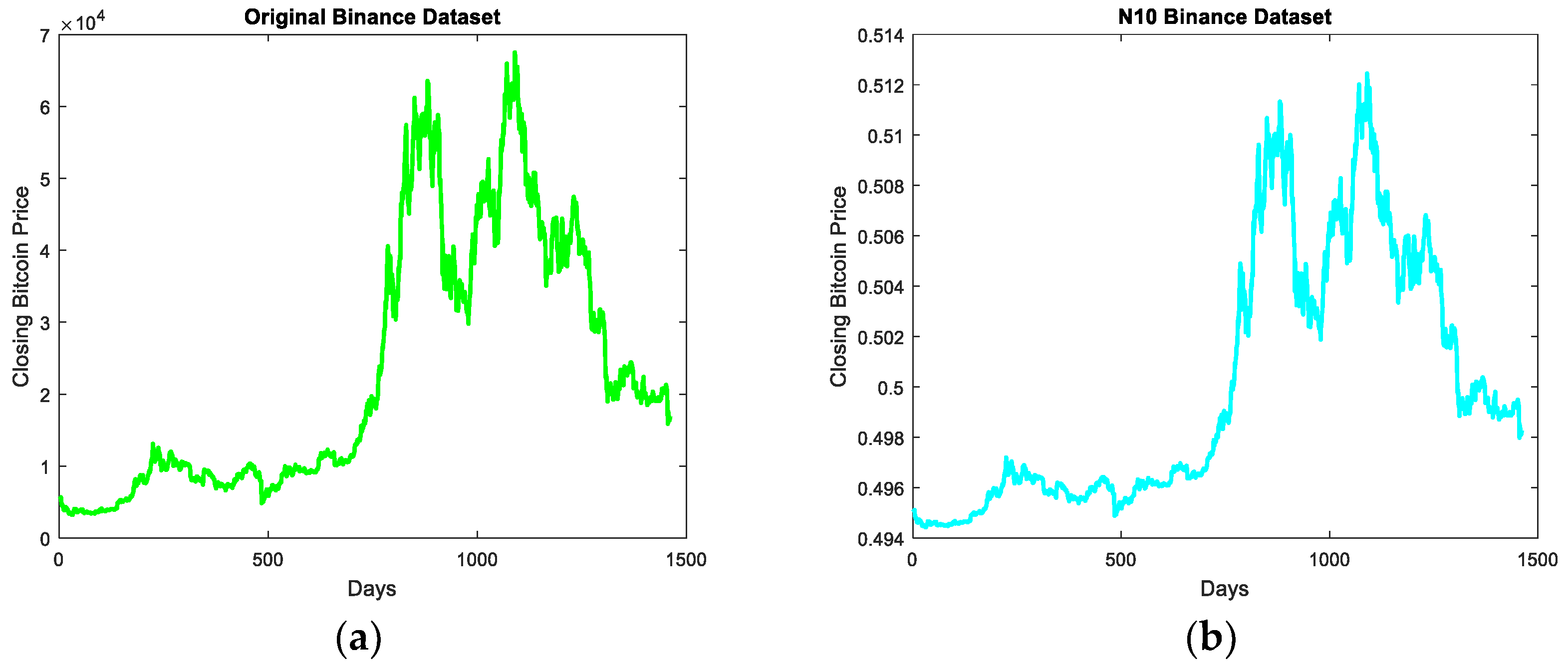
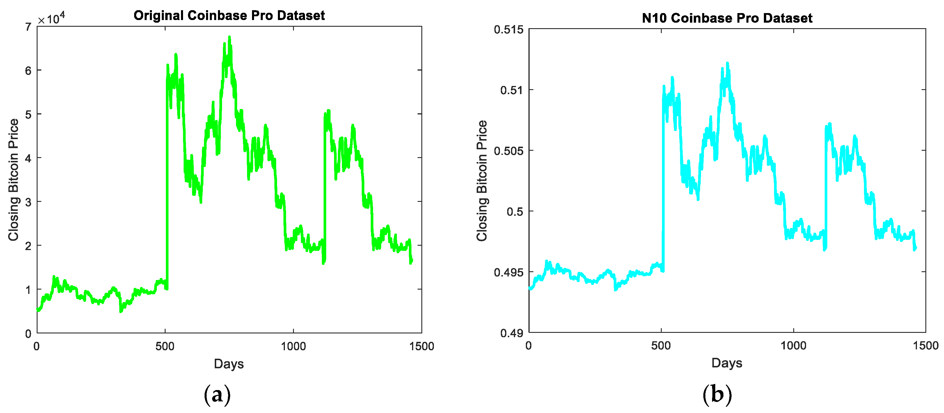
The stability of the proposed dual normalization technique was also tested by plotting the normalized dataset using dual normalization in all three datasets. The normalized plot along with the corresponding original dataset plot is presented in Figure 3, Figure 4 and Figure 5.
The proposed normalization was also analyzed by comparing the minimum and maximum values of each of the 10 normalizations under study. The normalized dataset analysis is presented in Table 5.
Table 5 indicates that the proposed normalization maps the value within the same range as other normalizations under study. All the normalization scales the values between 0 and 1.

4.5. Performance Evaluation

The new dual normalization method was used to generate a dataset for training and testing of the LMCMA model. The performance of the normalization methods was calculated by using 15 different error metrics, as shown in Table 6.
Out of the 15 error metrics, E5 is negatively oriented, and so a higher value is better. In contrast, the remaining 14 error measures are positively oriented.
After training, the performance of any single normalization method was not optimal. Some normalization gave better error values for certain error metrics but the worst values for some other metrics. So, a multi-criteria-based evaluation was made to find the top normalization methods.
The MCDM methods have been applied in many decision-making systems of organizations involving automobiles and airlines [55,56]. TOPSIS is an efficient and more accurate MCDM technique to rank various models under study [56,57]. Additionally, the TOPSIS ordering utilizes both best and worst criteria for picking the best model, and so it is highly reliable. TOPSIS was also proved to be better in terms of accuracy and robustness when applied to prediction and classification machine learning models [7,58,59]. Therefore, this study uses TOPSIS to select the best normalization in a FLANN network. TOPSIS analysis was used to rank the 16 models generated by using four normalizations (N1, N3, N7, N10) in Legendre FLANN (L1, L3, L7, L10), Chebyshev FLANN (C1, C3, C7, C10), Laguerre FLANN (La1, La3, La7, La10) and trigonometric FLANN (T1, T3, T7, T10).

5. Results

To test the second hypothesis this study, we divided each of the 10 normalized datasets into a train dataset and test dataset in a 2:1 ratio. A Legendre FLANN with 5 × 1 input–output neurons was used for training. The network used a sliding window of size 5 to input five historic prices and generate the 6th price. This model uses the RMSE value as a measure of fitness to be minimized by the MCMA algorithm. With a population of 20, this model is iterated 100 times to forecast the daily Bitcoin price for all the datasets. The optimized weights generated for each model under study are used to predict the test prices. The efficiency of each model was tested using 15 error measures. The minimum error metric was used as the final error after running each model 10 times.
The minimum error values for each normalization method in the testing of LMCMA model using the Bitfinex dataset are shown in Table 7.
From Table 7, it is observed that the N10-based model generated minimum values for error metrics E1, E2, E3, E4, E7, E8, E10, and E11. N2 gives optimal E5, E9, and E15. N3, N5, N8 and N9 give minimum E12, E6, E14, and E13, respectively.
The minimum error values for each normalization method in the testing of LMCMA model using the Binance dataset are shown in Table 8.
From Table 8, it is observed that the N10 based model generated minimum values for error metrics E1, E2, E3, E4, E7, E8, E10 and E11. N2 gives optimal values for E5 and E15. N4 gives minimum values for E6 and E13. N6 gives minimum values for E9, E12, and E14.
The minimum error values for each normalization method in the testing of LMCMA model using the Coinbase Pro dataset are shown in Table 9.
From Table 9, it is observed that the N10-based model generated minimum values for error metrics E1, E2, E4, E10, and E11. N3 gives minimum E12 and E13. N4 gives minimum E14 and E15. N6 gives minimum values for E9. N7 gives minimum values for E3, E7, and E8. N8 and N9 give optimal values for E5 and E6, respectively.
As it is visualized that none of the normalizations performs best for all error metrics, a TOPSIS-based ranking is conducted to rank the 10 normalization types during the testing of the LMCMA model. The ranking for each of the datasets under study is shown in Table 10, Table 11 and Table 12.
The ranking in all the three datasets indicates that normalization N10, N7, and N3 are the top three scalers in each of the datasets for the LMCMA model. To check the impact of our proposed normalization N10 on other networks, the original min–max normalization of LMCMA (N1) along with the top three ranked normalization (N10, N7, and N3) are used to test three other FLANNs.
The testing of four networks: Legendre FLANN (Network 1), Chebyshev FLANN (Network 2), Laguerre FLANN (Network 3), and trigonometric FLANN (Network 4) using four normalization types (N1, N3, N7, and N10) generate 16 MCMA-based Bitcoin predictor models: L1, L3, L7, L10, C1, C3, C7, C10, La1, La3, La7, La10, T1, T3, T7, and T10.
The value of 15 error metrics for 16 models under testing for the Bitfinex dataset is shown in Table 13.
Table 13 indicates that L10 minimizes E2, E3, E4, E7, E8, E10, and E11. L3 minimizes E13. C10 minimizes E1, E3, E4, and E10. La1 minimizes E6. T3 optimizes E5, E9, E12, and E15. T10 minimizes E1, E4, E10, and E14.
The value of 15 error metrics for 16 models under testing for the Binance dataset is shown in Table 14.
Table 14 indicates that C3 optimizes E5, E9, E14, and E15. C7 minimizes E3 and E10. T1 minimizes E6 and E13. T10 minimizes E1, E2, E3, E4, E7, E8, E10, E11, and E12.
The value of 15 error metrics for 16 models under testing for the Coinbase Pro dataset is shown in Table 14.
Table 15 indicates that L3 and L7 minimize E3 and E10. C1 minimizes E14. C3 optimizes E5 and E9. C10 minimizes E1, E3, E4, E7, E8, E10, E11, and E15. La1 minimizes E13. La7 minimizes E3. T1, T3, T7, and T10 minimize E6, E12, E2, and E3, respectively.
As none of the models under study dominated the performance, a TOPSIS-based ranking is executed for the three datasets. The ranking for the three datasets is shown in Table 16, Table 17 and Table 18.
Table 16 suggests that L10, C10, and T10 were the top three models in the Bitfinex dataset. The Binance dataset is best predicted by T10, C7, and C10 models as inferred from Table 17. Table 18 indicates that C10, L10, and L7 are the best predictor models for the Coinbase Pro dataset. The top three predictor models in each of the three datasets under study are represented in Table 19.
Table 19 indicates that the proposed dual normalization (N10) enhances the prediction capability of the FLANN networks under study.
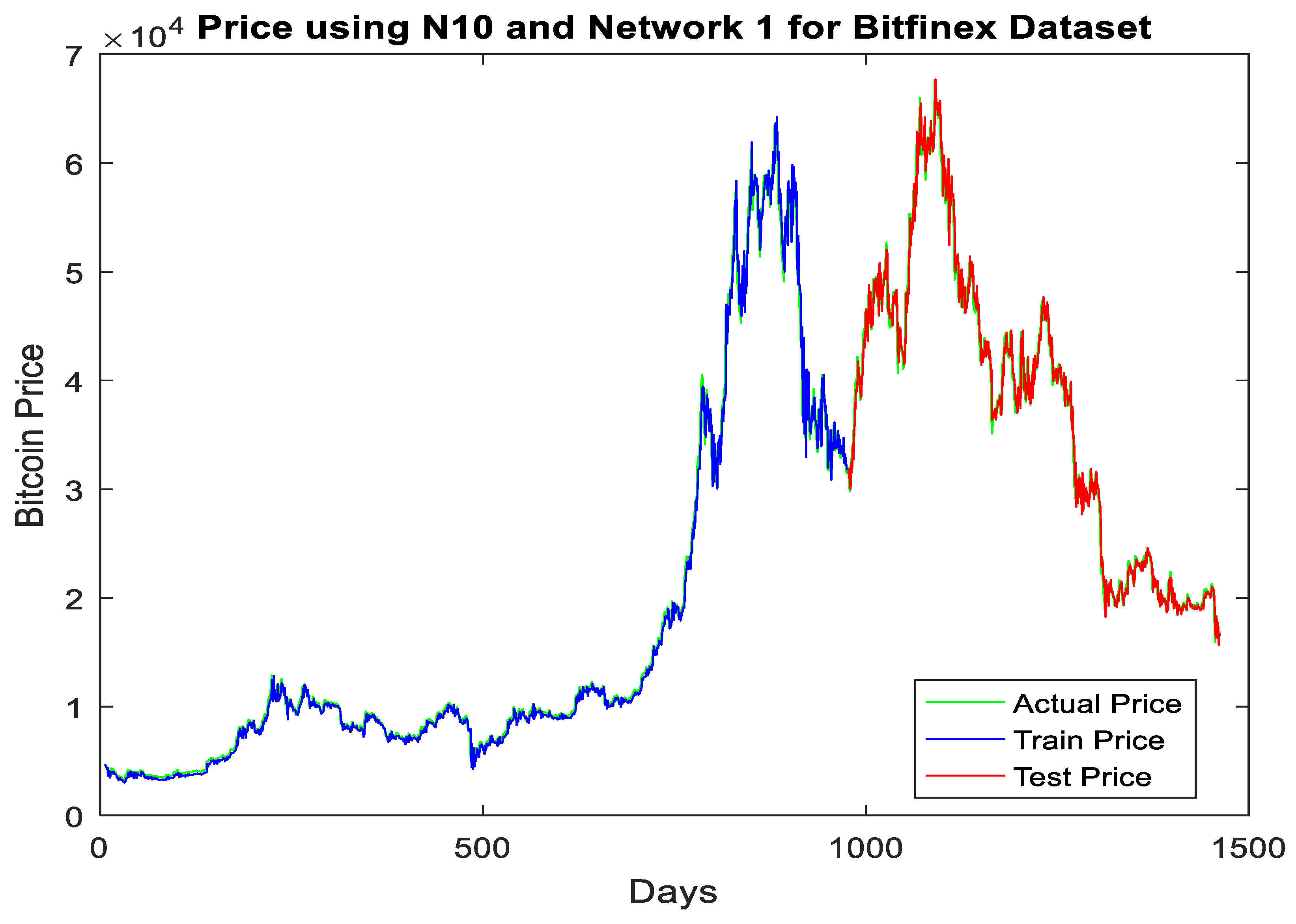
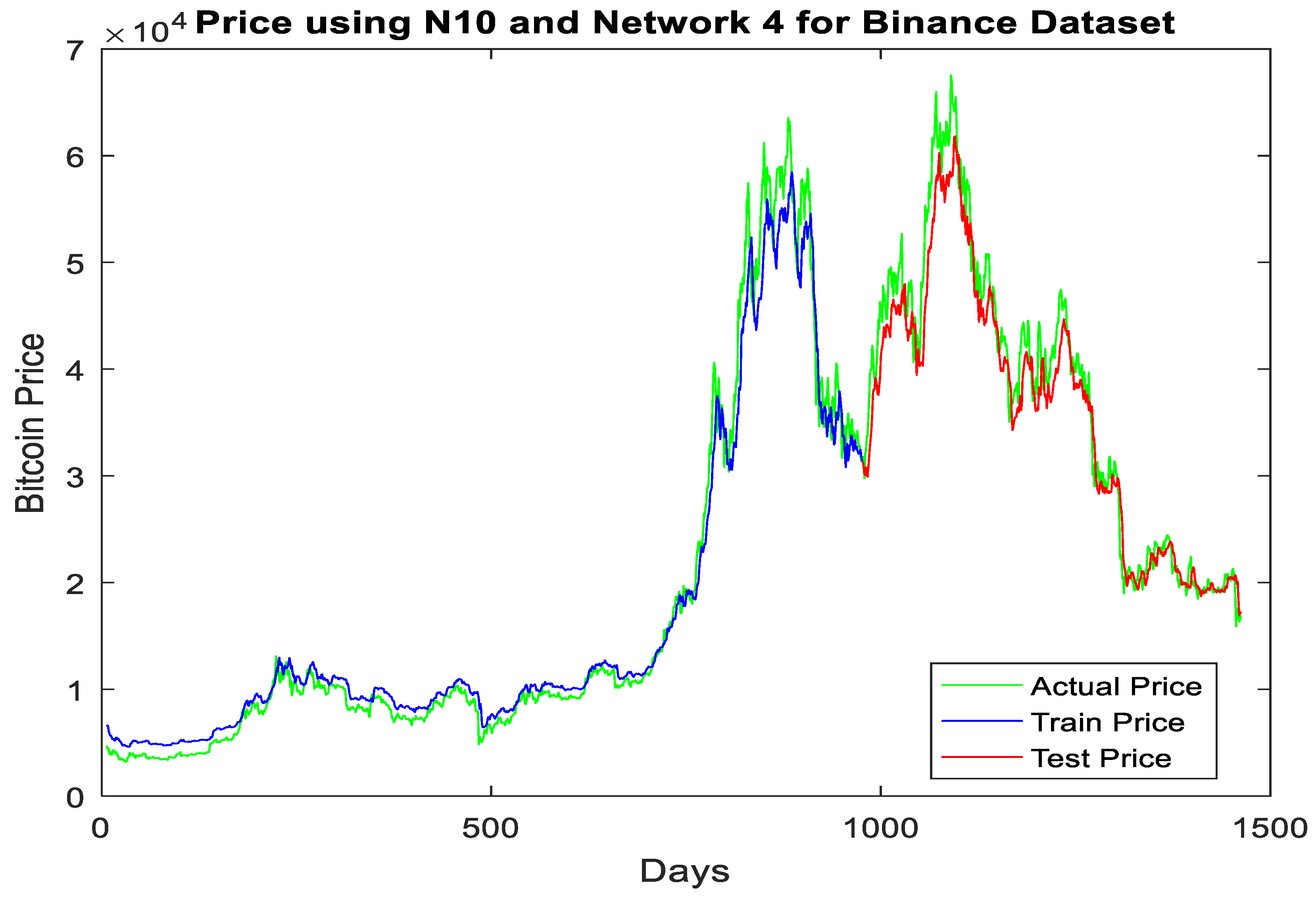
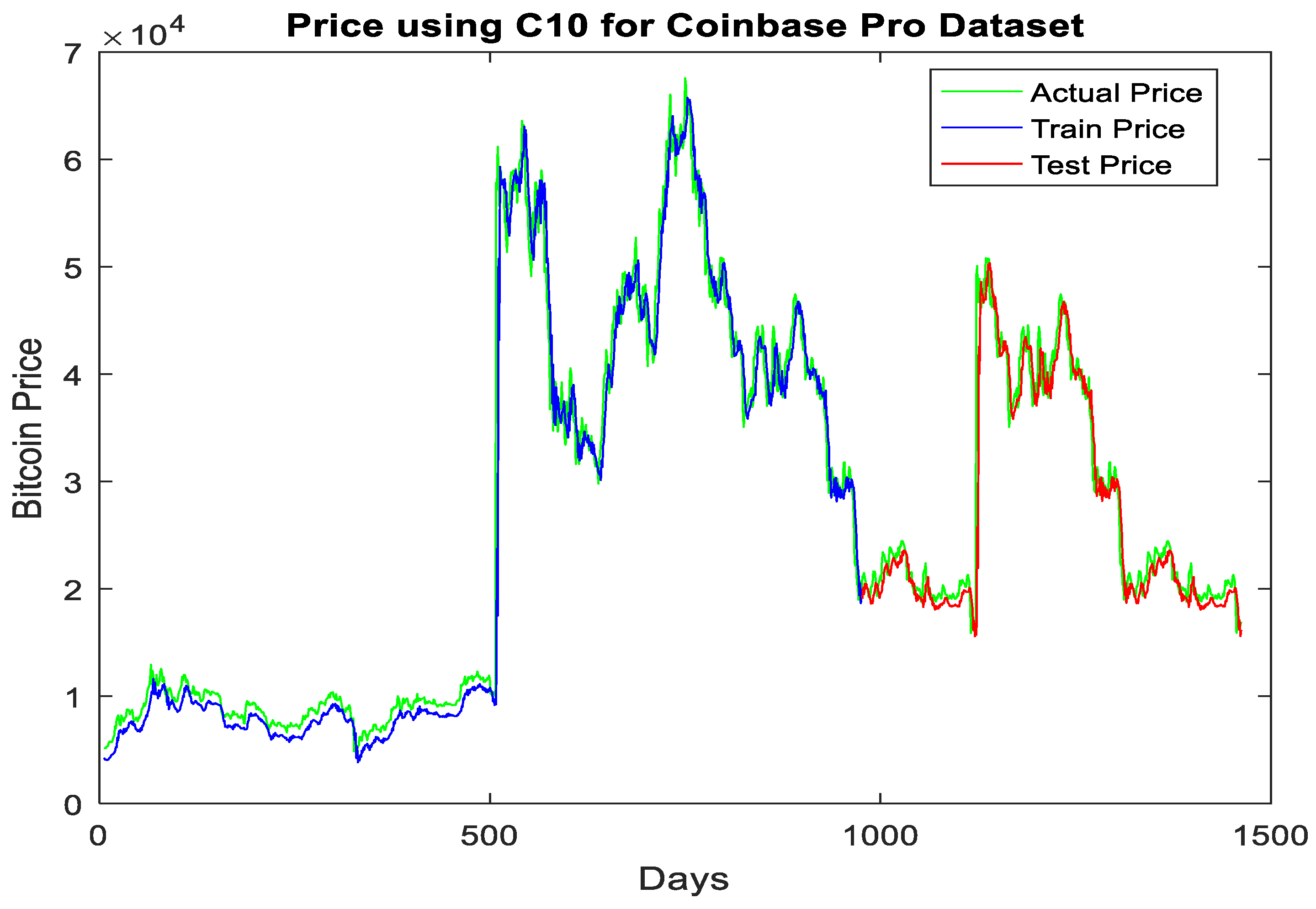
To present the mapping capability of the proposed normalization, the training, testing, and actual output of the first ranked model for each of the three datasets is shown in Figure 6, Figure 7 and Figure 8.
The mapping plots in Figure 6, Figure 7 and Figure 8 indicate that the dual normalization improves the prediction capability of polynomial-based neural network models. This validates the second hypothesis of this research.
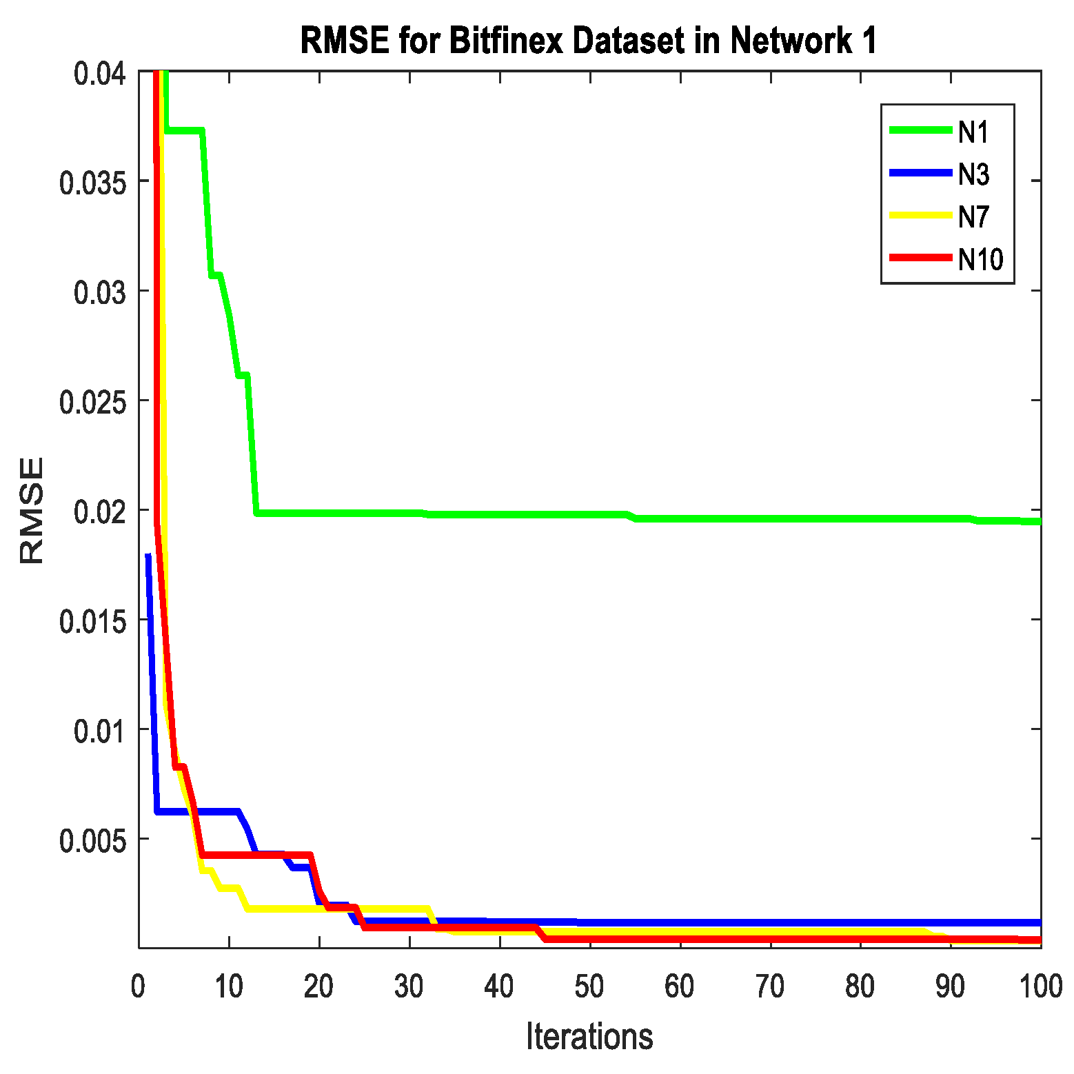
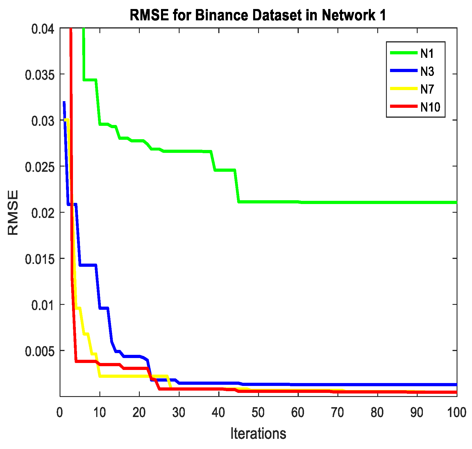
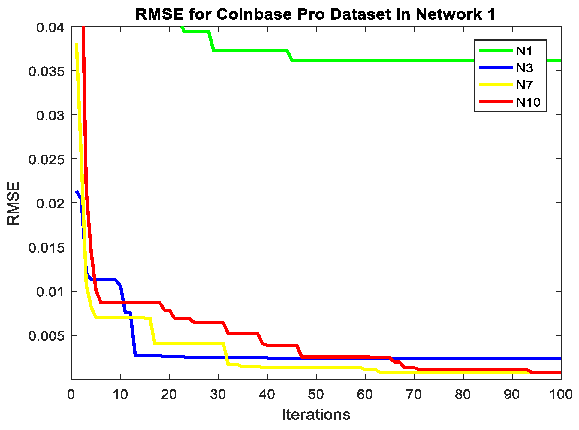
The convergence RMSE plot against the number of iterations for the training of the LMCMA model using N1, N3, N7, and the proposed N10 dataset for each of the three datasets is shown in Figure 9, Figure 10 and Figure 11.
The convergence plots in Figure 9, Figure 10 and Figure 11 clearly show that the proposed dual normalization minimizes the RMSE faster in comparison to other normalization under study. This also validates the second hypothesis of this study.
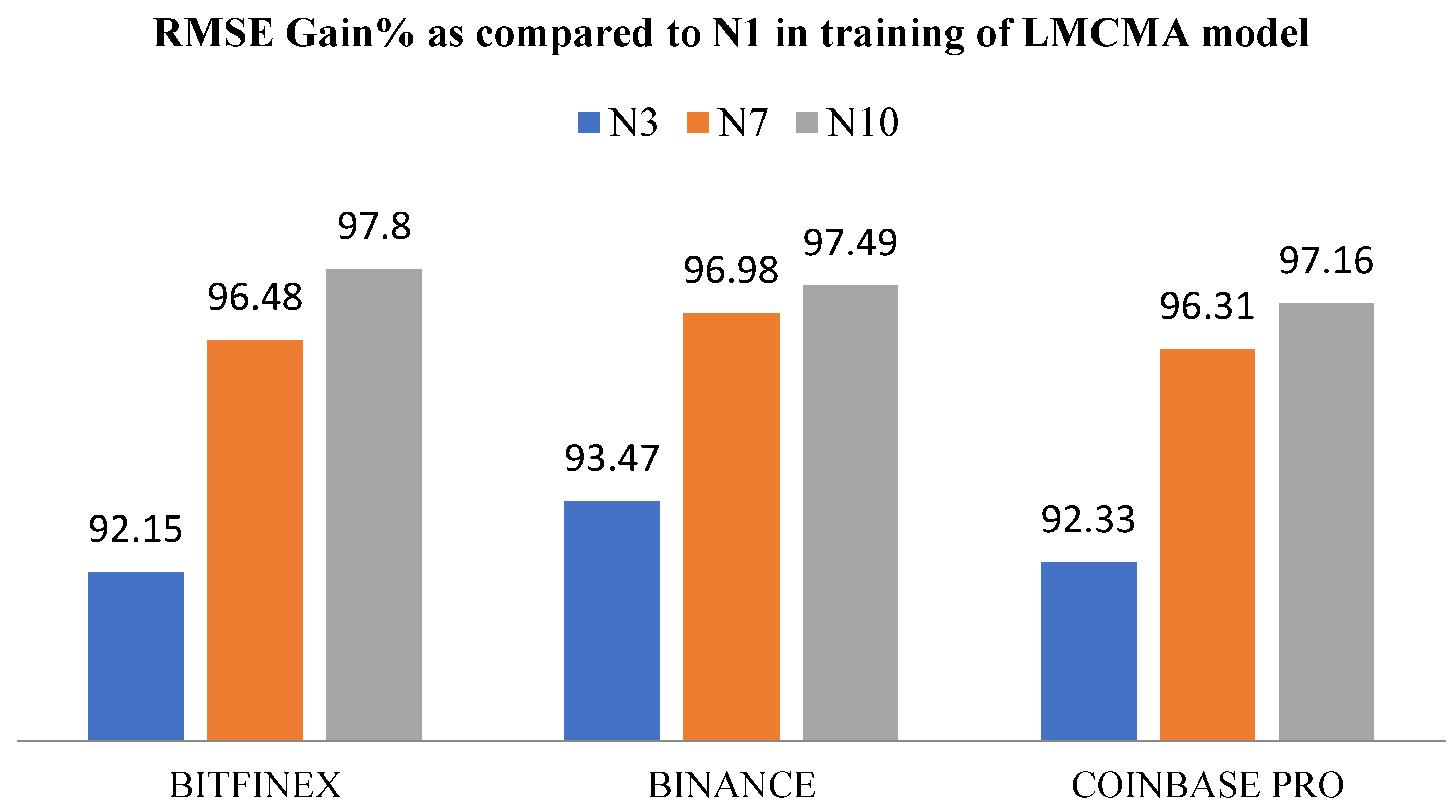
The RMSE gain percentage of the proposed normalization in comparison to the original min–max normalization used in the training of the LMCMA model is pictorially presented in Figure 12.
It is visualized in Figure 12 that the proposed dual normalization (N10) gives 97.8%, 97.49%, and 97.16% RMSE gain over the original min–max normalization (N1). It also shows that N10 predicts better than the basic N3 and N7 normalization used to generate the N10 technique.
The performance of the LMCMA model using the proposed dual normalization (L10) was further compared with two other models. The econometric Linear Regression (LR) model and the Support Vector Regression (SVR) model were used to predict the closing Bitcoin prices on the three datasets under study. The error measures for test data are presented in Table 20.
As observed in Table 20, the L10 model performs better than the LR and the SVR model in terms of all the error measures. The RMSE of each of the three models for the three datasets under study is shown in Figure 13.
As observed from Figure 13, the LMCMA model using the proposed dual normalization (N10) outperformed the LR and SVR models.
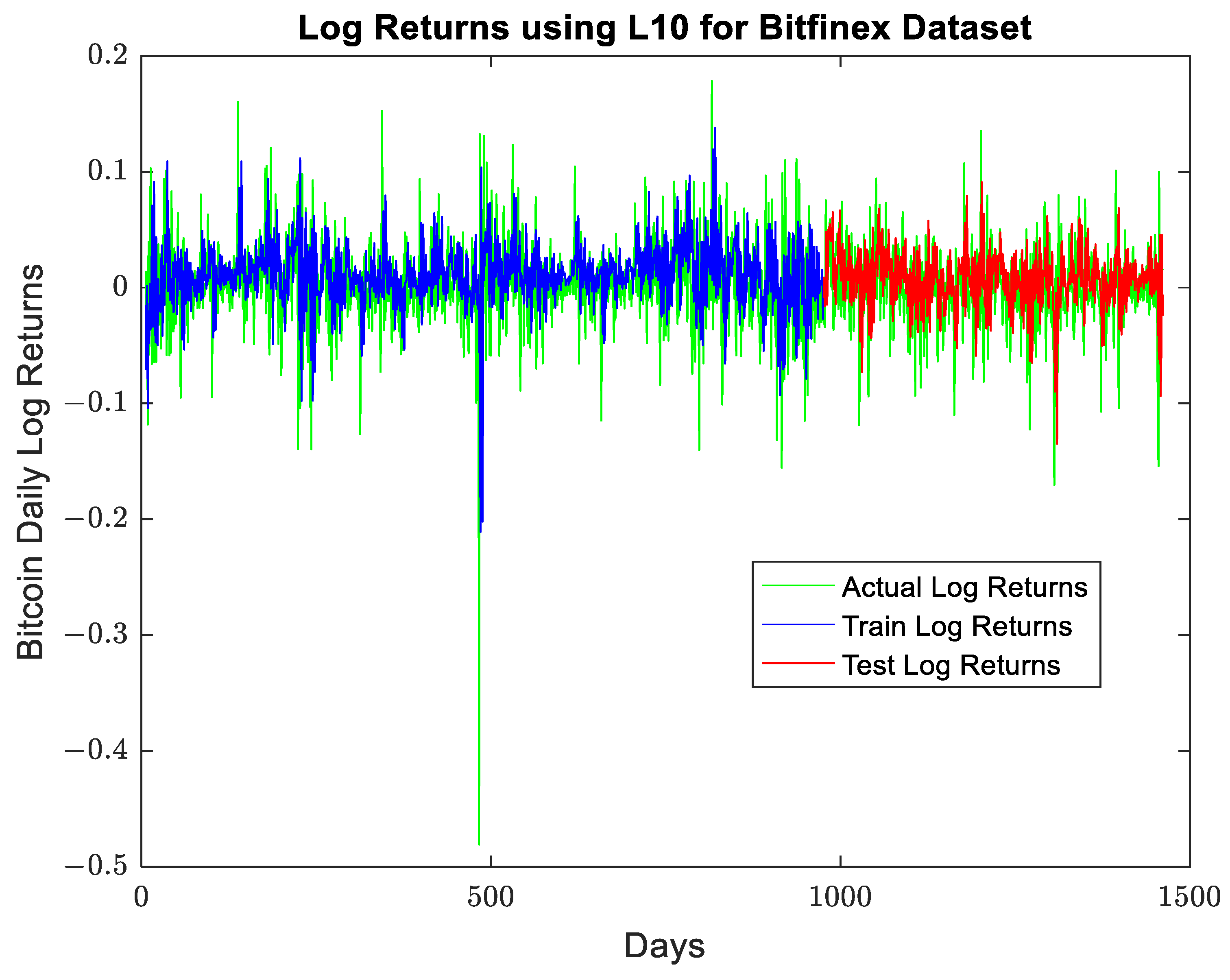
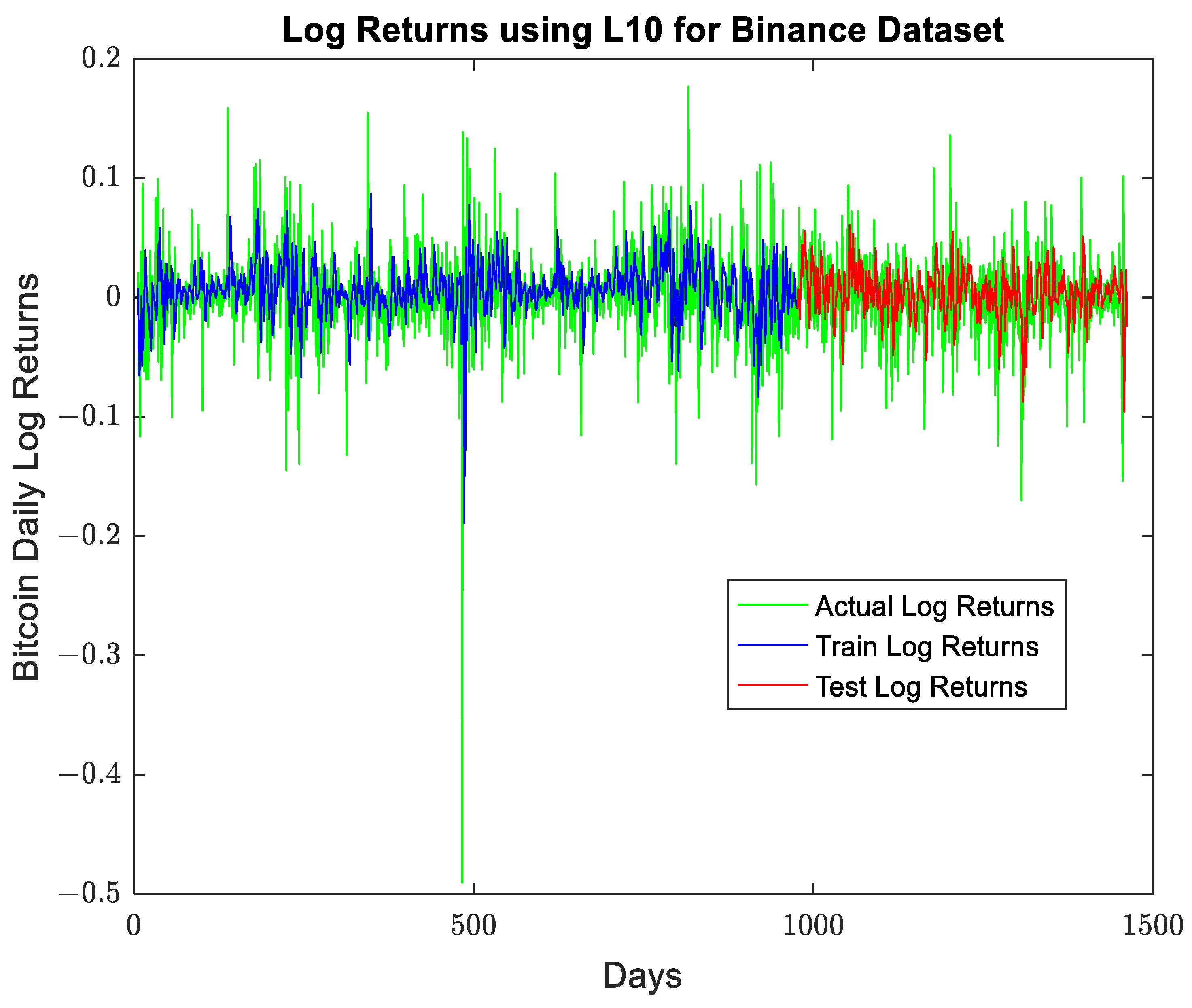
The Bitcoin closing prices are highly volatile, and as logarithmic distribution is more normal as compared to raw prices, this study further analyzed the performance of the proposed dual normalization on Bitcoin log returns for the three datasets under study. The error measures for each dataset are presented in Table 21.
As indicated by Table 21, the LMCMA model using the new normalization technique gives an RMSE of 0.0051, 0.0053, and 0.0052 for the Bitfinex, Binance, and Coinbase Pro datasets, respectively. In addition, the model performs well in all three datasets. The actual Bitcoin log returns plotted against the predicted train and test log returns for all the three datasets are shown in Figure 14, Figure 15 and Figure 16.

6. Discussion

Recently, Bitcoin is assumed to be a safe-haven asset by some investors. However, the dynamic and volatile behavior of the Bitcoin dataset is the biggest challenge to the growth of the Bitcoin market. A Bitcoin predictor model with sufficient stability can act as fuel in increasing investors and stakeholders in the digital market. The emergence of Bitcoin Cash has already created a positive spur in the digitization of companies [60]. Many research activities are involved in analyzing the Bitcoin dataset to suggest a better model of regression or classification.
In this study, the Bitcoin prices of three different markets were normalized using different normalization types and were analyzed in the LMCMA model to obtain the top normalization for pricing. A dual normalization was proposed using the top two normalizations during the training of the LMCMA model. The stability of the normalization technique proposed here is validated by testing its efficiency in a different test dataset. Additionally, the top performers were evaluated in three other FLANN models. As the performance evaluation of these 16 models is not decisive, this study utilized the TOPSIS-based performance measurement with 15 errors. The proposed normalization bagged the first rank in each of the datasets.
As the datasets were divided into training and testing datasets which have no common data between them, the efficient prediction of the proposed normalization during testing and training of the FLANN models suggest the stable feature of this normalization. It can be visualized in Table 14, Table 15 and Table 16 that the proposed normalization (N10) performs best in each network separately for all the three datasets.
In the Bitfinex dataset, Legendre-based models L1, L3, L7, and L10 were ranked 13, 12, 7, and 1, respectively. Similarly, Chebyshev models C1, C3, C7, and C10 were ranked 14, 9, 4, and 2, respectively. Laguerre models La1, La3, La7, and La10 were ranked 16, 11, 10, and 8, respectively. Trigonometric models T1, T3, T7, and T10 were ranked 15, 6, 5, and 3, respectively. It indicates that N10 outperformed the other normalization techniques in each of the networks. The similar inference is also validated for Binance and Coinbase Pro datasets. This also validates the stability of the proposed normalization.
As inferred from Table 19, although N10 is the best normalization in each network, still, the overall model for best prediction is different for different datasets. So, the network architecture also plays a vital role in the modeling of predictors.
The output plots for the first ranked model in each dataset clearly show the efficient mapping of dual normalization in Bitcoin price prediction. Furthermore, the RMSE gain percent of N10 during training is 97.8%, 97.49%, and 97.16% for Bitfinex, Binance, and Coinbase Pro datasets, respectively. The RMSE gain percentage for testing is 81.37%, 98.13%, and 98.73% for Bitfinex, Binance, and Coinbase Pro datasets, respectively.
The novelty of the proposed dual normalization is compared with some hybrid normalization available in the literature. It is shown in Table 22.
Table 22 suggests that our proposed dual normalization is novel and efficient work in the field of Bitcoin price prediction. It is more reliable, as it is evaluated using 15 error metrics. This normalization is also stable as data can be denormalized to actual ones for better mapping.
This study also compared the linear regression econometric model with the proposed model. The nonlinear regression SVR is also analyzed and compared to the L10 model. The results indicate that the proposed model is efficient for Bitcoin price prediction. Similar results were also observed in predicting the Bitcoin daily log returns. The highly volatile feature of Bitcoin price is also mapped efficiently by the predictor model L10.

7. Conclusions

Recently, Bitcoin has been dominating the crypto market. This paper proposes a new dual normalization technique to efficiently predict Bitcoin closing prices by handling the huge variations in the dataset. This is the first paper to study the impact of data scaling on Bitcoin prices. To validate the proposed normalization, it was compared with nine different normalizations applied to three different datasets for modeling four different FLANNs. Furthermore, the predicted and actual outputs were plotted. The mapping of outputs visualizes the efficiency of the proposed method. To further validate the dataset, distribution plots are used. The use of this normalization enhances the prediction capability of the LMCMA model by giving an RMSE gain percent of more than 90 over min–max normalization in the Bitfinex, Binance, and Coinbase Pro datasets.
This research can help many investors and stakeholders in the crypto-market to make appropriate decisions on Bitcoin pricing. In addition, the proposed normalization indicates that instead of having a fixed normalization for research, different normalizations can be analyzed to select the best normalization for a particular network. This can give research directions to any area of research which requires normalization of its input.
During COVID-19, the huge rise in Bitcoin prices prompted many investors to invest in the crypto-market. However, after the pandemic, the decline in Bitcoin prices left many investors in dismay. The Bitcoin price is highly volatile and is in its initial phase. So, many econometric models need to be evaluated along with the FLANN-based model, which provides higher accuracy. However, this study reveals that an appropriate normalization can help in better scaling of such huge volatility in Bitcoin prices. This in turn can help in positive decisions with profitable investment in the crypto-market.
Although this study presented a novel idea to analyze normalization before any regression or classification, it has a few shortcomings which can be addressed in the future. The new normalization has only been tested on FLANN models, a linear regression model, and a nonlinear SVR model. It can be further tested for different other networks and econometric models. Additionally, this normalization can be tested for several other datasets to explore its capability in different areas of research. The models can be fine-tuned further by using several other machine-learning algorithms. A close look at the normalized data analysis points out that the range of transformation may play a vital role in the efficiency of a model. This needs to be further analyzed. This model analyzes the prediction of the closing prices, which is not sufficient to address the high volatility. In addition, the log returns prediction needs to be analyzed for different other networks for a better prediction It can be further used to normalize technical indicators and combine them with normalization types. As Bitcoin is highly volatile, its price movement prediction needs to be explored. The effect of different other preprocessing techniques such as window size and the ratio of splitting the dataset can be analyzed in the future. Furthermore, this research can be extended by designing an econometric model using various technical, social, and economic indicators which may influence the Bitcoin price volatility.

Author Contributions

Conceptualization, S.M. and R.D.; methodology, S.M.; software, S.M.; validation, S.M. and R.D.; formal analysis, S.M.; investigation, S.M.; resources, S.M.; data curation, S.M.; writing—original draft preparation, S.M.; writing—review and editing, S.M.; visualization, S.M.; supervision, R.D.; project administration, R.D.; funding acquisition, S.M. All authors have read and agreed to the published version of the manuscript.

Funding

This research received no external funding.

Data Availability Statement

Publicly available datasets were analyzed in this study. These data can be found here: http://www.investing.com/crypto/bitcoin/historical-data, accessed on 15 November 2022.

Conflicts of Interest

The authors declare no conflict of interest.

References

  1. Steinmetz, F.; von Meduna, M.; Ante, L.; Fiedler, I. Ownership, Uses and Perceptions of Cryptocurrency: Results from a Population Survey. Technol. Forecast. Soc. Change 2021, 173, 121073. [Google Scholar] [CrossRef]
  2. Sai, A.R.; Buckley, J.; Fitzgerald, B.; Gear, A.L. Taxonomy of Centralization in Public Blockchain Systems: A Systematic Literature Review. Inf. Process. Manag. 2021, 58, 102584. [Google Scholar] [CrossRef]
  3. Selgin, G. Synthetic Commodity Money. J. Fin. Stab. 2015, 17, 92–99. [Google Scholar] [CrossRef]
  4. Nayak, S.C. Bitcoin Closing Price Movement Prediction with Optimal Functional Link Neural Networks. Evol. Intell. 2022, 15, 1825–1839. [Google Scholar] [CrossRef]
  5. Kim, G.; Shin, D.-H.; Choi, J.G.; Lim, S. A Deep Learning-Based Cryptocurrency Price Prediction Model That Uses on-Chain Data. IEEE Access 2022, 10, 56232–56248. [Google Scholar] [CrossRef]
  6. Pour, E.S.; Jafari, H.; Lashgari, A.; Rabiee, E.; Ahmadisharaf, A. Cryptocurrency Price Prediction with Neural Networks of LSTM and Bayesian Optimization. Eur. J. Bus. Manag. Res. 2022, 7, 20–27. [Google Scholar] [CrossRef]
  7. Mohanty, S.; Dash, R. Neural Network-Based Bitcoin Pricing Using a New Mutated Climb Monkey Algorithm with TOPSIS Analysis for Sustainable Development. Mathematics 2022, 10, 4370. [Google Scholar] [CrossRef]
  8. Basher, S.A.; Sadorsky, P. Forecasting Bitcoin Price Direction with Random Forests: How Important Are Interest Rates, Inflation, and Market Volatility? Mach. Learn. Appl. 2022, 9, 100355. [Google Scholar] [CrossRef]
  9. Erfanian, S.; Zhou, Y.; Razzaq, A.; Abbas, A.; Safeer, A.A.; Li, T. Predicting Bitcoin (BTC) Price in the Context of Economic Theories: A Machine Learning Approach. Entropy 2022, 24, 1487. [Google Scholar] [CrossRef]
  10. Rathore, R.K.; Mishra, D.; Mehra, P.S.; Pal, O.; Hashim, A.S.; Shapi’i, A.; Ciano, T.; Shutaywi, M. Real-World Model for Bitcoin Price Prediction. Inf. Process. Manag. 2022, 59, 102968. [Google Scholar] [CrossRef]
  11. Huang, J.-Z.; Huang, W.; Ni, J. Predicting Bitcoin Returns Using High-Dimensional Technical Indicators. J. Financ. Data Sci. 2019, 5, 140–155. [Google Scholar] [CrossRef]
  12. Mallqui, D.C.A.; Fernandes, R.A.S. Predicting the Direction, Maximum, Minimum and Closing Prices of Daily Bitcoin Exchange Rate Using Machine Learning Techniques. Appl. Soft Comput. 2019, 75, 596–606. [Google Scholar] [CrossRef]
  13. Rajabi, S.; Roozkhosh, P.; Farimani, N.M. MLP-Based Learnable Window Size for Bitcoin Price Prediction. Appl. Soft Comput. 2022, 129, 109584. [Google Scholar] [CrossRef]
  14. Shanker, M.; Hu, M.Y.; Hung, M.S. Effect of Data Standardization on Neural Network Training. Omega 1996, 24, 385–397. [Google Scholar] [CrossRef]
  15. Ahsan, M.; Mahmud, M.; Saha, P.; Gupta, K.; Siddique, Z. Effect of Data Scaling Methods on Machine Learning Algorithms and Model Performance. Technologies 2021, 9, 52. [Google Scholar] [CrossRef]
  16. Singh, D.; Singh, B. Investigating the Impact of Data Normalization on Classification Performance. Appl. Soft Comput. 2020, 97, 105524. [Google Scholar] [CrossRef]
  17. Nayak, S.C.; Misra, B.B.; Behera, H.S. Impact of Data Normalization on Stock Index Forecasting. Int. J. Comput. Inf. Syst. Ind. Manag. Appl. 2014, 6, 257–269. [Google Scholar]
  18. Pan, J.; Zhuang, Y.; Fong, S. The Impact of Data Normalization on Stock Market Prediction: Using SVM and Technical Indicators. In International Conference on Soft Computing in Data Science; Springer: Singapore, 2016; pp. 72–88. [Google Scholar]
  19. Peng, Y.; Albuquerque, P.H.; Camboium de Sá, J.M.; Padula, A.J.; Montenegro, M.R. The Best of Two Worlds: Forecasting High Frequency Volatility for Cryptocurrencies and Traditional Currencies with Support Vector Regression. Expert Syst. Appl. 2018, 97, 177–192. [Google Scholar] [CrossRef]
  20. Aggarwal, D.; Chandrasekaran, S.; Annamalai, B. A Complete Empirical Ensemble Mode Decomposition and Support Vector Machine-Based Approach to Predict Bitcoin Prices. J. Behav. Exp. Financ. 2020, 27, 100335. [Google Scholar] [CrossRef]
  21. Liu, M.; Li, G.; Li, J.; Zhu, X.; Yao, Y. Forecasting the price of Bitcoin using deep learning. Finance Res. Lett. 2021, 40, 101755. [Google Scholar] [CrossRef]
  22. Nayak, S.C.; Misra, B.B.; Dehuri, S. Hybridization of the Higher Order Neural Networks with the Evolutionary Optimization Algorithms-An Application to Financial Time Series Forecasting. In Advances in Machine Learning for Big Data Analysis; Springer: Singapore, 2022; pp. 119–144. [Google Scholar]
  23. Ye, J.; Xie, L.; Ma, L.; Bian, Y.; Xu, X. A Novel Hybrid Model Based on Laguerre Polynomial and Multi-Objective Runge–Kutta Algorithm for Wind Power Forecasting. Int. J. Electr. Power Energy Syst. 2023, 146, 108726. [Google Scholar] [CrossRef]
  24. Dash, R. DECPNN: A Hybrid Stock Predictor Model Using Differential Evolution and Chebyshev Polynomial Neural Network. Intell. Decis. Technol. 2018, 12, 93–104. [Google Scholar] [CrossRef]
  25. Mohanty, S.; Dash, R. Predicting the Price of Gold: A CSPNN-DE Model. In Intelligent and Cloud Computing; Springer: Singapore, 2021; pp. 289–297. [Google Scholar]
  26. Mohanty, S.; Dash, R. A Novel Chaotic Flower Pollination Algorithm for Modelling an Optimized Low-Complexity Neural Network-Based NAV Predictor Model. Prog. Artif. Intell. 2022, 11, 349–366. [Google Scholar] [CrossRef]
  27. Nayak, S.C.; Misra, B.B.; Behera, H.S. Comparison of Performance of Different Functions in Functional Link Artificial Neural Network: A Case Study on Stock Index Forecasting. In Computational Intelligence in Data Mining—Volume 1; Springer: New Delhi, India, 2015; pp. 479–487. [Google Scholar]
  28. Das, S.; Nayak, S.C.; Sahoo, B. Towards Crafting Optimal Functional Link Artificial Neural Networks with Rao Algorithms for Stock Closing Prices Prediction. Comput. Econ. 2022, 60, 1–23. [Google Scholar] [CrossRef]
  29. Dash, R.; Dash, P.K. Stock Price Index Movement Classification Using a CEFLANN with Extreme Learning Machine. In Proceedings of the 2015 IEEE Power, Communication and Information Technology Conference 2015 (PCITC), Bhubaneswar, India, 15–17 October 2015. [Google Scholar]
  30. Jain, S.; Shukla, S.; Wadhvani, R. Dynamic Selection of Normalization Techniques Using Data Complexity Measures. Expert Syst. Appl. 2018, 106, 252–262. [Google Scholar] [CrossRef]
  31. Friedman, M. AComparison of Alternative Tests of Significance for the Problem of m Rankings. Ann. Math. Stat. 1940, 11, 86–92. [Google Scholar] [CrossRef]
  32. Alshdaifat, E.; Alshdaifat, D.; Alsarhan, A.; Hussein, F.; El-Salhi, S.M.F.S. The Effect of Preprocessing Techniques, Applied to Numeric Features, on Classification Algorithms’ Performance. Data 2021, 6, 11. [Google Scholar] [CrossRef]
  33. Nemenyi, P.B. Distribution-Free Multiple Comparisons. Ph.D. Thesis, Princeton University, Princeton, UK, 1963. [Google Scholar]
  34. Singh, D.; Singh, B. Feature Wise Normalization: An Effective Way of Normalizing Data. Pattern Recognit. 2022, 122, 108307. [Google Scholar] [CrossRef]
  35. Sola, J.; Sevilla, J. Importance of Input Data Normalization for the Application of Neural Networks to Complex Industrial Problems. IEEE Trans. Nucl. Sci. 1997, 44, 1464–1468. [Google Scholar] [CrossRef]
  36. Dębkowska, K.; Jarocka, M. The Impact of the Methods of the Data Normalization on the Result of Linear Ordering. Acta Univ. Lodz. Folia Oeconomica 2013, 286, 181–198. [Google Scholar]
  37. Cakir, L.; Konakoglu, B. The impact of data normalization on 2D coordinate transformation using GRNN. Geod. Vestn. 2019, 63, 541–553. [Google Scholar] [CrossRef]
  38. Vafaei, N.; Ribeiro, R.A.; Camarinha-Matos, L.M. Normalization Techniques for Multi-Criteria Decision Making: Analytical Hierarchy Process Case Study. In Technological Innovation for Cyber-Physical Systems; Springer International Publishing: Cham, Switzerland, 2016; pp. 261–269. [Google Scholar]
  39. Aytekin, A. Comparative Analysis of the Normalization Techniques in the Context of MCDM Problems. Decis. Mak. Appl. Manag. Eng. 2021, 4, 1–25. [Google Scholar] [CrossRef]
  40. Chakraborty, S.; Yeh, C.H. A Simulation Based Comparative Study of Normalization Procedures in Multiattribute Decision Making. In Proceedings of the 6th Conference on 6th WSEAS Int. Conf. on Artificial Intelligence, Knowledge Engineering and Data Bases, Corfu Island, Greece, 16–19 February 2007; Volume 6, pp. 102–109. [Google Scholar]
  41. Jahan, A.; Edwards, K.L. A State-of-the-Art Survey on the Influence of Normalization Techniques in Ranking: Improving the Materials Selection Process in Engineering Design. Mater. Eng. 2015, 65, 335–342. [Google Scholar] [CrossRef]
  42. Chakraborty, S.; Yeh, C.-H. A Simulation Comparison of Normalization Procedures for TOPSIS. In Proceedings of the 2009 International Conference on Computers & Industrial Engineering, Troyes, France, 6–9 July 2009. [Google Scholar]
  43. Kumari, B.; Swarnkar, T. Stock Movement Prediction Using Hybrid Normalization Technique and Artificial Neural Network. Int. J. Adv. Technol. Eng. Explor. 2021, 8, 1336. [Google Scholar] [CrossRef]
  44. Izonin, I.; Tkachenko, R.; Shakhovska, N.; Ilchyshyn, B.; Singh, K.K. A Two-Step Data Normalization Approach for Improving Classification Accuracy in the Medical Diagnosis Domain. Mathematics 2022, 10, 1942. [Google Scholar] [CrossRef]
  45. Batrancea, L. The Influence of Liquidity and Solvency on Performance within the Healthcare Industry: Evidence from Publicly Listed Companies. Mathematics 2021, 9, 2231. [Google Scholar] [CrossRef]
  46. Batrancea, L.M. An Econometric Approach on Performance, Assets, and Liabilities in a Sample of Banks from Europe, Israel, United States of America, and Canada. Mathematics 2021, 9, 3178. [Google Scholar] [CrossRef]
  47. Reverter, A.; Barris, W.; McWilliam, S.; Byrne, K.A.; Wang, Y.H.; Tan, S.H.; Hudson, N.; Dalrymple, B.P. Validation of alternative methods of data normalization in gene co-expression studies. Bioinformatics 2019, 21, 1112–1120. [Google Scholar] [CrossRef] [Green Version]
  48. Han, J.; Kamber, M.; Pei, J. Data Mining: Concepts and Techniques; Morgan Kaufmann: Oxford, UK, 2012. [Google Scholar]
  49. Brauers, W.K.; Zavadskas, E.K. The MOORA Method and Its Application to Privatization in a Transition Economy. Control. Cybern. 2006, 35, 445–469. [Google Scholar]
  50. Chen, C.; Kitbutrawat, N.; Kajita, S.; Yamaguchi, H.; Higashino, T. Modeling BLE Propagation Above the Ceiling for Smart HVAC Systems. In Proceedings of the 2019 15th International Conference on Intelligent Environments (IE), Rabat, Morocco, 24–27 June 2019; pp. 68–71. [Google Scholar]
  51. Gardziejczyk, W.; Zabicki, P. Normalization and Variant Assessment Methods in Selection of Road Alignment Variants- Case Study. J. Civ. Eng. Manag. 2017, 23, 510–523. [Google Scholar] [CrossRef]
  52. Rousseeuw, P.J.; Hampel, F.R.; Ronchetti, E.M.; Stahel, W.A. Robust Statistics: The Approach Based on Influence Functions; John Wiley & Sons: Hoboken, NJ, USA, 2011. [Google Scholar]
  53. Theodoridis, S.; Koutroumbas, K.; Pikrakis, A.; Cavouras, D. Introduction to Pattern Recognition: A MATLAB Approach; Academic Press: Cambridge, MA, USA, 2010. [Google Scholar]
  54. Jayalakshmi, T.; Santhakumaran, A. Statistical Normalization and Back Propagationfor Classification. Int. J. Comput. Theory Eng. 2011, 3, 89–93. [Google Scholar] [CrossRef]
  55. Cocis, A.-D.; Batrancea, L.; Tulai, H. The link between corporate reputation and financial performance and equilibrium within the airline industry. Mathematics 2021, 9, 2150. [Google Scholar] [CrossRef]
  56. Batrancea, L.M.; Nichita, A.; Cocis, A.-D. Financial performance and sustainable corporate reputation: Empirical evidence from the airline business. Sustainability 2022, 14, 13567. [Google Scholar] [CrossRef]
  57. Samal, S.; Dash, R. A TOPSIS-ELM Framework for Stock Index Price Movement Prediction. Intell. Decis. Technol. 2021, 15, 201–220. [Google Scholar] [CrossRef]
  58. Dash, R.; Samal, S.; Dash, R.; Rautray, R. An Integrated TOPSIS Crow Search Based Classifier Ensemble: In Application to Stock Index Price Movement Prediction. Appl. Soft Comput. 2019, 85, 105784. [Google Scholar] [CrossRef]
  59. Samal, S.; Dash, R. Developing a Novel Stock Index Trend Predictor Model by Integrating Multiple Criteria Decision-Making with an Optimized Online Sequential Extreme Learning Machine. Granul. Comput. 2022. [Google Scholar] [CrossRef]
  60. Hossain, S.A. Blockchain computing: Prospects and challenges for digital transformation. In Proceedings of the 6th International Conference on Reliability, Infocom Technologies and Optimization (Trends and Future Directions), Noida, India, 20–22 September2017; IEEE: Noida, India, 2017; pp. 61–65. [Google Scholar]
Figure 1. Training of the Legendre polynomials-based neural network using mutated climb monkey algorithm.
Mathematics 11 01134 g001
Figure 2. Proposed Work Flow.
Mathematics 11 01134 g002
Figure 3. (a) Original Bitfinex dataset of closing Bitcoin price in US dollars (b) Normalized Bitfinex dataset using the proposed dual normalization.
Mathematics 11 01134 g003
Figure 4. (a) Original Binance dataset of closing Bitcoin price in US dollars (b) Normalized Binance dataset using the proposed dual normalization.
Mathematics 11 01134 g004
Figure 5. (a) Original Coinbase Pro dataset of closing Bitcoin price in US dollars (b) Normalized Coinbase Pro dataset using the proposed dual normalization.
Mathematics 11 01134 g005
Figure 6. Training, testing and actual Bitcoin price of Legendre-based neural network model using the proposed dual normalized Bitfinex dataset.
Mathematics 11 01134 g006
Figure 7. Training, testing and actual Bitcoin price of trignometric functions-based neural network model using proposed dual normalized Binance dataset.
Mathematics 11 01134 g007
Figure 8. Training, testing and actual Bitcoin price of Chebyshev-based neural network model using proposed dual normalized Coinbase Pro dataset.
Mathematics 11 01134 g008
Figure 9. Fitness plot for Bitfinex dataset.
Mathematics 11 01134 g009
Figure 10. Fitness plot for Binance dataset.
Mathematics 11 01134 g010
Figure 11. Fitness plot for Coinbase Pro dataset.
Mathematics 11 01134 g011
Figure 12. RMSE gain percentage in the three datasets.
Mathematics 11 01134 g012
Figure 13. RMSE comparison for the three datasets.
Mathematics 11 01134 g013
Figure 14. Training, testing and actual Bitcoin log returns of Legendre based neural network model using proposed dual normalized Bitfinex dataset.
Mathematics 11 01134 g014
Figure 15. Training, testing and actual Bitcoin log returns of Legendre-based neural network model using proposed dual normalized Binance dataset.
Mathematics 11 01134 g015
Figure 16. Training, testing and actual Bitcoin log returns of Legendre based neural network model using proposed dual normalized Coinbase Pro dataset.
Mathematics 11 01134 g016
Table 1. Dataset Descriptions.
DatasetsTotal SamplesTraining Dataset SizeTesting Dataset Size
Bitfinex1462971486
Binance1462971486
Coinbase Pro1462971486
Table 2. Statistical Analysis of Datasets.
DatasetsMIN 1MAX 2MEANMEDIANSTD 3MODESKEWNESSKURTOSIS
Bitfinex3282.867,52623,115.316,176.217,837.93929.80.71092.13189
Binance3212.767,52023,091.216,178.617,844.33631.90.70962.13184
Coinbase Pro4838.567,55726,684.621,392.116,769.58697.50.44451.94083
1 Minimum value 2 Maximum value 3 Standard deviation value.
Table 3. Minimum root mean square error for each normalization based Legendre neural network for 3 datasets.
Normalization TypeMinimum RMSE
BitfinexBinanceCoinbase Pro
N1 10.02270.01990.0352
N2 20.01100.01240.0230
N3 30.00110.00130.0027
N4 40.02080.02100.0326
N5 50.01940.02330.0329
N6 60.02700.02050.0369
N7 70.00080.00050.0012
N8 80.01500.01410.0261
N9 90.03280.03260.0512
1 Min–max normalization, 2 Decimal scaling, 3 Vector normalization, 4 Maxabs normalization, 5 Juttler–Korth normalization, 6 Peldschus normalization, 7 Tanh estimator, 8 Sigmoidal normalization, 9 Hyperbolic tangent-based normalization.
Table 4. Symbolic Notation for Normalization Types.
Normalization TypeSymbolic Notation
Min–max normalizationN1
Decimal scalingN2
Vector normalizationN3
Maxabs normalizationN4
Juttler–Korth normalizationN5
Peldschus normalizationN6
Tanh estimatorN7
Sigmoidal normalizationN8
Hyperbolic tangent-based normalizationN9
Proposed dual normalizationN10
Table 5. Minimum and maximum value in the normalized dataset.
Normalization TypeBitfinexBinanceCoinbase Pro
MINMAXMINMAXMINMAX
N1010101
N20.03280.67530.03210.67520.04850.6756
N30.00290.06050.00290.06050.00400.0561
N40.048610.047610.07161
N50.048610.047610.07161
N60.002410.002310.00511
N70.49440.51240.49440.51240.49350.5122
N80.24750.92340.24710.92340.21370.9196
N90.50490.84680.50570.84680.57260.8393
N100.49440.51240.49440.51240.49350.5122
Table 6. FifteenError Metrics with Formulas.
Error #Name of the ErrorFormula
E1Root Mean Square Error (RMSE) RMSE = i = 1 n ( F ( i ) A ( i ) ) 2 n
E2Mean Square Error (MSE) MSE = i = 1 n ( F ( i ) A ( i ) ) 2 n
E3Mean Absolute Error (MAE) MAE = i = 1 n | F ( i ) A ( i ) | n
E4Theil’sU Error(TU) TU = 1 n × i = 1 n ( F ( i ) A ( i ) ) 2 1 n × i = 1 n A ( i ) 2 + 1 n × i = 1 n F ( i ) 2
E5R-Square Error (R2) R 2 = 1 i = 1 n ( A ( i ) F ( i ) ) 2 i = 1 n ( A ( i ) A ¯ ) 2
E6Mean Percentage Error (MPE) MPE = 100 n × i = 1 n A ( i ) F ( i ) A ( i )
E7Mean Absolute Percentage Error (MAPE) MAPE = i = 1 n | F ( i ) A ( i ) | n × 100
E8Symmetric Mean Absolute Percentage Error (SMAPE) SMAPE = 100 n × i = 1 n | F ( i ) A ( i ) | | A ( i ) | + | F ( i ) | 2
E9Mean Absolute Scaled Error (MASE) MASE = 1 n × i = 1 n | A ( i ) F ( i ) | 1 n 1 × i = 2 n | A ( i ) A ( i 1 ) |
E10Sum Squares Error (SSE) SSE = i = 1 n ( A ( i )   F ( i ) ) 2
E11Root Squared Sum Error (RSSE) RSSE = i = 1 n ( A ( i ) F ( i ) ) 2
E12Mean Relative Absolute Error (MRAE) MRAE = 1 n × i = 2 n | A ( i ) F ( i ) A ( i ) A ( i 1 ) |
E13Mean Signed Deviation (MSD) MSD = 1 n × i = 1 n ( A ( i ) F ( i ) )
E14Average Relative Variance (ARV) ARV = i = 1 n ( F ( i ) A ( i ) ) 2 i = 1 n ( F ( i ) A ¯ )
E15Root Relative Square Error (RRSE) RRSE = i = 1 n ( F ( i ) A ( i ) ) 2 i = 1 n ( F ( i ) A ¯ ) 2
A(i) is the actual output, F(i) is the predicted output and n is the dataset size.
Table 7. Error values in testing Legendre network for Bitfinex dataset.
E1E2E3E4E5E6E7E8E9E10E11E12E13E14E15
N10.03110.00090.02520.02760.97831.81052.51905.73321.72320.47130.68617.69120.0032−0.30690.1425
N20.01510.00020.01150.01920.98771.28991.14813.28311.22210.11020.33214.44340.0038−0.05960.1102
N30.00162.5 × 10−60.00110.02230.98310.43030.11303.45031.34840.00110.03524.3821−7.5 × 10−50.03310.1228
N40.03110.00100.02340.02660.9760−0.78472.33614.17741.67910.47040.68635.3311−0.00360.27260.1576
N50.03030.00090.022370.02590.9772−1.16162.23733.90611.60820.44620.66824.8567−0.00500.18390.1544
N60.03720.00140.02740.04560.97375.90912.739311.0141.58710.67410.82109.86430.0088−0.15760.1593
N70.00101.1 × 10−60.00080.00100.9268−0.13590.07800.15372.94900.00050.022614.562−0.00070.00150.2369
N80.02120.00050.01600.01560.98120.02881.59992.39421.66830.21880.46877.61210.0011−0.41010.1405
N90.04980.00250.03790.05520.974215.89713.791126.4141.97651.20401.097310.243−0.00940.26470.1663
N100.00063.8 × 10−70.00040.00060.9738−0.02930.04500.08981.70920.00020.01428.7222−0.00010.00260.1595
Table 8. Error values in testing Legendre network for Binance dataset.
E1E2E3E4E5E6E7E8E9E10E11E12E13E14E15
N10.03160.00100.02370.02780.9774−1.22342.37364.53591.62170.48630.69746.6900−0.00740.13530.1493
N20.01660.00030.01260.02110.98491.25211.25943.75271.33810.13480.36724.89570.0024−0.11130.1190
N30.00173.1 × 10−60.00130.02490.97911.31510.13264.17681.57230.00140.03865.64690.0002−0.01030.1397
N40.03470.00120.02600.02940.9700−2.59192.60454.53191.86840.58700.76616.8161−0.01370.08750.1721
N50.03410.00110.02570.02920.9709−0.63402.57614.68251.84800.56830.75386.6877−0.00340.33410.1713
N60.03310.00110.02180.04080.97912.86222.18017.46881.26080.53480.73134.28260.0057−0.19180.1475
N70.00097.5 × 10−70.00060.00090.9474−0.04450.06320.12512.39870.00030.01918.5862−0.00020.00330.2221
N80.02110.00040.01610.01540.9812−0.73941.61722.40771.68260.21780.46675.2296−0.00360.12150.1405
N90.05030.00250.03850.05550.97358.66683.850325.0562.00291.23161.10977.2794−0.01290.19640.1665
N100.00064.2 × 10−70.00040.00060.9711−0.04610.04720.09361.79370.00020.01426.6701−0.00020.00180.1652
Table 9. Error values in testing Legendre network for Coinbase Pro dataset.
E1E2E3E4E5E6E7E8E9E10E11E12E13E14E15
N10.03740.00140.02540.04720.94576.37942.53918.71062.21630.67930.82429.39330.0165−0.08470.2149
N20.02320.00050.01450.03970.94704.16911.44735.67882.01430.26060.51057.64740.0104−0.05130.2245
N30.00235.3 × 10−60.00120.04660.9234−2.31420.11794.83081.97790.00260.05095.7636−0.00040.01220.2728
N40.03050.00090.01720.03480.95812.36011.72664.59061.62330.45160.67215.84950.0065−0.14210.1922
N50.03370.00110.02210.03870.94884.35092.21026.29722.07800.55170.74288.67930.0131−0.08690.2082
N60.02970.00080.01500.06310.95555.67261.50149.08641.50800.43010.65585.9500.0077−0.11350.2085
N70.00098.9 × 10−70.00040.00090.9012−0.03890.04750.09462.21770.00040.02076.4549−0.00020.00450.3061
N80.02870.00080.01690.02710.95821.67561.69233.49281.75870.40160.63376.87860.0065−0.12620.1926
N90.06820.00460.04740.11550.9412−17.7134.741824.2852.46382.26021.503410.8140.0336−0.13830.2204
N100.00087.6 × 10−70.00050.00080.9145−0.02730.05510.10982.5750.00030.01938.8424−0.00010.00550.2519
Table 10. Ranking normalization in Legendre network for Bitfinex dataset.
ModelsRelative ClosenessRanks
N10.68668
N20.82944
N30.90733
N40.69527
N50.71206
N60.58099
N70.91792
N80.76095
N90.462210
N100.96771
Table 11. Ranking normalization in Legendre network for Binance dataset.
ModelsRelative ClosenessRanks
N10.66406
N20.79594
N30.87043
N40.63997
N50.59499
N60.61988
N70.89962
N80.76885
N90.397510
N100.94921
Table 12. Ranking normalization in Legendre network for Coinbase Pro dataset.
ModelsRelative ClosenessRanks
N10.64099
N20.77204
N30.87993
N40.73676
N50.69468
N60.71027
N70.94932
N80.75595
N90.469510
N100.95521
Table 13. Error values in testing 16 predictor models for Bitfinex dataset.
E1E2E3E4E5E6E7E8E9E10E11E12E13E14E15
L10.032230.00120.02450.02820.9771−1.86132.36484.37541.61720.50020.70765.5932−0.00810.12940.1552
L30.00223.3 × 10−60.00130.02560.97790.33990.13224.01411.57140.00160.03986.5965−9.6 × 10−73.39830.1434
L70.00121.2 × 10−60.00080.00110.9171−0.07190.08180.16203.10890.00060.024118.5957−0.00040.00330.2793
L100.00113.3 × 10−70.00040.00060.9774−0.03490.04120.08141.56300.00020.01255.5168−0.00020.00180.1433
C10.03310.00110.02510.02920.9754−0.53672.50764.95081.71490.53390.73077.3606−0.00560.19750.1541
C30.00214.1 × 10−60.00150.02860.9723−0.61450.14794.46591.75790.00190.04467.3825−0.00020.02170.1635
C70.00086.0 × 10−70.00060.00080.9585−0.06970.05670.11212.15190.00030.01718.0139−0.00040.00170.1972
C100.00063.4 × 10−70.00040.00060.9766−0.06160.04370.08651.66020.00020.01285.5037−0.00030.00110.1498
La10.04820.00230.03860.04270.9479−5.30823.85898.24932.63891.12811.062112.8545−0.01070.21740.2712
La30.00298.8 × 10−60.00230.04320.94074.86690.22696.91322.69630.00430.065214.44140.0018−0.00480.2614
La70.00152.2 × 10−60.00110.00150.84780.05280.10900.21594.14120.00110.032730.65480.0003−0.00810.4155
La100.00121.3 × 10−60.00090.00110.90850.16060.09280.18383.52450.00060.025418.62840.0008−0.00160.3219
T10.03710.00130.02890.03270.9692−3.78122.89495.77681.97970.66740.81698.1391−0.01080.12680.1914
T30.00152.3 × 10−60.00110.02150.9845−0.39870.10943.29201.29940.00110.03344.9647−6.0 × 10−50.03820.1253
T70.00075.5 × 10−70.00050.00070.9619−0.00450.05460.10812.07330.00030.016411.7515−2.2 × 10−50.02530.1997
T100.00064.1 × 10−70.00050.00060.97140.00960.04710.09321.78750.00020.014210.42955.0 × 10−5−0.00820.1758
Table 14. Error values in testing 16 predictor models for Binance dataset.
E1E2E3E4E5E6E7E8E9E10E11E12E13E14E15
L10.03210.00100.02350.02840.9767−1.04312.35134.41781.60650.50260.70905.7412−0.00410.25160.1561
L30.00193.7 × 10−60.00150.02730.97522.22380.14704.67591.74260.00170.04227.01010.0006−0.00610.1535
L70.00101 × 10−60.00080.00100.9278−0.11700.07620.15082.89120.00050.022511.4573−0.00060.00180.2499
L100.00075.3 × 10−70.00050.00070.9636−0.03810.05360.10602.03190.00030.01597.7659−0.00020.00270.1852
C10.03840.00150.02870.03390.9668−0.32242.86535.73751.95770.71780.84727.9581−0.00360.40780.1802
C30.00183.2 × 10−60.00130.02550.97810.14360.13143.97891.55780.00160.03975.29276.9 × 10−6−0.04660.1471
C70.00053.4 × 10−70.00040.00060.9768−0.05980.04310.08521.63330.00010.01285.9478−0.00030.00110.1483
C100.00075.2 × 10−70.00050.00070.9642−0.01670.05290.10462.00530.00020.01597.7449−8.4 × 10−60.00620.1899
La10.04970.00240.03720.04440.9444−3.41763.71937.55972.54111.20211.096310.0492−0.00181.38950.2840
La30.00298.4 × 10−60.00210.04150.94290.37790.21406.48942.53720.00410.063911.74890.0005−0.01830.2523
La70.00131.8 × 10−60.00100.00130.87470.17750.10290.20373.90320.00090.029616.51240.0009−0.00200.4111
La100.00111.2 × 10−60.00080.00110.9175−0.06550.08170.16183.09910.00060.024116.1539−0.00030.00360.2896
T10.04380.00190.03410.03880.9569−3.92653.40646.94192.32730.93030.96458.7909−0.00720.26720.2388
T30.00224.9 × 10−60.00160.03130.9671−0.79670.16194.92661.91860.00240.04867.3737−5.5 × 10−50.08790.1861
T70.00074.9 × 10−70.00050.00070.96550.08720.05240.10371.98890.00020.01557.71860.0004−0.00110.2029
T100.00053.2 × 10−70.00040.00050.97730.00450.04210.08331.59580.00010.01265.17682.4 × 10−5−0.01350.1558
Table 15. Error values in testing 16 predictor models for Coinbase Pro dataset.
E1E2E3E4E5E6E7E8E9E10E11E12E13E14E15
L10.04720.00220.03720.06000.913310.88973.723713.88013.25021.08451.041415.60500.0270−0.08250.2538
L30.00224.8 × 10−60.00110.04540.93073.34010.11905.29961.99610.00230.04847.36770.0008−0.00620.2646
L70.00074.7 × 10−70.00040.00070.94740.04630.03910.07821.82620.00020.01526.72150.0002−0.00200.2209
L100.00075.1 × 10−70.00040.00070.9436−0.05330.03960.07911.85190.00020.01576.0692−0.00030.00190.2295
C10.03990.00160.02740.05040.93816.65422.74049.32512.39190.77390.879710.87590.0169−0.09440.2274
C30.00173.2 × 10−60.00080.03650.95431.47780.08373.57401.40510.00150.03934.03260.0004−0.00840.2157
C70.00097.5 × 10−70.00050.00090.9162−0.06030.04980.09892.32290.00030.01917.3224−0.00030.00250.2603
C100.00064.1 × 10−70.00040.00060.9537−0.05910.03780.07541.76660.00020.01426.0341−0.00030.00140.2049
La10.04190.00180.03150.05090.9319−9.07863.14569.54322.74570.85180.922912.8032−0.02620.06710.2667
La30.00287.7 × 10−60.00130.05740.88891.33290.13345.62342.23670.00380.06148.00320.0005−0.01480.3528
La70.00086.8 × 10−70.00040.00080.92440.01850.04040.08061.88620.00030.01826.41369.5 × 10−5−0.00720.3010
La100.00131.8 × 10−60.00080.00130.79780.00570.07790.15543.63470.00090.029715.31983.3 × 10−5−0.05460.5625
T10.03880.00150.02580.04730.9413−6.48022.58437.32232.25570.73490.85738.6843−0.02070.07290.2364
T30.00193.4 × 10−60.00080.03800.9499−0.73060.08493.54171.42340.00170.04123.3908−5.7 × 10−50.06180.2286
T70.00109.3 × 10−70.00050.00100.8970−0.02190.04940.09852.30460.00050.02127.3653−0.00010.00860.3406
T100.00075.4 × 10−70.00040.00070.93980.03630.04060.08091.89550.00030.01626.65380.0002−0.00290.2846
Table 16. Ranking models for Bitfinex dataset.
ModelsRelative ClosenessRanks
L10.631613
L30.648112
L70.85797
L100.98391
C10.610314
C30.83649
C70.94364
C100.97802
La10.500116
La30.684611
La70.766910
La100.83978
T10.581515
T30.87766
T70.92795
T100.94583
Table 17. Ranking models for Binance dataset.
ModelsRelative ClosenessRanks
L10.639213
L30.781811
L70.89476
L100.95714
C10.563414
C30.85677
C70.98112
C100.95773
La10.444516
La30.761112
La70.807310
La100.85358
T10.556915
T30.81849
T70.95055
T100.99361
Table 18. Ranking models for Coinbase Pro dataset.
ModelsRelative ClosenessRanks
L10.343316
L30.791910
L70.94863
L100.95522
C10.455815
C30.85358
C70.92546
C100.95911
La10.512214
La30.770611
La70.93435
La100.769112
T10.536613
T30.79969
T70.90877
T100.93844
Table 19. Top three predictor models in each dataset.
Rank of ModelsBitfinexBinanceCoinbase Pro
1L10T10C10
2C10C7L10
3T10C10L7
Table 20. Performance comparison with different econometric models.
E1E2E3E4E5E6E7E8E9E10E11E12E13E14E15
Bitfinex
LR0.00116.8 × 10−7 0.00060.00080.9528−0.0070.06070.12032.310.00030.018114.95−3.3 × 10−50.020.221
SVR0.00099.1 × 10−70.00070.00090.93690.0850.07140.14142.710.00040.021016.530.0004−0.0020.271
L100.00083.3 × 10−70.00040.00060.9774−0.0350.04120.08141.560.00020.01255.52−0.00020.0010.143
Binance
LR0.00086.8 × 10−70.00060.00080.9527−0.0070.06080.12052.310.00030.018210.08−3.3 × 10−50.02040.222
SVR0.00098.8 × 10−70.00070.00090.93830.0810.07050.13972.670.00040.020711.160.0004−0.0020.266
L100.00075.3 × 10−70.00050.00070.9636−0.0380.05360.10602.030.00030.01597.76−0.00020.00270.185
Coinbase Pro
LR0.00121.4 × 10−60.00060.00120.8504−0.0040.0560.11182.610.00070.02558.35−1.8 × 10−50.07230.399
SVR0.00111.3 × 10−60.00060.00120.8512−0.0150.06070.12112.830.00060.025510.37−7.1 × 10−50.01860.429
L100.00075.1 × 10−70.00040.00070.9436−0.0530.03960.07911.850.00020.01576.07−0.00030.00190.229
Table 21. Error measures in predicting test log returns for the three datasets.
E1E2E3E4E5E6E7E8E9E10E11E12E13E14E15
D10.00512.6 × 10−50.00380.0051−0.279−0.0460.3790.7590.7960.0130.11192.6264−0.00020.13582.1313
D20.00532.8 × 10−50.0040.0053−0.388−0.0410.4010.8030.8420.0140.11654.4413−0.00010.16841.8386
D30.00522.7 × 10−50.00240.0052−0.352−0.0930.2490.4950.8450.0120.11394.4612−0.00040.06211.9166
D1: Bitfinex dataset, D2: Binance dataset, D3: Coinbase Pro dataset.
Table 22. Comparison of proposed normalization with available hybrid normalization.
Reference #Proposed Hybrid NormalizationArea of ApplicationEvaluation CriteriaPresence of De-Normalization Methods
41Linear max and Linear sumSelection of engineering design materialsElastic modulus, density and costNo
43Log (average of min–max, z-score and robust scaler)Stock price movement predictionAccuracy, Precision, F1-score and RecallNo
44MaxAbs scaler and vector scalerMedical diagnosisAccuracy, Precision, F1-score and RecallNo
Proposed dual normalizationTanh estimator with vector normalizationBitcoin daily closing price predictionTOPSIS-based evaluation using 15 error metricsYes
Disclaimer/Publisher’s Note: The statements, opinions and data contained in all publications are solely those of the individual author(s) and contributor(s) and not of MDPI and/or the editor(s). MDPI and/or the editor(s) disclaim responsibility for any injury to people or property resulting from any ideas, methods, instructions or products referred to in the content.