


Automated Settings of Overcurrent Relays Considering Transformer Phase Shift and Distributed Generators Using Gorilla Troops Optimizer


Abstract
:1. Introduction
2. Optimization Problem Formulation
- Preparing the model which includes the relay pairs definition, the level of fault currents, and the lower and upper boundaries of the decision variables.
- Constructing the fitness optimized function (FOF) that tends to minimize the total operating time (TOT) of the primary relays as disclosed in (2).where: is the total number of the primary relays in the study case.
- Defining the lower and upper boundaries of independent and dependent constraints. The decision variables needed to be optimized represent the independent ones as demonstrated in (3)–(7).where: , and are the minimum and maximum values of the relay current pickup, respectively. In practice, shall be greater than the equipment full load current () by a certain value nominated as the over loading capacity (. On the other hand, shall be lower than the minimum fault current ( by a certain value called the sensitivity factor (. Moreover, the relay time dial shall be bounded between minimum ( and maximum ( value besides the , as is also the case in digital relays. are the lower and upper limits of the CCs’ type that have discrete values rather than other settings that have continuous values.The dependent constraints examined in this research lie in two types; the selectivity constraint and the minimum operating time constraint as dedicated in (8) and (9), respectively.where: , and are the operating time of the backup and primary relay, respectively, at the same fault point. , and are the minimum and maximum values of CTM, respectively, while is the minimum possible operating time of the protection relay by activating its instantaneous CCs.
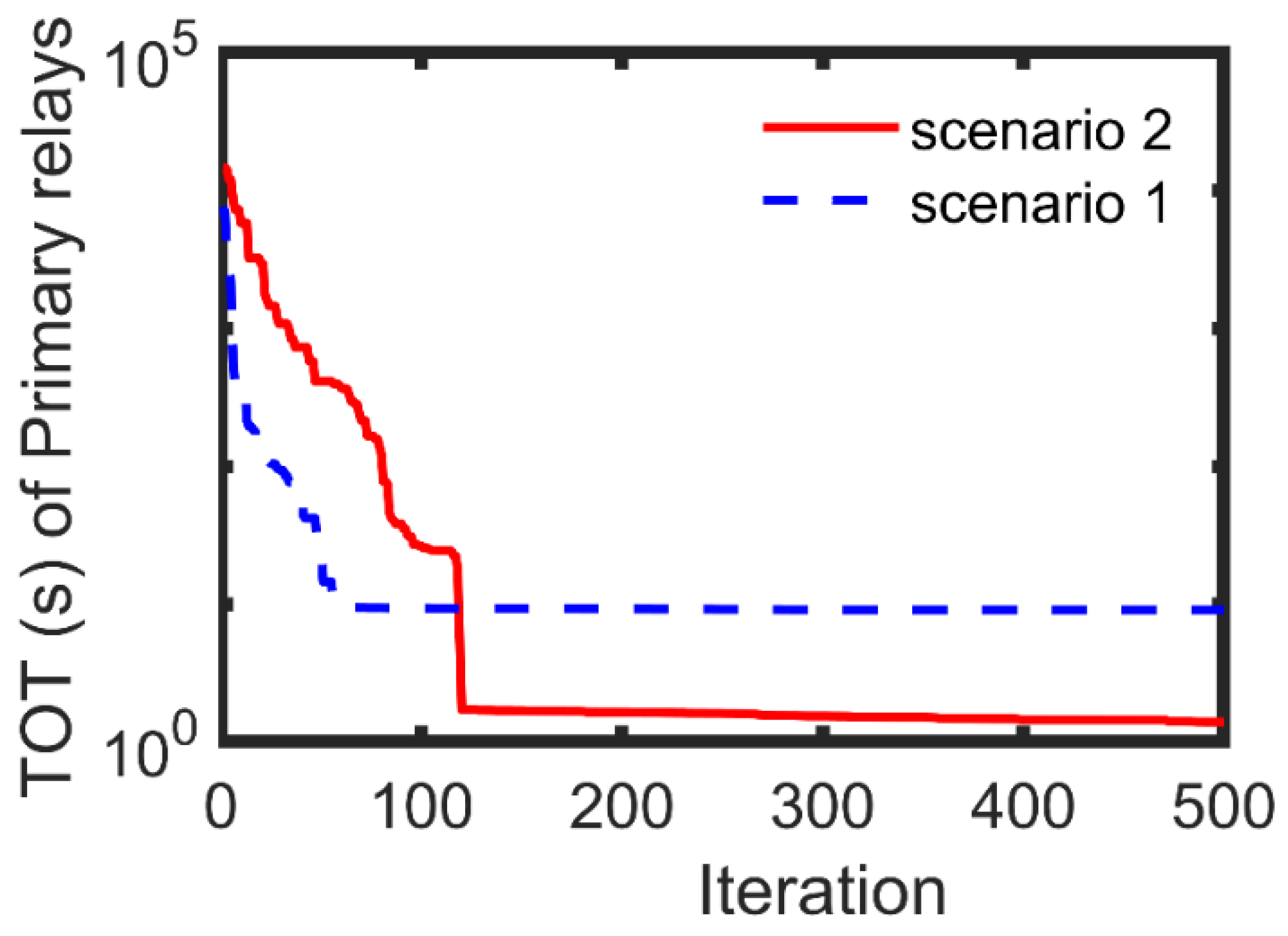
- Extracting the optimal values of the decision variables in addition to plotting the convergence trend of .
3. Procedures of the GTO
4. Study Cases and Results with Debates
4.1. Study Case 1: The IEEE 15-Bus Network
4.2. Study Case Ⅱ: The Agiba Power Network
- Transformer OCRs are fitted with the inrush inhibitor feature (2nd harmonic blocking) to transcend the inrush current during the energizing.
- Motors are started using Variable Frequency Drives (VFDs) which limit the starting current to one per unit.
- Equipment damage curves are not included in the study and considered as future works.
- Only phase OC protection coordination considering the transformers connection is performed.
- Bus coupler one and two are assumed to be closed.
- The maximum fault current condition is examined when the three DGs are in service.
- The minimum fault current condition is examined when only DG1 and DG2 are in service.
- Test Model One: Maximum three-phase fault current condition;
- Test Model Two: Maximum general fault current condition;
- Test Model Three: Minimum two-phase fault current condition; and
- Test Model Four: Minimum general fault current condition.
- The GTO succeeds in obtaining the optimal solutions without any violations in practical isolated networks with DGs using various test models.
- The OCRs’ coordination using the minimum two-phase fault current guarantees the fast convergence rate. Therefore, it is the suitable choice in online applications.
- The output p-value is minimum in test models one and two, which assures that the attained results at each run are more correlated. Accordingly, the maximum fault current coordination using the fixed NI curve is the best suitable framework in the case of a radial DG network with distribution transformers.
- The distribution of the EF currents with their optimal coordination in the case of Dy11 transformers will be a future study.
5. Conclusions
Author Contributions
Funding
Institutional Review Board Statement
Informed Consent Statement
Data Availability Statement
Conflicts of Interest
Appendix A. AGIBA Test Network Data

| ID | ||||||
|---|---|---|---|---|---|---|
| DG1 | 3250 | 11 | 20.4 | 25.3 | 189 | 80 |
| DG2 | 3250 | 11 | 20.4 | 25.3 | 189 | 80 |
| DG3 | 3250 | 11 | 20.4 | 25.3 | 189 | 80 |
| ID | Voltage Ratio (kV) | Impedance (%) | X/R | Vector Group | |
|---|---|---|---|---|---|
| TR1 | 11/3.3 | 1600 | 6.13 | 5.76 | Dy11 |
| TR2 | 11/3.3 | 1600 | 5.12 | 5.76 | Dy11 |
| TR3 | 11/3.3 | 1600 | 6.13 | 5.76 | Dy11 |
| TR4 | 11/3.3 | 1600 | 6.13 | 5.76 | Dy11 |
| TR5 | 11/3.3 | 1600 | 6.37 | 5.76 | Dy11 |
| ID | Designation | ||||
|---|---|---|---|---|---|
| MOPA | Oil Line Pump | 3.3 | 490 | 101.4 | 90.5 |
| MOPB | Oil Line Pump | 3.3 | 490 | 101.4 | 90.5 |
| MOPC | Oil Line Pump | 3.3 | 490 | 101.4 | 90.5 |
| MOPD | Oil Line Pump | 3.3 | 610 | 123.4 | 92.29 |
| WIP | Water Injection Pump | 3.3 | 607 | 125.6 | 90.5 |
| ID | Length (m) | Area (mm2) | Conductor/Insulation |
|---|---|---|---|
| F_TR1 | 10 | 25 | CU/XPLE |
| F_MCC-1 | 25 | 25 | CU/XPLE |
| F_TR2 | 10 | 25 | CU/XPLE |
| F_MCC-2 | 25 | 25 | CU/XPLE |
| F_TR3 | 10 | 25 | CU/XPLE |
| F_MCC-3 | 25 | 25 | CU/XPLE |
| F_TR4 | 10 | 25 | CU/XPLE |
| F_MCC-4 | 25 | 25 | CU/XPLE |
| F_TR5 | 10 | 25 | CU/XPLE |
| F_MOPA | 15 | 35 | CU/XPLE |
| F_MOPB | 15 | 35 | CU/XPLE |
| F_MOPC | 15 | 35 | CU/XPLE |
| F_MOPD | 15 | 35 | CU/XPLE |
| F_WIP | 15 | 35 | CU/XPLE |
| ID | ||||
|---|---|---|---|---|
| MCC-1 | 11 | 177.8 | 77.2 | 91.73 |
| MCC-2 | 11 | 90.8 | 39.2 | 91.81 |
| MCC-3 | 11 | 355.7 | 154.6 | 91.71 |
| MCC-4 | 11 | 177.8 | 77.2 | 91.73 |
| Relay ID | CTR | |
|---|---|---|
| R1 | 170.6 | 250/5 |
| R2 | 170.6 | 250/5 |
| R3 | 170.6 | 250/5 |
| R4 | 83.98 | 100/5 |
| R5 | 101.4 | 150/5 |
| R6 | 10.17 | 25/5 |
| R7 | 83.98 | 100/5 |
| R8 | 125.6 | 150/5 |
| R9 | 5.19 | 25/5 |
| R10 | 83.98 | 100/5 |
| R11 | 101.4 | 150/5 |
| R12 | 20.36 | 50/5 |
| R13 | 83.98 | 100/5 |
| R14 | 101.4 | 150/5 |
| R15 | 10.17 | 25/5 |
| R16 | 83.98 | 100/5 |
| R17 | 123.4 | 150/5 |
| Relay Pair ID | Primary | Backup | 3-Phase | 2-Phase | ||
|---|---|---|---|---|---|---|
| 1 | R5 | R4 | 3244 | 973 | 2864 | 992 |
| 2 | R4 | R1 | 2810 | 937 | 2580 | 860 |
| 3 | R4 | R2 | 2810 | 937 | 2580 | 860 |
| 4 | R4 | R3 | 2810 | 937 | 2580 | 860 |
| 5 | R6 | R1 | 2810 | 937 | 2580 | 860 |
| 6 | R6 | R2 | 2810 | 937 | 2580 | 860 |
| 7 | R6 | R3 | 2810 | 937 | 2580 | 860 |
| 8 | R8 | R7 | 3786 | 1136 | 3350 | 1160 |
| 9 | R7 | R1 | 2810 | 937 | 2580 | 860 |
| 10 | R7 | R2 | 2810 | 937 | 2580 | 860 |
| 11 | R7 | R3 | 2810 | 937 | 2580 | 860 |
| 12 | R9 | R1 | 2810 | 937 | 2580 | 860 |
| 13 | R9 | R2 | 2810 | 937 | 2580 | 860 |
| 14 | R9 | R3 | 2810 | 937 | 2580 | 860 |
| 15 | R11 | R10 | 3244 | 973 | 2864 | 992 |
| 16 | R10 | R1 | 2810 | 937 | 2580 | 860 |
| 17 | R10 | R2 | 2810 | 937 | 2580 | 860 |
| 18 | R10 | R3 | 2810 | 937 | 2580 | 860 |
| 19 | R12 | R1 | 2810 | 937 | 2580 | 860 |
| 20 | R12 | R2 | 2810 | 937 | 2580 | 860 |
| 21 | R12 | R3 | 2810 | 937 | 2580 | 860 |
| 22 | R14 | R13 | 3244 | 973 | 2864 | 992 |
| 23 | R13 | R1 | 2810 | 937 | 2580 | 860 |
| 24 | R13 | R2 | 2810 | 937 | 2580 | 860 |
| 25 | R13 | R3 | 2810 | 937 | 2580 | 860 |
| 26 | R15 | R1 | 2810 | 937 | 2580 | 860 |
| 27 | R15 | R2 | 2810 | 937 | 2580 | 860 |
| 28 | R15 | R3 | 2810 | 937 | 2580 | 860 |
| 29 | R17 | R16 | 3167 | 950 | 2794 | 968 |
| 30 | R16 | R1 | 2810 | 937 | 2580 | 860 |
| 31 | R16 | R2 | 2810 | 937 | 2580 | 860 |
| 32 | R16 | R3 | 2810 | 937 | 2580 | 860 |
| Relay Pair | Primary | Backup | 3-Phase | 2-Phase | ||
|---|---|---|---|---|---|---|
| 1 | R5 | R4 | 2505 | 751 | 2225 | 771 |
| 2 | R4 | R1 | 1669 | 835 | 1533 | 767 |
| 3 | R4 | R2 | 1669 | 835 | 1533 | 767 |
| 4 | R6 | R1 | 1669 | 835 | 1533 | 767 |
| 5 | R6 | R2 | 1669 | 835 | 1533 | 767 |
| 6 | R8 | R7 | 2879 | 864 | 2563 | 888 |
| 7 | R7 | R1 | 1669 | 835 | 1533 | 767 |
| 8 | R7 | R2 | 1669 | 835 | 1533 | 767 |
| 9 | R9 | R1 | 1669 | 835 | 1533 | 767 |
| 10 | R9 | R2 | 1669 | 835 | 1533 | 767 |
| 11 | R11 | R10 | 2505 | 751 | 2225 | 771 |
| 12 | R10 | R1 | 1669 | 835 | 1533 | 767 |
| 13 | R10 | R2 | 1669 | 835 | 1533 | 767 |
| 14 | R12 | R1 | 1669 | 835 | 1533 | 767 |
| 15 | R12 | R2 | 1669 | 835 | 1533 | 767 |
| 16 | R14 | R13 | 2505 | 751 | 2225 | 771 |
| 17 | R13 | R1 | 1669 | 835 | 1533 | 767 |
| 18 | R13 | R2 | 1669 | 835 | 1533 | 767 |
| 19 | R15 | R1 | 1669 | 835 | 1533 | 767 |
| 20 | R15 | R2 | 1669 | 835 | 1533 | 767 |
| 21 | R17 | R16 | 2452 | 736 | 2177 | 754 |
| 22 | R16 | R1 | 1669 | 835 | 1533 | 767 |
| 23 | R16 | R2 | 1669 | 835 | 1533 | 767 |
References
- Gers, J.M.; Holmes, E.J. Protection of Electricity Distribution Networks, 3rd ed.; IET Power and Energy Series 65; IET: Edison, NJ, USA, 2011; ISBN 978-1-84919-224-8. [Google Scholar]
- Draz, A.; Elkholy, M.M.; El-Fergany, A.A. Soft computing methods for attaining the protective device coordination including renewable energies: Review and prospective. Arch. Comput. Methods Eng. 2021, 28, 4383–4404. [Google Scholar] [CrossRef]
- El-Fergany, A. Protective Devices Coordination Toolbox Enhanced by an Embedded Expert System–Medium and Low Voltage Levels. In Proceedings of the 17th International Conference on Electricity Distribution, CIRED 2003, Barcelona, Spain, 12–15 May 2003; Session 3; Paper No 73. Available online: http://www.cired.net/publications/cired2003/reports/R%203-73.pdf (accessed on 23 December 2022).
- Moravej, Z.; Jazaeri, M.; Gholamzadeh, M. Optimal coordination of distance and over-current relays in series compensated systems based on MAPSO. Energy Convers. Manag. 2011, 56, 140–151. [Google Scholar] [CrossRef]
- Noghabi, A.S.; Mashhadi, H.R.; Sadeh, J. Optimal coordination of directional overcurrent relays considering different network topologies using interval linear programming. IEEE Trans. Power Deliv. 2010, 25, 1348–1354. [Google Scholar] [CrossRef]
- Srinivas, S.T.P.; Swarup, K.S. A new iterative linear programming approach to find optimal protective relay settings. Int. Trans. Electr. Energy Syst. 2020, 31, e12639. [Google Scholar] [CrossRef]
- Chabanloo, R.M.; Mohammadzadeh, N. A fast numerical method for optimal coordination of overcurrent relays in the presence of transient fault current. IET Gener. Transm. Distrib. 2018, 12, 472–481. [Google Scholar] [CrossRef]
- Bedekar, P.P.; Bhide, S.R.; Kale, V.S. Optimum time coordination of overcurrent relays using two phase simplex method. Int. J. Electr. Comput. Eng. 2009, 3, 903–907. [Google Scholar]
- Banerjee, N.; Narayanasamy, R.D.; Swathika, O.G. Optimal coordination of overcurrent relays using two phase simplex method and particle swarm optimization algorithm. In Proceedings of the International Conference on Power and Embedded Drive Control (ICPEDC), Chennai, India, 16–18 March 2017. [Google Scholar] [CrossRef]
- Birla, D.; Maheshwari, R.P.; Gupta, H.O.; Deep, K.; Thakur, M. Application of random search technique in directional overcurrent relay coordination. Int. J. Emerg. Electr. Power Syst. 2006, 7, 1–14. [Google Scholar] [CrossRef]
- Srinivas, S.T.P.; Swarup, K.S. A new mixed integer linear programming formulation for protection relay coordination using disjunctive inequalities. IEEE Power Energy Technol. Syst. J. 2020, 6, 104–112. [Google Scholar] [CrossRef]
- Draz, A.; Elkholy, M.M.; El-Fergany, A.A. Slime mould algorithm constrained by the relay operating time for optimal coordination of directional overcurrent relays using multiple standardized operating curves. Neural Comput. Appl. 2021, 33, 11875–11887. [Google Scholar] [CrossRef]
- Korashy, A.; Kamel, S.; Youssef, A.-R.; Jurado, F. Modified water cycle algorithm for optimal direction overcurrent relays coordination. Appl. Soft Comput. 2019, 74, 10–25. [Google Scholar] [CrossRef]
- El-Fergany, A.A.; Hasanien, H.M. Water cycle algorithm for optimal overcurrent relays coordination in electric power systems. Soft Comput. 2019, 23, 12761–12778. [Google Scholar] [CrossRef]
- Khurshaid, T.; Wadood, A.; Farkoush, S.G.; Yu, J.; Kim, C.-H.; Rhee, S.-B. An improved optimal solution for the directional overcurrent relays coordination using hybridized whale optimization algorithm in complex power systems. IEEE Access 2019, 7, 90418–90435. [Google Scholar] [CrossRef]
- Wadood, A.; Khurshaid, T.; Farkoush, S.G.; Yu, J.; Kim, C.-H.; Rhee, S.-B. Nature-inspired whale optimization algorithm for optimal coordination of directional overcurrent relays in power systems. Energies 2019, 12, 2297. [Google Scholar] [CrossRef]
- Khurshaid, T.; Wadood, A.; Farkoush, S.G.; Kim, C.-H.; Yu, J.; Rhee, S.-B. Improved Firefly Algorithm for the Optimal Coordination of Directional Overcurrent Relays. IEEE Access 2019, 7, 78503–78514. [Google Scholar] [CrossRef]
- Sampaio, F.C.; Tofoli, F.L.; Melo, L.S.; Barroso, G.C.; Sampaio, R.F.; Leão, R.P.S. Adaptive fuzzy directional bat algorithm for the optimal coordination of protection systems based on directional overcurrent relays. Electr. Power Syst. Res. 2022, 211, 108619. [Google Scholar] [CrossRef]
- Ferraz, R.S.F.; Ferraz, R.S.F.; Rueda-Medina, A.C.; Batista, O.E. Genetic optimisation-based distributed energy resource allocation and recloser fuse coordination. IET Gener. Transm. Distrib. 2020, 14, 4501–4508. [Google Scholar] [CrossRef]
- Korashy, A.; Kamel, S.; Alquthami, T.; Jurado, F. Optimal coordination of standard and non-standard direction overcurrent relays using an improved moth-flame optimization. IEEE Access 2020, 8, 87378–87392. [Google Scholar] [CrossRef]
- Yu, J.; Kim, C.-H.; Rhee, S.-B. The comparison of lately proposed Harris hawks optimization and JAYA optimization in solving directional overcurrent relays coordination problem. Complexity 2020, 2020, 3807653. [Google Scholar] [CrossRef]
- Yu, J.; Kim, C.-H.; Rhee, S.-B. Oppositional Jaya algorithm with distance-adaptive coefficient in solving directional over current relays coordination problem. IEEE Access 2019, 7, 150729–150742. [Google Scholar] [CrossRef]
- Irfan, M.; Wadood, A.; Khurshaid, T.; Khan, B.M.; Kim, K.-C.; Oh, S.-R.; Rhee, S.-B. An optimized adaptive protection scheme for numerical and directional overcurrent relay coordination using Harris hawk optimization. Energies 2021, 14, 5603. [Google Scholar] [CrossRef]
- Wadood, A.; Gholami Farkoush, S.; Khurshaid, T.; Kim, C.-H.; Yu, J.; Geem, Z.W.; Rhee, S.-B. An optimized protection coordination scheme for the optimal coordination of overcurrent relays using a nature-inspired root tree algorithm. Appl. Sci. 2018, 8, 1664. [Google Scholar] [CrossRef]
- Bouchekara, H.R.E.H.; Zellagui, M.; Abido, M. Optimal coordination of directional overcurrent relays using a modified electromagnetic field optimization algorithm. Appl. Soft Comput. 2017, 54, 267–283. [Google Scholar] [CrossRef]
- Vyas, D.; Bhatt, P.; Shukla, V. Coordination of directional overcurrent relays for distribution system using particle swarm optimization. Int. J. Smart Grid Clean Energy 2020, 9, 290–297. [Google Scholar] [CrossRef]
- Ramli, S.P.; Mokhlis, H.; Wong, W.R.; Muhammad, M.A.; Mansor, N.N.; Hussain, M.H. Optimal coordination of directional overcurrent relay based on combination of improved particle swarm optimization and linear programming considering multiple characteristics curve. Turk. J. Electr. Eng. Comput. Sci. 2021, 29, 1765–1780. [Google Scholar] [CrossRef]
- Khurshaid, T.; Wadood, A.; Farkoush, S.G.; Kim, C.-H.; Cho, N.; Rhee, S.-B. Modified particle swarm optimizer as optimization of time dial settings for coordination of directional overcurrent relay. J. Electr. Eng. Technol. 2019, 14, 55–68. [Google Scholar] [CrossRef]
- Gouda, E.A.; Amer, A.; Elmitwally, A. Sustained coordination of devices in a two-layer protection scheme for DGs-integrated distribution network considering system dynamics. IEEE Access 2021, 9, 111865–111878. [Google Scholar] [CrossRef]
- Elmitwally, A.; Kandil, M.S.; Gouda, E.; Amer, A. Mitigation of DGs impact on variable-topology meshed network protection system by optimal fault current limiters considering overcurrent relay coordination. Electr. Power Syst. Res. 2020, 186, 106417. [Google Scholar] [CrossRef]
- George, S.P.; Sankar, A. Optimal settings for adaptive overcurrent relay coordination in grid-connected wind farms. Electr. Power Components Syst. 2020, 48, 1308–1326. [Google Scholar] [CrossRef]
- Rizwan, M.; Hong, L.; Waseem, M.; Ahmad, S.; Sharaf, M.; Shafiq, M. A robust adaptive overcurrent relay coordination scheme for windfarm-Integrated power systems based on forecasting the wind dynamics for smart energy systems. Appl. Sci. 2020, 10, 6318. [Google Scholar] [CrossRef]
- El-Naily, N.; Saad, S.M.; Mohamed, F.A. Novel approach for optimum coordination of overcurrent relays to enhance microgrid earth fault protection scheme. Sustain. Cities Soc. 2020, 54, 102006. [Google Scholar] [CrossRef]
- Wong, J.Y.R.; Tan, C.; Abu Bakar, A.H.; Che, H.S. Selectivity problem in adaptive overcurrent protection for microgrid with inverter-based distributed generators (IBDG): Theoretical investigation and HIL verification. IEEE Trans. Power Deliv. 2022, 37, 3313–3324. [Google Scholar] [CrossRef]
- Saldarriaga-Zuluaga, S.D.; López-Lezama, J.M.; Muñoz-Galeano, N. Optimal coordination of over-current relays in microgrids considering multiple characteristic curves. Alex. Eng. J. 2021, 60, 2093–2113. [Google Scholar] [CrossRef]
- Dehghanpour, E.; Karegar, H.K.; Kheirollahi, R.; Soleymani, T. Optimal coordination of directional overcurrent relays in microgrids by using cuckoo-linear optimization algorithm and fault current limiter. IEEE Trans. Smart Grid 2018, 9, 1365–1375. [Google Scholar] [CrossRef]
- Hatata, A.; Ebeid, A.; El-Saadawi, M. Optimal restoration of directional overcurrent protection coordination for meshed distribution system integrated with DGs based on FCLs and adaptive relays. Electr. Power Syst. Res. 2022, 205, 107738. [Google Scholar] [CrossRef]
- Fayoud, A.B.; Sharaf, H.; Ibrahim, D.K. Optimal coordination of DOCRs in interconnected networks using shifted user-defined two-level characteristics. Int. J. Electr. Power Energy Syst. 2022, 142, 108298. [Google Scholar] [CrossRef]
- El-Kordy, M.; El-Fergany, A.; Gawad, A.F.A. Various metaheuristic-based algorithms for optimal relay coordination: Review and prospective. Arch. Comput. Methods Eng. 2021, 28, 3621–3629. [Google Scholar] [CrossRef]
- Rizk-Allah, R.M.; El-Fergany, A.A. Effective coordination settings for directional overcurrent relay using hybrid Gradient-based optimizer. Appl. Soft Comput. 2021, 112, 107748. [Google Scholar] [CrossRef]
- Shih, M.Y.; Conde, A.; Ángeles-Camacho, C. Enhanced self-adaptive differential evolution multi-objective algorithm for coordination of directional overcurrent relays contemplating maximum and minimum fault points. IET Gener. Transm. Distrib. 2019, 13, 4842–4852. [Google Scholar] [CrossRef]
- Tian, M.; Gao, X.; Dai, C. Differential evolution with improved individual-based parameter setting and selection strategy. Appl. Soft Comput. 2017, 56, 286–297. [Google Scholar] [CrossRef]
- Shih, M.Y.; Enríquez, A.C.; Hsiao, T.-Y.; Treviño, L.M.T. Enhanced differential evolution algorithm for coordination of directional overcurrent relays. Electr. Power Syst. Res. 2017, 143, 365–375. [Google Scholar] [CrossRef]
- El-Fergany, A.A.; Hasanien, H.M. Optimized settings of directional overcurrent relays in meshed power networks using stochastic fractal search algorithm. Int. Trans. Electr. Energy Syst. 2017, 27, e2395. [Google Scholar] [CrossRef]
- El-Fergany, A. Optimal directional digital overcurrent relays coordination and arc-flash hazard assessments in meshed networks. Int. Trans. Electr. Energy Syst. 2016, 26, 134–154. [Google Scholar] [CrossRef]
- Pandya, K.S.; Rajput, V.N. A hybrid improved harmony search algorithm-nonlinear programming approach for optimal coordination of directional overcurrent relays including characteristic selection. Int. J. Power Energy Convers. 2018, 9, 228. [Google Scholar] [CrossRef]
- Kim, C.-H.; Khurshaid, T.; Wadood, A.; Farkoush, S.G.; Rhee, S.-B. Gray wolf optimizer for the optimal coordination of directional overcurrent relay. J. Electr. Eng. Technol. 2018, 13, 1043–1051. [Google Scholar] [CrossRef]
- Srinivas, S.T.P.; Swarup, S.K. Application of improved invasive weed optimization technique for optimally setting directional overcurrent relays in power systems. Appl. Soft Comput. 2019, 79, 1–13. [Google Scholar]
- Luo, C.; Xu, Y.; Liu, Q. Using improved pollen algorithm to optimize coordination of relay protection. In Proceedings of the 10th International Conference on Power and Energy Systems (ICPES), Chengdu, China, 25–27 December 2020. [Google Scholar] [CrossRef]
- Guvenc, U.; Bakir, H.; Duman, S. Optimal coordination of directional overcurrent relays using artificial ecosystem-based optimization. In Trends in Data Engineering Methods for Intelligent Systems; Hemanth, J., Yigit, T., Patrut, B., Angelopoulou, A., Eds.; Lecture Notes on Data Engineering and Communications Technologies; Springer: Cham, Switzerland, 2021; Volume 76. [Google Scholar] [CrossRef]
- Acharya, D.; Das, D.K. Optimal coordination of over current relay using opposition learning-based gravitational search algorithm. J. Supercomput. 2021, 77, 10721–10741. [Google Scholar] [CrossRef]
- Damchi, Y.; Dolatabadi, M. Hybrid VNS–LP algorithm for online optimal coordination of directional overcurrent relays. IET Gener. Transm. Distrib. 2020, 14, 5447–5455. [Google Scholar] [CrossRef]
- Kahraman, H.T.; Bakir, H.; Duman, S.; Katı, M.; Aras, S.; Guvenc, U. Dynamic FDB selection method and its application: Modeling and optimizing of directional overcurrent relays coordination. Appl. Intell. 2021, 52, 4873–4908. [Google Scholar] [CrossRef]
- Gabr, M.A.; El-Sehiemy, R.A.; Megahed, T.F.; Ebihara, Y.; Abdelkader, S.M. Optimal settings of multiple inverter-based distributed generation for restoring coordination of DOCRs in meshed distribution networks. Electr. Power Syst. Res. 2022, 213, 108757. [Google Scholar] [CrossRef]
- Sarwagya, K.; Nayak, P.K.; Ranjan, S. Optimal coordination of directional overcurrent relays in complex distribution networks using sine cosine algorithm. Electr. Power Syst. Res. 2020, 187, 106435. [Google Scholar] [CrossRef]
- Kamel, S.; Korashy, A.; Youssef, A.-R.; Jurado, F. Development and application of an efficient optimizer for optimal coordination of direction overcurrent relays. Neural Comput. Appl. 2020, 32, 8561–8583. [Google Scholar] [CrossRef]
- Draz, A.; Elkholy, M.M.; El-Fergany, A. Over-current relays coordination including practical constraints and DGs: Damage curves, inrush, and starting currents. Sustainability 2022, 14, 2761. [Google Scholar] [CrossRef]
- Saldarriaga-Zuluaga, S.D.; López-Lezama, J.M.; Muñoz-Galeano, N. Optimal Coordination of Over-Current Relays in Microgrids Using Unsupervised Learning Techniques. Appl. Sci. 2021, 11, 1241. [Google Scholar] [CrossRef]
- Ramadan, A.; Ebeed, M.; Kamel, S.; Agwa, A.M.; Tostado-Véliz, M. The probabilistic optimal integration of renewable distributed generators considering the time-varying load based on an artificial gorilla troops optimizer. Energies 2022, 15, 1302. [Google Scholar] [CrossRef]
- Abdollahzadeh, B.; Gharehchopogh, F.S.; Mirjalili, S. Artificial gorilla troops optimizer: A new nature-inspired metaheuristic algorithm for global optimization problems. Int. J. Intell. Syst. 2021, 36, 5887–5958. [Google Scholar] [CrossRef]
- Ginidi, A.; Ghoneim, S.M.; Elsayed, A.; El-Sehiemy, R.; Shaheen, A.; El-Fergany, A. Gorilla troops optimizer for electrically based single and double-diode models of solar photovoltaic systems. Sustainability 2021, 13, 9459. [Google Scholar] [CrossRef]
- Bui, D.M.; Le, P.D.; Nguyen, T.P.; Nguyen, H. An adaptive and scalable protection coordination system of overcurrent relays in distributed-generator-integrated distribution networks. Appl. Sci. 2021, 11, 8454. [Google Scholar] [CrossRef]
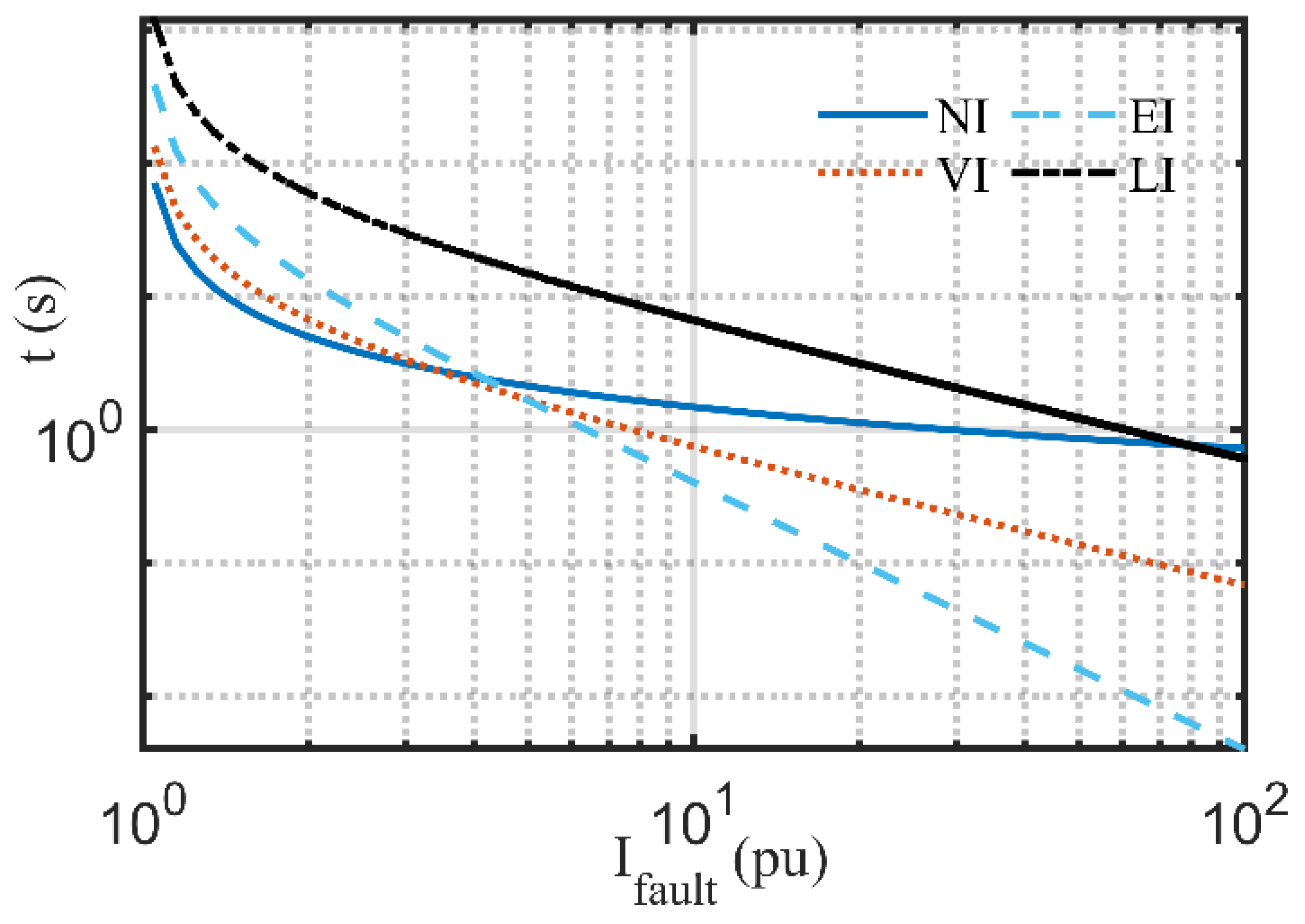


| Standard | |||
|---|---|---|---|
| IEC | NI | 0.14 | 0.02 |
| IEC | VI | 13.50 | 1.00 |
| IEC | EI | 80.00 | 2.00 |
| IEC | LI | 120.00 | 1.00 |
| Relay ID. | Scenario 1 | Scenario 2 | |||
|---|---|---|---|---|---|
| Curve | |||||
| R1 | 274.3358 | 0.0675 | 293.9991 | 0.0215 | EI |
| R2 | 313.9608 | 0.0681 | 307.6176 | 0.0244 | EI |
| R3 | 478.9256 | 0.0654 | 477.1756 | 0.0221 | EI |
| R4 | 440.9214 | 0.0663 | 442.4978 | 0.0294 | EI |
| R5 | 489.9721 | 0.0662 | 431.7093 | 0.0297 | EI |
| R6 | 373.4484 | 0.0661 | 374.9995 | 0.0264 | EI |
| R7 | 345.0252 | 0.0685 | 367.4998 | 0.0270 | EI |
| R8 | 556.5137 | 0.0668 | 559.5983 | 0.0205 | EI |
| R9 | 432.7932 | 0.0658 | 433.3580 | 0.0184 | EI |
| R10 | 403.1725 | 0.0634 | 403.8370 | 0.0199 | EI |
| R11 | 449.1812 | 0.0677 | 449.9982 | 0.0269 | EI |
| R12 | 483.8421 | 0.0666 | 502.4489 | 0.0210 | EI |
| R13 | 509.7451 | 0.0500 | 516.4943 | 0.0131 | EI |
| R14 | 394.2057 | 0.0649 | 323.7574 | 0.0338 | EI |
| R15 | 344.3698 | 0.0663 | 367.4998 | 0.0251 | EI |
| R16 | 253.7067 | 0.0639 | 245.1271 | 0.0232 | EI |
| R17 | 179.5477 | 0.0667 | 187.4989 | 0.0351 | EI |
| R18 | 457.3094 | 0.0678 | 487.9445 | 0.0204 | EI |
| R19 | 425.2535 | 0.0672 | 425.6398 | 0.0251 | EI |
| R20 | 620.0474 | 0.0641 | 622.3204 | 0.0213 | EI |
| R21 | 539.9664 | 0.0612 | 539.9992 | 0.0166 | EI |
| R22 | 202.2495 | 0.0639 | 201.8658 | 0.0244 | EI |
| R23 | 395.0120 | 0.0644 | 393.4877 | 0.0243 | EI |
| R24 | 251.1717 | 0.0653 | 224.4215 | 0.0314 | EI |
| R25 | 348.8178 | 0.0629 | 286.8513 | 0.0287 | EI |
| R26 | 304.9423 | 0.0685 | 307.2427 | 0.0383 | EI |
| R27 | 352.4827 | 0.0653 | 320.5883 | 0.0275 | EI |
| R28 | 447.8116 | 0.0667 | 389.5427 | 0.0293 | EI |
| R29 | 671.0048 | 0.0673 | 674.2527 | 0.0263 | EI |
| R30 | 201.8216 | 0.0658 | 192.8832 | 0.0310 | EI |
| R31 | 300.5795 | 0.0671 | 263.0405 | 0.0283 | EI |
| R32 | 278.9333 | 0.0661 | 284.9837 | 0.0161 | EI |
| R33 | 351.3740 | 0.0745 | 405.0106 | 0.0227 | EI |
| R34 | 298.8261 | 0.0685 | 280.2785 | 0.0308 | EI |
| R35 | 364.0380 | 0.0603 | 296.5395 | 0.0290 | EI |
| R36 | 433.7195 | 0.0676 | 382.2169 | 0.0261 | EI |
| R37 | 553.7038 | 0.0666 | 599.9994 | 0.0276 | EI |
| R38 | 299.4094 | 0.0672 | 248.6752 | 0.0331 | EI |
| R39 | 285.5946 | 0.0667 | 294.4203 | 0.0225 | EI |
| R40 | 560.6371 | 0.0670 | 490.9930 | 0.0293 | EI |
| R41 | 297.1019 | 0.0635 | 299.9973 | 0.0268 | EI |
| R42 | 337.1191 | 0.0674 | 374.1360 | 0.0164 | EI |
| TOT (s) | 9.0775 | 1.3962 | |||
| Relay Pairs | Scenario 1 | Scenario 2 | Relay Pairs | Scenario 1 | Scenario 2 | ||||||||||
|---|---|---|---|---|---|---|---|---|---|---|---|---|---|---|---|
| M | B | CTM (s) | CTM (s) | M | B | CTM (s) | CTM (s) | ||||||||
| 1 | 6 | 0.1783 | 0.3830 | 0.2047 | 0.0114 | 0.2154 | 0.2039 | 20 | 30 | 0.1742 | 0.3743 | 0.2002 | 0.0113 | 0.2162 | 0.2049 |
| 2 | 4 | 0.1730 | 0.3795 | 0.2065 | 0.0088 | 0.2320 | 0.2232 | 21 | 17 | 0.1519 | 0.3828 | 0.2309 | 0.0055 | 0.3053 | 0.2998 |
| 2 | 16 | 0.1730 | 0.4115 | 0.2385 | 0.0088 | 0.2271 | 0.2183 | 21 | 19 | 0.1519 | 0.3970 | 0.2451 | 0.0055 | 0.2135 | 0.2080 |
| 3 | 1 | 0.2115 | 0.4116 | 0.2000 | 0.0257 | 0.2319 | 0.2061 | 21 | 30 | 0.1519 | 0.3743 | 0.2224 | 0.0055 | 0.2162 | 0.2107 |
| 3 | 16 | 0.2115 | 0.4115 | 0.2000 | 0.0257 | 0.2271 | 0.2013 | 22 | 23 | 0.1930 | 0.4921 | 0.2991 | 0.0211 | 0.3744 | 0.3533 |
| 4 | 7 | 0.1976 | 0.4056 | 0.2080 | 0.0242 | 0.2655 | 0.2412 | 22 | 34 | 0.1930 | 0.4027 | 0.2097 | 0.0211 | 0.2242 | 0.2031 |
| 4 | 12 | 0.1976 | 0.4167 | 0.2191 | 0.0242 | 0.2249 | 0.2006 | 23 | 11 | 0.1744 | 0.3939 | 0.2195 | 0.0126 | 0.2212 | 0.2086 |
| 4 | 20 | 0.1976 | 0.4151 | 0.2175 | 0.0242 | 0.2287 | 0.2045 | 23 | 13 | 0.1744 | 0.4789 | 0.3046 | 0.0126 | 0.3325 | 0.3200 |
| 5 | 2 | 0.2375 | 0.4380 | 0.2005 | 0.0408 | 0.2440 | 0.2032 | 24 | 21 | 0.2021 | 0.4723 | 0.2702 | 0.0243 | 0.2634 | 0.2391 |
| 6 | 8 | 0.2318 | 0.4525 | 0.2207 | 0.0433 | 0.2467 | 0.2034 | 24 | 34 | 0.2021 | 0.4027 | 0.2006 | 0.0243 | 0.2242 | 0.2000 |
| 6 | 10 | 0.2318 | 0.4381 | 0.2063 | 0.0433 | 0.2474 | 0.2041 | 25 | 15 | 0.2295 | 0.4442 | 0.2148 | 0.0366 | 0.3377 | 0.3012 |
| 7 | 5 | 0.2377 | 0.4375 | 0.1998 | 0.0478 | 0.2506 | 0.2028 | 25 | 18 | 0.2295 | 0.4429 | 0.2134 | 0.0366 | 0.2582 | 0.2216 |
| 7 | 10 | 0.2377 | 0.4381 | 0.2004 | 0.0478 | 0.2474 | 0.1995 | 26 | 28 | 0.2325 | 0.4724 | 0.2399 | 0.0557 | 0.2799 | 0.2242 |
| 8 | 3 | 0.2147 | 0.4155 | 0.2008 | 0.0236 | 0.2237 | 0.2001 | 26 | 36 | 0.2325 | 0.4993 | 0.2668 | 0.0557 | 0.2809 | 0.2252 |
| 8 | 12 | 0.2147 | 0.4167 | 0.2020 | 0.0236 | 0.2249 | 0.2012 | 27 | 25 | 0.2580 | 0.4581 | 0.2001 | 0.0575 | 0.2573 | 0.1999 |
| 8 | 20 | 0.2147 | 0.4151 | 0.2005 | 0.0236 | 0.2287 | 0.2050 | 27 | 36 | 0.2580 | 0.4993 | 0.2413 | 0.0575 | 0.2809 | 0.2235 |
| 9 | 5 | 0.2357 | 0.4375 | 0.2018 | 0.0326 | 0.2506 | 0.2180 | 28 | 29 | 0.2654 | 0.4651 | 0.1997 | 0.0571 | 0.3316 | 0.2745 |
| 9 | 8 | 0.2357 | 0.4525 | 0.2168 | 0.0326 | 0.2467 | 0.2140 | 28 | 32 | 0.2654 | 0.5005 | 0.2352 | 0.0571 | 0.2589 | 0.2018 |
| 10 | 14 | 0.1993 | 0.4117 | 0.2124 | 0.0206 | 0.2224 | 0.2018 | 29 | 17 | 0.1821 | 0.3828 | 0.2007 | 0.0138 | 0.3053 | 0.2914 |
| 11 | 3 | 0.2042 | 0.4155 | 0.2113 | 0.0234 | 0.2237 | 0.2003 | 29 | 19 | 0.1821 | 0.3970 | 0.2149 | 0.0138 | 0.2135 | 0.1997 |
| 11 | 7 | 0.2042 | 0.4056 | 0.2014 | 0.0234 | 0.2655 | 0.2421 | 29 | 22 | 0.1821 | 0.3828 | 0.2007 | 0.0138 | 0.2139 | 0.2001 |
| 11 | 20 | 0.2042 | 0.4151 | 0.2109 | 0.0234 | 0.2287 | 0.2053 | 30 | 27 | 0.2096 | 0.4184 | 0.2089 | 0.0310 | 0.2318 | 0.2008 |
| 12 | 13 | 0.2112 | 0.4789 | 0.2677 | 0.0245 | 0.3325 | 0.3080 | 30 | 32 | 0.2096 | 0.5005 | 0.2910 | 0.0310 | 0.2589 | 0.2279 |
| 12 | 24 | 0.2112 | 0.4119 | 0.2007 | 0.0245 | 0.2452 | 0.2207 | 31 | 27 | 0.2037 | 0.4184 | 0.2147 | 0.0192 | 0.2318 | 0.2126 |
| 13 | 9 | 0.1809 | 0.5396 | 0.3587 | 0.0248 | 0.3331 | 0.3084 | 31 | 29 | 0.2037 | 0.4651 | 0.2614 | 0.0192 | 0.3316 | 0.3124 |
| 14 | 11 | 0.1804 | 0.3939 | 0.2134 | 0.0134 | 0.2212 | 0.2077 | 32 | 33 | 0.2263 | 0.4307 | 0.2044 | 0.0249 | 0.2510 | 0.2261 |
| 14 | 24 | 0.1804 | 0.4119 | 0.2315 | 0.0134 | 0.2452 | 0.2318 | 32 | 42 | 0.2263 | 0.4719 | 0.2456 | 0.0249 | 0.2697 | 0.2447 |
| 15 | 1 | 0.1729 | 0.4116 | 0.2387 | 0.0123 | 0.2319 | 0.2196 | 33 | 21 | 0.2720 | 0.4723 | 0.2003 | 0.0578 | 0.2634 | 0.2056 |
| 15 | 4 | 0.1729 | 0.3795 | 0.2065 | 0.0123 | 0.2320 | 0.2197 | 33 | 23 | 0.2720 | 0.4921 | 0.2201 | 0.0578 | 0.3744 | 0.3166 |
| 16 | 18 | 0.2014 | 0.4429 | 0.2415 | 0.0228 | 0.2582 | 0.2353 | 34 | 31 | 0.2698 | 0.4699 | 0.2001 | 0.0676 | 0.2674 | 0.1998 |
| 16 | 26 | 0.2014 | 0.4360 | 0.2345 | 0.0228 | 0.3996 | 0.3767 | 34 | 42 | 0.2698 | 0.4719 | 0.2021 | 0.0676 | 0.2697 | 0.2021 |
| 17 | 15 | 0.1944 | 0.4442 | 0.2499 | 0.0284 | 0.3377 | 0.3094 | 35 | 25 | 0.2369 | 0.4581 | 0.2212 | 0.0475 | 0.2573 | 0.2099 |
| 17 | 26 | 0.1944 | 0.4360 | 0.2416 | 0.0284 | 0.3996 | 0.3712 | 35 | 28 | 0.2369 | 0.4724 | 0.2355 | 0.0475 | 0.2799 | 0.2324 |
| 18 | 19 | 0.1581 | 0.3970 | 0.2389 | 0.0055 | 0.2135 | 0.2080 | 36 | 38 | 0.2291 | 0.4309 | 0.2018 | 0.0286 | 0.2285 | 0.1998 |
| 18 | 22 | 0.1581 | 0.3828 | 0.2247 | 0.0055 | 0.2139 | 0.2084 | 37 | 35 | 0.2564 | 0.4564 | 0.1999 | 0.0754 | 0.2759 | 0.2006 |
| 18 | 30 | 0.1581 | 0.3743 | 0.2162 | 0.0055 | 0.2162 | 0.2107 | 38 | 40 | 0.3000 | 0.5066 | 0.2066 | 0.0858 | 0.3276 | 0.2418 |
| 19 | 3 | 0.2053 | 0.4155 | 0.2102 | 0.0230 | 0.2237 | 0.2008 | 39 | 37 | 0.2847 | 0.4851 | 0.2005 | 0.0790 | 0.4681 | 0.3890 |
| 19 | 7 | 0.2053 | 0.4056 | 0.2002 | 0.0230 | 0.2655 | 0.2425 | 40 | 41 | 0.2676 | 0.4789 | 0.2113 | 0.0588 | 0.4148 | 0.3560 |
| 19 | 12 | 0.2053 | 0.4167 | 0.2114 | 0.0230 | 0.2249 | 0.2019 | 41 | 31 | 0.2304 | 0.4699 | 0.2395 | 0.0508 | 0.2674 | 0.2165 |
| 20 | 17 | 0.1742 | 0.3828 | 0.2087 | 0.0113 | 0.3053 | 0.2940 | 41 | 33 | 0.2304 | 0.4307 | 0.2003 | 0.0508 | 0.2510 | 0.2002 |
| 20 | 22 | 0.1742 | 0.3828 | 0.2087 | 0.0113 | 0.2139 | 0.2026 | 42 | 39 | 0.2022 | 0.4036 | 0.2014 | 0.0172 | 0.2174 | 0.2002 |
| Scenario 1 | Scenario 2 | |||||||
|---|---|---|---|---|---|---|---|---|
| GTO | SMA [12] | EGWO [57] | MEFO [25] | MWCA [13] | GTO | SMA [12] | SFSA [44] | FPA [45] |
| 9.0775 | 11.9761 | 12.2282 | 13.953 | 13.282 | 1.3962 | 2.4504 | 3.21 | 2.95 |
| Relay ID. | Scenario 1 | Scenario 2 | |||
|---|---|---|---|---|---|
| Curve | |||||
| R1 | 331.6117 | 0.0644 | 340.3342 | 0.0470 | VI |
| R2 | 330.5366 | 0.0604 | 341.1965 | 0.0314 | EI |
| R3 | 331.2808 | 0.0627 | 341.0609 | 0.0304 | EI |
| R4 | 167.7614 | 0.0639 | 135.9965 | 0.1137 | VI |
| R5 | 199.1274 | 0.0205 | 152.1001 | 0.2837 | EI |
| R6 | 20.3363 | 0.0370 | 15.2550 | 0.8794 | VI |
| R7 | 156.3881 | 0.0723 | 150.7917 | 0.1205 | VI |
| R8 | 226.3209 | 0.0207 | 248.9035 | 0.1443 | EI |
| R9 | 10.1672 | 0.0425 | 10.3708 | 0.9998 | VI |
| R10 | 164.7615 | 0.0646 | 167.8963 | 0.0889 | VI |
| R11 | 152.1286 | 0.0226 | 202.3552 | 0.1596 | EI |
| R12 | 40.5282 | 0.0316 | 37.4771 | 0.2736 | VI |
| R13 | 167.2944 | 0.0639 | 167.9290 | 0.1754 | EI |
| R14 | 196.5018 | 0.0206 | 202.7059 | 0.0556 | VI |
| R15 | 15.2566 | 0.0503 | 19.4621 | 0.5316 | VI |
| R16 | 163.7832 | 0.0639 | 160.8550 | 0.0909 | VI |
| R17 | 243.5889 | 0.0188 | 238.0619 | 0.1101 | EI |
| TOT (s) | 1.2509 | 0.8368 | |||
| Relay ID. | Scenario 1 | Scenario 2 | |||
|---|---|---|---|---|---|
| Curve | |||||
| R1 | 300.7964 | 0.0688 | 341.1739 | 0.0300 | EI |
| R2 | 303.7651 | 0.0674 | 341.1994 | 0.0276 | EI |
| R3 | 290.8823 | 0.0688 | 341.0980 | 0.0287 | EI |
| R4 | 154.0312 | 0.0678 | 167.8909 | 0.0909 | VI |
| R5 | 164.0629 | 0.0220 | 201.7282 | 0.1612 | EI |
| R6 | 16.5401 | 0.0387 | 20.3211 | 0.0572 | LI |
| R7 | 146.5419 | 0.0755 | 136.0492 | 0.2656 | EI |
| R8 | 251.0151 | 0.0200 | 188.4000 | 0.2519 | EI |
| R9 | 10.2956 | 0.0424 | 10.3699 | 0.9998 | VI |
| R10 | 167.5220 | 0.0647 | 166.6866 | 0.1765 | EI |
| R11 | 152.1000 | 0.0226 | 152.1013 | 0.2835 | EI |
| R12 | 40.0069 | 0.0317 | 40.6304 | 0.0284 | LI |
| R13 | 151.1998 | 0.0685 | 138.6302 | 0.1137 | VI |
| R14 | 152.1035 | 0.0226 | 167.4478 | 0.2337 | EI |
| R15 | 17.9116 | 0.0381 | 20.3392 | 0.0572 | LI |
| R16 | 125.9700 | 0.0745 | 167.6305 | 0.1751 | EI |
| R17 | 185.1458 | 0.0209 | 185.1000 | 0.1923 | EI |
| TOT (s) | 1.2614 | 0.7607 | |||
| M/B Relay Pair | Scenario 1 | Scenario 2 | |||||
|---|---|---|---|---|---|---|---|
| M | B | CTM (s) | CTM (s) | ||||
| 5 | 4 | 0.0501 | 0.2500 | 0.1999 | 0.0500 | 0.2494 | 0.1994 |
| 4 | 1 | 0.1543 | 0.4295 | 0.2753 | 0.0781 | 0.3620 | 0.2839 |
| 4 | 2 | 0.1543 | 0.4015 | 0.2472 | 0.0781 | 0.3841 | 0.3061 |
| 4 | 3 | 0.1543 | 0.4176 | 0.2634 | 0.0781 | 0.3708 | 0.2928 |
| 6 | 1 | 0.0501 | 0.4295 | 0.3794 | 0.0648 | 0.3620 | 0.2972 |
| 6 | 2 | 0.0501 | 0.4015 | 0.3514 | 0.0648 | 0.3841 | 0.3193 |
| 6 | 3 | 0.0501 | 0.4176 | 0.3676 | 0.0648 | 0.3708 | 0.3060 |
| 8 | 7 | 0.0499 | 0.2501 | 0.2002 | 0.0501 | 0.2490 | 0.1989 |
| 7 | 1 | 0.1701 | 0.4295 | 0.2594 | 0.0922 | 0.3620 | 0.2697 |
| 7 | 2 | 0.1701 | 0.4015 | 0.2313 | 0.0922 | 0.3841 | 0.2919 |
| 7 | 3 | 0.1701 | 0.4176 | 0.2475 | 0.0922 | 0.3708 | 0.2786 |
| 9 | 1 | 0.0500 | 0.4295 | 0.3795 | 0.0500 | 0.3620 | 0.3120 |
| 9 | 2 | 0.0500 | 0.4015 | 0.3515 | 0.0500 | 0.3841 | 0.3341 |
| 9 | 3 | 0.0500 | 0.4176 | 0.3677 | 0.0500 | 0.3708 | 0.3208 |
| 11 | 10 | 0.0501 | 0.2500 | 0.1999 | 0.0499 | 0.2502 | 0.2003 |
| 10 | 1 | 0.1549 | 0.4295 | 0.2746 | 0.0762 | 0.3620 | 0.2858 |
| 10 | 2 | 0.1549 | 0.4015 | 0.2466 | 0.0762 | 0.3841 | 0.3079 |
| 10 | 3 | 0.1549 | 0.4176 | 0.2628 | 0.0762 | 0.3708 | 0.2946 |
| 12 | 1 | 0.0500 | 0.4295 | 0.3795 | 0.0499 | 0.3620 | 0.3121 |
| 12 | 2 | 0.0500 | 0.4015 | 0.3515 | 0.0499 | 0.3841 | 0.3342 |
| 12 | 3 | 0.0500 | 0.4176 | 0.3676 | 0.0499 | 0.3708 | 0.3209 |
| 14 | 13 | 0.0501 | 0.2498 | 0.1997 | 0.0501 | 0.4308 | 0.3807 |
| 13 | 1 | 0.1542 | 0.4295 | 0.2753 | 0.0503 | 0.3620 | 0.3117 |
| 13 | 2 | 0.1542 | 0.4015 | 0.2473 | 0.0503 | 0.3841 | 0.3338 |
| 13 | 3 | 0.1542 | 0.4176 | 0.2634 | 0.0503 | 0.3708 | 0.3205 |
| 15 | 1 | 0.0641 | 0.4295 | 0.3654 | 0.0501 | 0.3620 | 0.3119 |
| 15 | 2 | 0.0641 | 0.4015 | 0.3374 | 0.0501 | 0.3841 | 0.3341 |
| 15 | 3 | 0.0641 | 0.4176 | 0.3536 | 0.0501 | 0.3708 | 0.3208 |
| 17 | 16 | 0.0500 | 0.2500 | 0.2000 | 0.0501 | 0.2502 | 0.2001 |
| 16 | 1 | 0.1529 | 0.4295 | 0.2766 | 0.0745 | 0.3620 | 0.2875 |
| 16 | 2 | 0.1529 | 0.4015 | 0.2486 | 0.0745 | 0.3841 | 0.3096 |
| 16 | 3 | 0.1529 | 0.4176 | 0.2647 | 0.0745 | 0.3708 | 0.2963 |
| M/B Relay Pair | Scenario 1 | Scenario 2 | |||||
|---|---|---|---|---|---|---|---|
| M | B | CTM (s) | CTM (s) | ||||
| 5 | 4 | 0.0500 | 0.2501 | 0.2000 | 0.2501 | 0.0501 | 0.2000 |
| 4 | 1 | 0.1587 | 0.4191 | 0.2603 | 0.3665 | 0.0780 | 0.2884 |
| 4 | 2 | 0.1587 | 0.4143 | 0.2556 | 0.3372 | 0.0780 | 0.2592 |
| 4 | 3 | 0.1587 | 0.4071 | 0.2484 | 0.3510 | 0.0780 | 0.2730 |
| 6 | 1 | 0.0501 | 0.4191 | 0.3690 | 0.3665 | 0.0500 | 0.3164 |
| 6 | 2 | 0.0501 | 0.4143 | 0.3642 | 0.3372 | 0.0500 | 0.2871 |
| 6 | 3 | 0.0501 | 0.4071 | 0.3570 | 0.3510 | 0.0500 | 0.3009 |
| 8 | 7 | 0.0503 | 0.2503 | 0.2000 | 0.2964 | 0.0500 | 0.2463 |
| 7 | 1 | 0.1737 | 0.4191 | 0.2453 | 0.3665 | 0.0499 | 0.3165 |
| 7 | 2 | 0.1737 | 0.4143 | 0.2406 | 0.3372 | 0.0499 | 0.2872 |
| 7 | 3 | 0.1737 | 0.4071 | 0.2333 | 0.3510 | 0.0499 | 0.3011 |
| 9 | 1 | 0.0500 | 0.4191 | 0.3691 | 0.3665 | 0.0500 | 0.3165 |
| 9 | 2 | 0.0500 | 0.4143 | 0.3643 | 0.3372 | 0.0500 | 0.2872 |
| 9 | 3 | 0.0500 | 0.4071 | 0.3571 | 0.3510 | 0.0500 | 0.3010 |
| 11 | 10 | 0.0501 | 0.2502 | 0.2001 | 0.4103 | 0.0500 | 0.3603 |
| 10 | 1 | 0.1562 | 0.4191 | 0.2629 | 0.3665 | 0.0499 | 0.3166 |
| 10 | 2 | 0.1562 | 0.4143 | 0.2582 | 0.3372 | 0.0499 | 0.2873 |
| 10 | 3 | 0.1562 | 0.4071 | 0.2509 | 0.3510 | 0.0499 | 0.3011 |
| 12 | 1 | 0.0500 | 0.4191 | 0.3691 | 0.3665 | 0.0500 | 0.3164 |
| 12 | 2 | 0.0500 | 0.4143 | 0.3643 | 0.3372 | 0.0500 | 0.2871 |
| 12 | 3 | 0.0500 | 0.4071 | 0.3571 | 0.3510 | 0.0500 | 0.3010 |
| 14 | 13 | 0.0500 | 0.2503 | 0.2003 | 0.2494 | 0.0499 | 0.1994 |
| 13 | 1 | 0.1594 | 0.4191 | 0.2596 | 0.3665 | 0.0797 | 0.2868 |
| 13 | 2 | 0.1594 | 0.4143 | 0.2549 | 0.3372 | 0.0797 | 0.2575 |
| 13 | 3 | 0.1594 | 0.4071 | 0.2476 | 0.3510 | 0.0797 | 0.2713 |
| 15 | 1 | 0.0501 | 0.4191 | 0.3690 | 0.3665 | 0.0500 | 0.3164 |
| 15 | 2 | 0.0501 | 0.4143 | 0.3643 | 0.3372 | 0.0500 | 0.2871 |
| 15 | 3 | 0.0501 | 0.4071 | 0.3570 | 0.3510 | 0.0500 | 0.3009 |
| 17 | 16 | 0.0501 | 0.2507 | 0.2005 | 0.4331 | 0.0527 | 0.3803 |
| 16 | 1 | 0.1629 | 0.4191 | 0.2562 | 0.3665 | 0.0500 | 0.3164 |
| 16 | 2 | 0.1629 | 0.4143 | 0.2515 | 0.3372 | 0.0500 | 0.2871 |
| 16 | 3 | 0.1629 | 0.4071 | 0.2442 | 0.3510 | 0.0500 | 0.3010 |
| Relay ID. | Scenario 1 | Scenario 2 | |||
|---|---|---|---|---|---|
| Curve | |||||
| R1 | 319.6939 | 0.0505 | 311.2207 | 0.0208 | EI |
| R2 | 341.1941 | 0.0491 | 340.4273 | 0.0181 | EI |
| R4 | 165.7031 | 0.0558 | 154.7975 | 0.0744 | EI |
| R5 | 200.7996 | 0.0176 | 196.5116 | 0.0795 | EI |
| R6 | 15.2550 | 0.0345 | 16.0424 | 0.0394 | LI |
| R7 | 125.9700 | 0.0712 | 131.2142 | 0.1403 | EI |
| R8 | 188.4000 | 0.0192 | 217.2035 | 0.0864 | EI |
| R9 | 7.7850 | 0.0398 | 10.3080 | 0.0616 | LI |
| R10 | 161.5779 | 0.0567 | 151.4155 | 0.0779 | EI |
| R11 | 152.1000 | 0.0197 | 183.5210 | 0.0412 | VI |
| R12 | 30.5400 | 0.0291 | 30.5400 | 0.0249 | LI |
| R13 | 125.9701 | 0.0659 | 146.6947 | 0.0832 | EI |
| R14 | 152.1000 | 0.0197 | 171.1541 | 0.1047 | EI |
| R15 | 15.2550 | 0.0345 | 20.0760 | 0.0314 | LI |
| R16 | 163.2165 | 0.0555 | 125.9700 | 0.1105 | EI |
| R17 | 201.7820 | 0.0174 | 234.5884 | 0.0532 | EI |
| TOT (s) | 1.3385 | 0.7875 | |||
| Relay ID. | Scenario 1 | Scenario 2 | |||
|---|---|---|---|---|---|
| Curve | |||||
| R1 | 300.9234 | 0.0570 | 341.1827 | 0.0197 | EI |
| R2 | 302.8060 | 0.0529 | 341.1986 | 0.0307 | VI |
| R4 | 167.5252 | 0.0544 | 125.9700 | 0.1075 | EI |
| R5 | 152.1000 | 0.0197 | 199.3379 | 0.0774 | EI |
| R6 | 15.2550 | 0.0345 | 16.4287 | 0.3422 | VI |
| R7 | 125.9701 | 0.0703 | 126.0366 | 0.1436 | EI |
| R8 | 188.4000 | 0.0193 | 188.4171 | 0.1158 | EI |
| R9 | 7.7850 | 0.0398 | 7.7872 | 0.7265 | VI |
| R10 | 125.9700 | 0.0653 | 167.3015 | 0.0599 | EI |
| R11 | 152.1003 | 0.0201 | 153.7081 | 0.0501 | VI |
| R12 | 40.6146 | 0.0269 | 40.7084 | 0.1364 | VI |
| R13 | 167.7060 | 0.0544 | 167.9591 | 0.0594 | EI |
| R14 | 202.7896 | 0.0176 | 152.1852 | 0.1332 | EI |
| R15 | 20.2051 | 0.0323 | 15.2761 | 0.3681 | VI |
| R16 | 166.9924 | 0.0538 | 165.3569 | 0.0588 | EI |
| R17 | 185.1000 | 0.0181 | 221.1283 | 0.0328 | VI |
| TOT (s) | 1.3250 | 0.7589 | |||
| M/B Relay Pair | Scenario 1 | Scenario 2 | |||||
|---|---|---|---|---|---|---|---|
| M | B | CTM (s) | CTM (s) | ||||
| 5 | 4 | 0.0499 | 0.2502 | 0.2002 | 0.0500 | 0.2499 | 0.1999 |
| 4 | 1 | 0.1717 | 0.4003 | 0.2286 | 0.0613 | 0.3273 | 0.2660 |
| 4 | 2 | 0.1717 | 0.4205 | 0.2488 | 0.0613 | 0.3554 | 0.2941 |
| 6 | 1 | 0.0500 | 0.4003 | 0.3503 | 0.0500 | 0.3273 | 0.2773 |
| 6 | 2 | 0.0500 | 0.4205 | 0.3705 | 0.0500 | 0.3554 | 0.3054 |
| 8 | 7 | 0.0502 | 0.2501 | 0.1999 | 0.0500 | 0.2505 | 0.2005 |
| 7 | 1 | 0.1944 | 0.4003 | 0.2060 | 0.0828 | 0.3273 | 0.2445 |
| 7 | 2 | 0.1944 | 0.4205 | 0.2262 | 0.0828 | 0.3554 | 0.2726 |
| 9 | 1 | 0.0500 | 0.4003 | 0.3503 | 0.0500 | 0.3273 | 0.2773 |
| 9 | 2 | 0.0500 | 0.4205 | 0.3705 | 0.0500 | 0.3554 | 0.3054 |
| 11 | 10 | 0.0500 | 0.2502 | 0.2002 | 0.0500 | 0.2499 | 0.1999 |
| 10 | 1 | 0.1726 | 0.4003 | 0.2278 | 0.0614 | 0.3273 | 0.2660 |
| 10 | 2 | 0.1726 | 0.4205 | 0.2480 | 0.0614 | 0.3554 | 0.2941 |
| 12 | 1 | 0.0500 | 0.4003 | 0.3503 | 0.0607 | 0.3273 | 0.2666 |
| 12 | 2 | 0.0500 | 0.4205 | 0.3705 | 0.0607 | 0.3554 | 0.2947 |
| 14 | 13 | 0.0500 | 0.2500 | 0.2000 | 0.0499 | 0.2500 | 0.2001 |
| 13 | 1 | 0.1800 | 0.4003 | 0.2204 | 0.0615 | 0.3273 | 0.2658 |
| 13 | 2 | 0.1800 | 0.4205 | 0.2406 | 0.0615 | 0.3554 | 0.2939 |
| 15 | 1 | 0.0501 | 0.4003 | 0.3503 | 0.0501 | 0.3273 | 0.2773 |
| 15 | 2 | 0.0501 | 0.4205 | 0.3705 | 0.0501 | 0.3554 | 0.3053 |
| 17 | 16 | 0.0499 | 0.2501 | 0.2002 | 0.0500 | 0.2538 | 0.2038 |
| 16 | 1 | 0.1697 | 0.4003 | 0.2307 | 0.0601 | 0.3273 | 0.2672 |
| 16 | 2 | 0.1697 | 0.4205 | 0.2509 | 0.0601 | 0.3554 | 0.2953 |
| M/B Relay Pair | Scenario 1 | Scenario 2 | |||||
|---|---|---|---|---|---|---|---|
| M | B | CTM (s) | CTM (s) | ||||
| 5 | 4 | 0.0501 | 0.2502 | 0.2000 | 0.0501 | 0.2490 | 0.1989 |
| 4 | 1 | 0.1683 | 0.4224 | 0.2541 | 0.0585 | 0.3892 | 0.3307 |
| 4 | 2 | 0.1683 | 0.3945 | 0.2262 | 0.0585 | 0.3321 | 0.2736 |
| 6 | 1 | 0.0499 | 0.4224 | 0.3725 | 0.0500 | 0.3892 | 0.3391 |
| 6 | 2 | 0.0499 | 0.3945 | 0.3446 | 0.0500 | 0.3321 | 0.2821 |
| 8 | 7 | 0.0505 | 0.2508 | 0.2003 | 0.0503 | 0.2498 | 0.1994 |
| 7 | 1 | 0.1922 | 0.4224 | 0.2302 | 0.0782 | 0.3892 | 0.3110 |
| 7 | 2 | 0.1922 | 0.3945 | 0.2024 | 0.0782 | 0.3321 | 0.2539 |
| 9 | 1 | 0.0500 | 0.4224 | 0.3724 | 0.0501 | 0.3892 | 0.3391 |
| 9 | 2 | 0.0500 | 0.3945 | 0.3445 | 0.0501 | 0.3321 | 0.2820 |
| 11 | 10 | 0.0511 | 0.2514 | 0.2003 | 0.0502 | 0.2502 | 0.2000 |
| 10 | 1 | 0.1783 | 0.4224 | 0.2441 | 0.0578 | 0.3892 | 0.3314 |
| 10 | 2 | 0.1783 | 0.3945 | 0.2162 | 0.0578 | 0.3321 | 0.2744 |
| 12 | 1 | 0.0501 | 0.4224 | 0.3723 | 0.0502 | 0.3892 | 0.3389 |
| 12 | 2 | 0.0501 | 0.3945 | 0.3445 | 0.0502 | 0.3321 | 0.2819 |
| 14 | 13 | 0.0504 | 0.2502 | 0.1998 | 0.0501 | 0.2503 | 0.2002 |
| 13 | 1 | 0.1683 | 0.4224 | 0.2541 | 0.0578 | 0.3892 | 0.3314 |
| 13 | 2 | 0.1683 | 0.3945 | 0.2262 | 0.0578 | 0.3321 | 0.2743 |
| 15 | 1 | 0.0501 | 0.4224 | 0.3723 | 0.0500 | 0.3892 | 0.3391 |
| 15 | 2 | 0.0501 | 0.3945 | 0.3445 | 0.0500 | 0.3321 | 0.2821 |
| 17 | 16 | 0.0500 | 0.2503 | 0.2003 | 0.0501 | 0.2500 | 0.1999 |
| 16 | 1 | 0.1662 | 0.4224 | 0.2562 | 0.0554 | 0.3892 | 0.3338 |
| 16 | 2 | 0.1662 | 0.3945 | 0.2283 | 0.0554 | 0.3321 | 0.2767 |
| Test Model | Parametric Tests | Non-Parametric Tests | Elapsed Time (s) | |||||
|---|---|---|---|---|---|---|---|---|
| Min | Max | Mean | Median | SD | p-Value | |||
| Model 1 | Scenario 1 | 1.2509 | 1.4947 | 1.3043 | 1.2839 | 0.0546 | 0 | 101.3520 |
| Scenario 2 | 0.8368 | 316.0821 | 41.4577 | 1.0940 | 91.2971 | 0.0106 | 96.4464 | |
| Model 2 | Scenario 1 | 1.2614 | 1.5560 | 1.3321 | 1.3204 | 0.0612 | 0 | 89.0859 |
| Scenario 2 | 0.7607 | 51.9367 | 4.9727 | 1.0817 | 12.1945 | 0.0343 | 99.9674 | |
| Model 3 | Scenario 1 | 1.3385 | 1.7845 | 1.4123 | 1.3814 | 0.1057 | 0.0003 | 78.1487 |
| Scenario 2 | 0.7875 | 261.3888 | 9.8377 | 1.1547 | 47.5108 | 0.1527 | 73.4870 | |
| Model 4 | Scenario 1 | 1.3250 | 1.8892 | 1.3953 | 1.3587 | 0.1082 | 0.0007 | 78.1213 |
| Scenario 2 | 0.7589 | 109.7749 | 5.5243 | 1.2019 | 20.0733 | 0.1019 | 76.3707 | |
| Test Model | Scenario | GTO | WCA |
|---|---|---|---|
| 1 | 1 | 1.2509 | 1.6962 |
| 2 | 0.8368 | 1.7862 | |
| 2 | 1 | 1.2614 | 1.6556 |
| 2 | 0.7607 | 1.4319 | |
| 3 | 1 | 1.3385 | 1.7049 |
| 2 | 0.7875 | 1.3996 | |
| 4 | 1 | 1.3250 | 1.9487 |
| 2 | 0.7589 | 1.4550 |
| M/B Relay Pair | Scenario 1 | Scenario 2 | |||||
|---|---|---|---|---|---|---|---|
| M | B | CTM (s) | CTM (s) | ||||
| 5 | 4 | 0.0552 | 0.2940 | 0.2387 | 0.0840 | 0.3394 | 0.2554 |
| 4 | 1 | 0.1903 | 0.4837 | 0.2934 | 0.1362 | 0.4365 | 0.3004 |
| 4 | 2 | 0.1903 | 0.4520 | 0.2618 | 0.1362 | 0.5035 | 0.3673 |
| 6 | 1 | 0.0562 | 0.4837 | 0.4275 | 0.1095 | 0.4365 | 0.3270 |
| 6 | 2 | 0.0562 | 0.4520 | 0.3958 | 0.1095 | 0.5035 | 0.3940 |
| 8 | 7 | 0.0555 | 0.2911 | 0.2355 | 0.0869 | 0.3439 | 0.2570 |
| 7 | 1 | 0.2087 | 0.4837 | 0.2749 | 0.1616 | 0.4365 | 0.2750 |
| 7 | 2 | 0.2087 | 0.4520 | 0.2433 | 0.1616 | 0.5035 | 0.3419 |
| 9 | 1 | 0.0554 | 0.4837 | 0.4283 | 0.0844 | 0.4365 | 0.3521 |
| 9 | 2 | 0.0554 | 0.4520 | 0.3966 | 0.0844 | 0.5035 | 0.4191 |
| 11 | 10 | 0.0549 | 0.2936 | 0.2387 | 0.0839 | 0.3456 | 0.2617 |
| 10 | 1 | 0.1908 | 0.4837 | 0.2929 | 0.1342 | 0.4365 | 0.3023 |
| 10 | 2 | 0.1908 | 0.4520 | 0.2612 | 0.1342 | 0.5035 | 0.3693 |
| 12 | 1 | 0.0573 | 0.4837 | 0.4264 | 0.0848 | 0.4365 | 0.3517 |
| 12 | 2 | 0.0573 | 0.4520 | 0.3947 | 0.0848 | 0.5035 | 0.4187 |
| 14 | 13 | 0.0552 | 0.2934 | 0.2382 | 0.0661 | 0.7385 | 0.6724 |
| 13 | 1 | 0.1900 | 0.4837 | 0.2936 | 0.1435 | 0.4365 | 0.2930 |
| 13 | 2 | 0.1900 | 0.4520 | 0.2620 | 0.1435 | 0.5035 | 0.3600 |
| 15 | 1 | 0.0715 | 0.4837 | 0.4121 | 0.0847 | 0.4365 | 0.3519 |
| 15 | 2 | 0.0715 | 0.4520 | 0.3805 | 0.0847 | 0.5035 | 0.4188 |
| 17 | 16 | 0.0557 | 0.2932 | 0.2375 | 0.0838 | 0.3432 | 0.2594 |
| 16 | 1 | 0.1882 | 0.4837 | 0.2954 | 0.1309 | 0.4365 | 0.3057 |
| 16 | 2 | 0.1882 | 0.4520 | 0.2638 | 0.1309 | 0.5035 | 0.3726 |
| M/B Relay Pair | Scenario 1 | Scenario 2 | |||||
|---|---|---|---|---|---|---|---|
| M | B | CTM (s) | CTM (s) | ||||
| 5 | 4 | 0.0575 | 0.2949 | 0.2373 | 0.1069 | 0.3533 | 0.2464 |
| 4 | 1 | 0.2018 | 0.5097 | 0.3079 | 0.1509 | 0.5920 | 0.4411 |
| 4 | 2 | 0.2018 | 0.5047 | 0.3028 | 0.1509 | 0.5447 | 0.3938 |
| 6 | 1 | 0.0571 | 0.5097 | 0.4526 | 0.0922 | 0.5920 | 0.4998 |
| 6 | 2 | 0.0571 | 0.5047 | 0.4475 | 0.0922 | 0.5447 | 0.4525 |
| 8 | 7 | 0.0589 | 0.2926 | 0.2337 | 0.1095 | 0.5402 | 0.4308 |
| 7 | 1 | 0.2199 | 0.5097 | 0.2898 | 0.1687 | 0.5920 | 0.4233 |
| 7 | 2 | 0.2199 | 0.5047 | 0.2848 | 0.1687 | 0.5447 | 0.3761 |
| 9 | 1 | 0.0564 | 0.5097 | 0.4533 | 0.0919 | 0.5920 | 0.5001 |
| 9 | 2 | 0.0564 | 0.5047 | 0.4483 | 0.0919 | 0.5447 | 0.4528 |
| 11 | 10 | 0.0574 | 0.2974 | 0.2400 | 0.1065 | 0.7316 | 0.6252 |
| 10 | 1 | 0.2001 | 0.5097 | 0.3096 | 0.1689 | 0.5920 | 0.4231 |
| 10 | 2 | 0.2001 | 0.5047 | 0.3046 | 0.1689 | 0.5447 | 0.3758 |
| 12 | 1 | 0.0587 | 0.5097 | 0.4510 | 0.0928 | 0.5920 | 0.4992 |
| 12 | 2 | 0.0587 | 0.5047 | 0.4460 | 0.0928 | 0.5447 | 0.4520 |
| 14 | 13 | 0.0574 | 0.2944 | 0.2370 | 0.1065 | 0.3475 | 0.2410 |
| 13 | 1 | 0.2022 | 0.5097 | 0.3075 | 0.1526 | 0.5920 | 0.4394 |
| 13 | 2 | 0.2022 | 0.5047 | 0.3024 | 0.1526 | 0.5447 | 0.3921 |
| 15 | 1 | 0.0573 | 0.5097 | 0.4524 | 0.0923 | 0.5920 | 0.4997 |
| 15 | 2 | 0.0573 | 0.5047 | 0.4474 | 0.0923 | 0.5447 | 0.4524 |
| 17 | 16 | 0.0579 | 0.2903 | 0.2323 | 0.1120 | 0.7664 | 0.6544 |
| 16 | 1 | 0.2035 | 0.5097 | 0.3062 | 0.1695 | 0.5920 | 0.4225 |
| 16 | 2 | 0.2035 | 0.5047 | 0.3012 | 0.1695 | 0.5447 | 0.3752 |
| M/B Relay Pair | Scenario 1 | Scenario 2 | |||||
|---|---|---|---|---|---|---|---|
| M | B | CTM (s) | CTM (s) | ||||
| 5 | 4 | 0.0451 | 0.2144 | 0.1693 | 0.0301 | 0.1486 | 0.1185 |
| 4 | 1 | 0.1334 | 0.3537 | 0.2203 | 0.0176 | 0.2508 | 0.2331 |
| 4 | 2 | 0.1334 | 0.3683 | 0.2349 | 0.0176 | 0.2691 | 0.2514 |
| 6 | 1 | 0.0438 | 0.3537 | 0.3099 | 0.0268 | 0.2508 | 0.2240 |
| 6 | 2 | 0.0438 | 0.3683 | 0.3245 | 0.0268 | 0.2691 | 0.2423 |
| 8 | 7 | 0.0454 | 0.2195 | 0.1742 | 0.0292 | 0.1455 | 0.1163 |
| 7 | 1 | 0.1549 | 0.3537 | 0.1988 | 0.0238 | 0.2508 | 0.2269 |
| 7 | 2 | 0.1549 | 0.3683 | 0.2135 | 0.0238 | 0.2691 | 0.2452 |
| 9 | 1 | 0.0445 | 0.3537 | 0.3092 | 0.0268 | 0.2508 | 0.2239 |
| 9 | 2 | 0.0445 | 0.3683 | 0.3239 | 0.0268 | 0.2691 | 0.2422 |
| 11 | 10 | 0.0456 | 0.2148 | 0.1692 | 0.0381 | 0.1487 | 0.1106 |
| 10 | 1 | 0.1344 | 0.3537 | 0.2193 | 0.0176 | 0.2508 | 0.2331 |
| 10 | 2 | 0.1344 | 0.3683 | 0.2340 | 0.0176 | 0.2691 | 0.2514 |
| 12 | 1 | 0.0429 | 0.3537 | 0.3108 | 0.0324 | 0.2508 | 0.2184 |
| 12 | 2 | 0.0429 | 0.3683 | 0.3254 | 0.0324 | 0.2691 | 0.2367 |
| 14 | 13 | 0.0456 | 0.2190 | 0.1733 | 0.0300 | 0.1488 | 0.1188 |
| 13 | 1 | 0.1433 | 0.3537 | 0.2104 | 0.0177 | 0.2508 | 0.2331 |
| 13 | 2 | 0.1433 | 0.3683 | 0.2250 | 0.0177 | 0.2691 | 0.2514 |
| 15 | 1 | 0.0438 | 0.3537 | 0.3099 | 0.0267 | 0.2508 | 0.2240 |
| 15 | 2 | 0.0438 | 0.3683 | 0.3245 | 0.0267 | 0.2691 | 0.2423 |
| 17 | 16 | 0.0451 | 0.2144 | 0.1692 | 0.0302 | 0.1523 | 0.1221 |
| 16 | 1 | 0.1320 | 0.3537 | 0.2217 | 0.0173 | 0.2508 | 0.2335 |
| 16 | 2 | 0.1320 | 0.3683 | 0.2364 | 0.0173 | 0.2691 | 0.2517 |
| M/B Relay Pair | Scenario 1 | Scenario 2 | |||||
|---|---|---|---|---|---|---|---|
| M | B | CTM (s) | CTM (s) | ||||
| 5 | 4 | 0.0437 | 0.2103 | 0.1666 | 0.0235 | 0.1410 | 0.1175 |
| 4 | 1 | 0.1313 | 0.3473 | 0.2160 | 0.0173 | 0.2409 | 0.2236 |
| 4 | 2 | 0.1313 | 0.3241 | 0.1929 | 0.0173 | 0.2373 | 0.2200 |
| 6 | 1 | 0.0439 | 0.3473 | 0.3034 | 0.0272 | 0.2409 | 0.2137 |
| 6 | 2 | 0.0439 | 0.3241 | 0.2802 | 0.0272 | 0.2373 | 0.2102 |
| 8 | 7 | 0.0437 | 0.2168 | 0.1731 | 0.0230 | 0.1372 | 0.1142 |
| 7 | 1 | 0.1536 | 0.3473 | 0.1937 | 0.0232 | 0.2409 | 0.2177 |
| 7 | 2 | 0.1536 | 0.3241 | 0.1705 | 0.0232 | 0.2373 | 0.2142 |
| 9 | 1 | 0.0446 | 0.3473 | 0.3027 | 0.0273 | 0.2409 | 0.2136 |
| 9 | 2 | 0.0446 | 0.3241 | 0.2795 | 0.0273 | 0.2373 | 0.2101 |
| 11 | 10 | 0.0446 | 0.2170 | 0.1724 | 0.0336 | 0.1403 | 0.1066 |
| 10 | 1 | 0.1427 | 0.3473 | 0.2046 | 0.0170 | 0.2409 | 0.2238 |
| 10 | 2 | 0.1427 | 0.3241 | 0.1814 | 0.0170 | 0.2373 | 0.2203 |
| 12 | 1 | 0.0426 | 0.3473 | 0.3047 | 0.0271 | 0.2409 | 0.2138 |
| 12 | 2 | 0.0426 | 0.3241 | 0.2815 | 0.0271 | 0.2373 | 0.2103 |
| 14 | 13 | 0.0432 | 0.2104 | 0.1672 | 0.0235 | 0.1402 | 0.1167 |
| 13 | 1 | 0.1313 | 0.3473 | 0.2160 | 0.0170 | 0.2409 | 0.2239 |
| 13 | 2 | 0.1313 | 0.3241 | 0.1928 | 0.0170 | 0.2373 | 0.2203 |
| 15 | 1 | 0.0436 | 0.3473 | 0.3037 | 0.0272 | 0.2409 | 0.2137 |
| 15 | 2 | 0.0436 | 0.3241 | 0.2805 | 0.0272 | 0.2373 | 0.2102 |
| 17 | 16 | 0.0434 | 0.2106 | 0.1672 | 0.0332 | 0.1414 | 0.1082 |
| 16 | 1 | 0.1297 | 0.3473 | 0.2176 | 0.0163 | 0.2409 | 0.2245 |
| 16 | 2 | 0.1297 | 0.3241 | 0.1945 | 0.0163 | 0.2373 | 0.2210 |
| Test Model No | Scenario No | Sum of CTMs | Average of CTMs | Standard Deviation |
|---|---|---|---|---|
| 1 | 1 | 7.1928 | 0.3127 | 0.0740 |
| 2 | 8.0267 | 0.3490 | 0.0882 | |
| 2 | 1 | 7.7956 | 0.3389 | 0.0868 |
| 2 | 10.0687 | 0.4378 | 0.0929 | |
| 3 | 1 | 5.6077 | 0.2438 | 0.0589 |
| 2 | 4.8509 | 0.2109 | 0.0514 | |
| 4 | 1 | 5.1629 | 0.2245 | 0.0531 |
| 2 | 4.4683 | 0.1943 | 0.0443 |
Disclaimer/Publisher’s Note: The statements, opinions and data contained in all publications are solely those of the individual author(s) and contributor(s) and not of MDPI and/or the editor(s). MDPI and/or the editor(s) disclaim responsibility for any injury to people or property resulting from any ideas, methods, instructions or products referred to in the content. |
© 2023 by the authors. Licensee MDPI, Basel, Switzerland. This article is an open access article distributed under the terms and conditions of the Creative Commons Attribution (CC BY) license (https://creativecommons.org/licenses/by/4.0/).
Share and Cite
Draz, A.; Elkholy, M.M.; El-Fergany, A.A. Automated Settings of Overcurrent Relays Considering Transformer Phase Shift and Distributed Generators Using Gorilla Troops Optimizer. Mathematics 2023, 11, 774. https://doi.org/10.3390/math11030774
Draz A, Elkholy MM, El-Fergany AA. Automated Settings of Overcurrent Relays Considering Transformer Phase Shift and Distributed Generators Using Gorilla Troops Optimizer. Mathematics. 2023; 11(3):774. https://doi.org/10.3390/math11030774
Chicago/Turabian StyleDraz, Abdelmonem, Mahmoud M. Elkholy, and Attia A. El-Fergany. 2023. "Automated Settings of Overcurrent Relays Considering Transformer Phase Shift and Distributed Generators Using Gorilla Troops Optimizer" Mathematics 11, no. 3: 774. https://doi.org/10.3390/math11030774
APA StyleDraz, A., Elkholy, M. M., & El-Fergany, A. A. (2023). Automated Settings of Overcurrent Relays Considering Transformer Phase Shift and Distributed Generators Using Gorilla Troops Optimizer. Mathematics, 11(3), 774. https://doi.org/10.3390/math11030774