A Two-State Dynamic Decomposition-Based Evolutionary Algorithm for Handling Many-Objective Optimization Problems

Abstract

Decomposition-based many-objective evolutionary algorithms (D-MaOEAs) are brilliant at keeping population diversity for predefined reference vectors or points. However, studies indicate that the performance of an D-MaOEA strongly depends on the similarity between the shape of the reference vectors (points) and that of the PF (a set of Pareto-optimal solutions symbolizing balance among objectives of many-objective optimization problems) of the many-objective problem (MaOP). Generally, MaOPs with expected PFs are not realistic. Consequently, the inevitable weak similarity results in many inactive subspaces, creating huge difficulties for maintaining diversity. To address these issues, we propose a two-state method to judge the decomposition status according to the number of inactive reference vectors. Then, two novel reference vector adjustment strategies, set as parts of the environmental selection approach, are tailored for the two states to delete inactive reference vectors and add new active reference vectors, respectively, in order to ensure that the reference vectors are as close as possible to the PF of the optimization problem. Based on the above strategies and an efficient convergence performance indicator, an active reference vector-based two-state dynamic decomposition-base MaOEA, referred to as ART-DMaOEA, is developed in this paper. Extensive experiments were conducted on ART-DMaOEA and five state-of-the-art MaOEAs on MaF1-MaF9 and WFG1-WFG9, and the comparative results show that ART-DMaOEA has the most competitive overall performance.

1. Introduction

In real-world scenarios faced by decision-makers in industrial applications, e.g., induction motor design [1], cloud computing [2,3], multiple agile earth observation satellites [4], and deep Q-learning [5], there exist many problems with two or more conflicting objectives that need to be optimized simultaneously. Such problems are referred to as multi-objective optimization problems (MOPs) by researchers. A classical MOP can be described as follows:

$$\begin{array}{cc}\min & F\left(\mathbf{x}\right)=[f_1\left(\mathbf{x}\right),f_2\left(\mathbf{x}\right),\cdots ,f_M\left(\mathbf{x}\right)],\\ \mathrm{s}.\mathrm{t}.& \mathbf{x}\in \Omega ,\end{array}$$

(1)

where $\Omega \in R$ stands for the decision space, $\mathbf{x}\in \Omega$ is a decision vector, $f_i\left(\mathbf{x}\right),i\in \{1,2,\dots ,M\}$ is the value of the ith objective, M is the number of the objective of the MOP, and $F\left(\mathbf{x}\right)$ can be considered a mapping from the decision space to the objective space. If the number of objectives of an MOP is larger than three, i.e., four or more, the MOP is usually referred to as a many-objective optimization problem (MaOP).

Due to the conflicting nature of the objectives of MOPs, progress on one objective often means deterioration of one or more other objectives, and there rarely exists one solution that can be optimal with respect to all of the objectives. Therefore, a set of Pareto-optimal solutions represents a trade-off among all the objectives pursued by the researchers. For two solutions $x_1$ and $x_2$, if $x_1$ outperforms $x_2$ on each objective, we say that $x_1$ dominates $x_2$. A solution $x\in \Omega$ can be seen as a Pareto-optimal solution if it cannot be dominated by any other solutions. For an MOP, the Pareto-optimal solutions are known as the Pareto front (PF) and the corresponding decision vectors are referred to as the Pareto set (PS). Currently, the main task of an algorithm used to solve an MOP is to obtain an approximation as close as possible to the true PF.

Multi-objective evolutionary algorithms (MOEAs) derived from traditional single-objective evolutionary algorithms (EAs) have attracted much attention for their advantageous population-based nature. In recent years, a large number of MOEAs have been developed and improved, e.g., NSGA-II [6] and MOEA/D [7]. Furthermore, as a special branch of MOPs, research into MaOPs has experience a great boom, and a variety of many-objective evolutionary algorithms (MaOEAs) have been tailored to deal with MaOPs [8,9,10].

The existing MaOEAs can be roughly divided into three categories, namely, dominance-based, decomposition-based, and indicator-based. The dominance-based MaOEAs, for instance, NSGA-III [11] and RPD-NSGA-II [12], tend to first divide solutions into different nondomination levels according to the dominance relation or other variants. Decomposition-based MaOEAs, such as RVEA [13] and MOEA/DD [14], usually transform an MaOP into several sub-MaOPs or a set of single-objective optimization problems, then solve them in a cooperative manner. In indicator-based MaOEAs, such as IGD [15] and HV [16], the performance of solutions is assigned a value based on one or more indicators.

Among the above three categories, the decomposition-based algorithms have a natural advantage in ensuring population diversity for the predefined reference vectors or points. An important branch of the decomposition-based algorithms divides an MaOP into a series of subproblems by partitioning the corresponding objective space into a set of subspaces using predefined reference vectors, for instance, MOEA/D-M2M [17] and RVEA [13]. These MaOEAs show outstanding overall performance for a variety of MaOPs, and have attracted much attention from researchers; however, a research gap in the progress of these MaOEAs remains.

As shown in Figure 1, an example is illustrated to visually show the definitions of the subspaces. In Figure 1, $S_i,i\in \{1,2,\dots ,10\}$ are ten subspaces generated by the reference vectors, while the blue points denote candidate solutions. Clearly, $S_1$ contains one solution, $S_2$ contains two solutions, $S_8$ contains two solutions, and $S_9$ contains two solutions. These subspaces are considered active subspaces, and their corresponding reference vectors are active reference vectors. By contrast, in the same example, $S_3,S_4,S_5,S_6,S_7,S_{10}$ are inactive subspaces. Obviously, the inactive subspaces fail to make a contribution to the population diversity, and can even be considered a waste of calculation resources.

In [18], Ishibuchi implies that the performance of decomposition-based MaOEAs strongly depends on the PF shapes of the candidate MaOPs. Generally, if the shape of the distribution of the weight vectors in a weight vector-based many-objective MaOEA possesses sound similarity with the shape of the PFs of the candidate MaOP, the MaOEA tends to show good performance on the MaOP. Nevertheless, predefined reference vectors cannot have high similarity with all MaOPs, as the candidate MaOPs may come from different real-world applications. When the predefined reference vectors and the PF shape of the candidate problem have a large difference, an immediate result is that more subspaces become inactive. In addition, with an increasing number of objectives of the MaOP, the objective space expands sharply, and the subspaces become large enough that even a subspace generated in the MaOP may be larger than an entire space in an MOP. Consequently, the selection of solutions in a subspace may be difficult when high diversity is expected, and reference vectors are more likely to be inactive in MaOPs. Consequently, solving MaOPs with different PFs using a decomposition-based MaOEA with a set of predefined unchanged reference vectors can encounter enormous difficulties. Figure 2 shows the variation of the proportion of the active reference vectors during the optimization process of RVEAa [19] on 10-objective MaF1. As can be seen in Figure 2, less than 45% of reference vectors are active during the process, which can be seen as a great waste of resources. Generally, more active reference vectors indicate that the region where the obtained population lies (which is a good approximation of the true PF) can be decomposed with higher adequacy. Thus, better population diversity and convergence can be expected. Under this scenario, Figure 2 obviously indicates an unexpected overall performance.

Decomposition-based MaOEAs provide a variety of suggestions and directions to solve MaOPs; however, few works have paid attention to the potential capability of active reference vectors and inactive reference vectors for maintaining diversity performance and handling MaOPs with irregular PFs. Motivated by this issue, and based on the existence of active and inactive reference vectors, a two-state scheme is proposed in this paper to divide the optimization process into two optimization states according to the proportion of the active reference vectors. These two states make for differences and similarities between the shape of the predefined reference vectors and the obtained approximation of the true PF of the candidate MaOP with different optimization methods. In order to judge which the state in which the current optimization process lies, optimization is performed in each generation on the basis of the predefined reference vectors and the obtained population. Then, two strategies are tailored for the two states of the optimization process, with the expectation that more active reference vectors are generated in the region where the PF is located. Based on the above ideas, an active reference vector-based two-state decomposition-based MaOEA is proposed to improve the population diversity and convergence of MaOPs with PFs of various shapes.

Contributions: the key contributions of this paper are listed as follows:

(1)

Two states of the optimization process are defined according to the decomposition of the obtained population, i.e., the number of the active reference vectors, to clearly identify the fit between the used MaOEA and the optimization problem.

(2)

Two strategies are tailored for the two optimization states in order to better divide the region where the true PF of the optimized MaOP is, in order to better apply population diversity pressure and avoid waste of calculation resources.

(3)

An active reference vector-based two-state decomposition-based MaOEA is proposed to improve the population diversity of MaOPs with PFs of various shapes.

The rest of this paper is organized as follows. Section 2 provides a brief review of MaOEAs. In Section 3, the specific steps of the proposed ART-DMaOEA are detailed. In Section 4, the extensive experiments and comparisons we carried out are described. In Section 5, our conclusions and possible future works are reviewed.

2. Related Studies

During the past two decades, MOEAs and MaOEAs have experienced a great boom, and a variety of algorithms have been developed and improved [20,21,22,23,24]. In MOEAs and MaOEAs, the environmental selection strategy plays a key role during the whole optimization process, and researchers tend to divide algorithms into four categories on the basis of the environmental selection strategy they use [8,25,26]: (1) dominance-based; (2) decomposition-base; (3) indicator-based; and (4) other algorithms outside of the above three categories.

This first category is mainly based on the Pareto dominance relation. These algorithms usually divide the candidate population into different dominance levels according to the inner individuals’ dominance relation, then sort the individuals in the last level using a second criterion. NSGA-II [6] is a typical dominance-based algorithm using the non-dominated sorting and crowding distance to balance convergence and diversity. In 2014, Deb et al. [11] suggested an improved version of NSGA-II called NSGA-III, in which a set of reference points are set to replace the crowding distance in NSGA-II; this approach has proven to have outstanding performance on MaOPs. SPEA2 [27] adopts a fine-grained fitness assignment strategy together with a greedy method to maintain the diversity of the obtained population. Laumanns et al. [28] developed new archiving strategies based on the concept of $\epsilon$-dominance, leading to MOEAs that have the desired convergence and distribution. Zou  et al. [29] defined a new definition of optimality (namely, L-optimality) by taking into account the number of improved objective values while considering the values of improved objective functions if all objectives have the same importance. In Ikeda et al. [30], an $\alpha$-domination strategy was proposed to relax the domination using a weak trade-off among objectives. Yuan et al. [31] defined a $\theta$-dominance relation on the basis of a reference vector-based objective space decomposition strategy and the PBI function [7]. He et al. [32] defined a fuzzy Pareto domination relation using the concept of fuzzy logic and incorporated it into NSGA-II and SPEA2 [27]. In Qiu et al. [33], considering the number of objectives on which one individual performs better than the other, the concept of fractional dominance relation was developed in order to impose sufficient selection pressure. In GrEA [34], the two concepts of grid dominance and grid difference were introduced to determine the mutual relationships of individuals in a grid environment. Tian et al. [35] proposed a new dominance relation called SDR, in which an adaptive niching technique was developed based on the angles between the candidate solutions and only the best converged candidate solution in each niche was identified as non-dominated.

Decomposition-based MOEAs and MaOEAs tend to decompose an MOP or MaOP into several subproblems and then solve them simultaneously in a collaborative manner. From the first proposal of MOEA/D by Zhang et al. [7], this branch of MOEAs has seen a rapid boom, and many variants, adaptations, and hybridizations have been developed by researchers. The approach of the existing decomposition base algorithm can be mainly divided into two categories: (1) dividing the original MOP or MaOP into several single-objective problems (SOPs), e.g., MOEA/D [7,36]; and (2) dividing the original MOP or MaOP into a group of subproblems, with the subproblems belonging to MOPs, e.g., MOEA/D-M2M [17] and RVEA [13]. Based on the above two core ideas, a number of MOEAs and MaOEAs have been developed. Wang et al. [37] defined a global replacement scheme which assigns a new solution to its most suitable subproblems. This scheme is critical for ensuring population diversity and convergence. In addition, the authors developed an approach for adjusting its size dynamically. Li et al. [38] used both differential evolution (DE) and covariance matrix adaptation in the MOEA based on decomposition, thereby clustering single-objective optimization problems into several groups. Bao et al. [39] proposed an adaptive decomposition-based evolutionary algorithm (ADEA) for both multi- and many-objective optimization. In ADEA, the candidate solutions themselves are used as RVs, meaning that the RVs can be automatically adjusted to the shape of the Pareto front (PF). In Zhao et al. [40], an adjustment was developed to update weight vectors based on the population distribution, which simulates and modifies the value function of reinforcement learning to intensify the rationality of updates. MOEA/D-M2M [17] decomposed an MOP into a set of simple MOPs through an objective space decomposition strategy. Cheng et al. [13] added a scalarization approach, termed the angle-penalized distance, to MOEA/D-M2M and proposed a reference vector adaptation strategy to dynamically adjust the distribution of the reference vectors according to the scales of the objective functions. When the second category, that is, decomposition-based MaOPs, are applied to deal with an MaOP, a variety of subspaces tend to be inactive, i.e., no individual is present in the subspace; as such, the corresponding reference vectors or points can be seen as wasteful. To mend this shortage, Cheng et al. [19] proposed an improved version of RVEA called RVEAa by randomly deleting an inactive reference vector and adding a new reference vector. The diversity-maintaining strategy of FDEA [33] can be seen as an adaptation of RVEA in which the solutions are selected using a one-by-one method instead of the one-off method used in RVEA.

Indicator-based MOEAs or MaOEAs often rank solutions using newly developed low-dimensional indicators that can represent the overall convergence and diversity performance. For instance, Zitzler et al. [41] proposed a general indicator-based evolutionary algorithm called IBEA. Emmerich et al. [42] devised a steady-state algorithm by combining the concepts of non-dominated sorting and a hypervolume-measure based selection operator, the hypervolume measure. Pamulapati et al. [43] proposed an indicator called $I_{SDE}+$, symbolizing a combination of the sum of objectives and shift-based density estimation; the ability of this indicator to promote convergence and diversity proved highly beneficial. Tian et al. [44] proposed an MOEA based on an enhanced inverted generational distance indicator, and suggested an adaptation method to adjust a set of reference points. In Dong et al. [45], a two-stage constrained multi-objective evolutionary algorithm (CMOEA) was developed with different emphases on the three indicators. Li et al. [46] proposed an enhanced indicator-based many-objective evolutionary algorithm with adaptive reference points, in which the dominance relation and the enhanced IGD-NS are used as the first selection criterion.

There are a variety of MOEAs and MaOEAs that do not fall into the above three categories. Qiu et al. [47] provided an ensemble framework for dealing with MaOPs by integrating two or more solution-sorting methods into an ensemble; in this approach, each method is considered a voter, and voters work together to decide which solutions survive to the next generation. Chen et al. [48] defined prominent solutions using the hyperplane formed by their neighboring solutions. Zhang et al. [49] tailored a decision variable clustering method to tackle large-scale MaOPs, with decision variables divided into two types, respectively, according to their relation to the convergence and diversity performance. As an alternative to ranking solutions, Yuna et al. [50] used a ratio-based indicator with an infinite norm to find promising regions in the objective space.

The ART-DMaOEA proposed in this paper belongs to the category of decomposition-based MaOEAs. In contrast with the above-mentioned strategies, our proposed algorithm first divides the optimization process into two states according to the decomposition states, then two strategies are tailored separately for the two states in order to adaptively adjust the active reference vectors. In this way, the region where the PF lies can be divided more evenly.

3. The Proposed ART-DMaOEA

3.1. The Objective Space Decomposition Strategy

MaOEAs based on an objective space decomposition strategy are an important branch of decomposition-based MaOEAs. In this paper, the objective space decomposition strategy proposed by Liu et al. [17] is adopted to divide the whole objective space into a set of subspaces using a set of predefined reference vectors.

In the objective space decomposition strategy, a set of uniformly distributed reference vectors, termed as $v_1,v_2,\cdots ,v_N$, are predefined to decompose an MOEA or MaOEA into a set of MOEAs or MaOEAs. The objective space is decomposed into N subspaces, termed as $S^1,S^2,\cdots ,S^N$, according to the acute angles between the candidate solutions and the reference vectors. Here, $S^i=\left\{p\right|\langle p,v_i\rangle \le \langle p,v_j\rangle \forall j\in 1,2,\dots ,N\}$, where $S^i$ is the ith subspace and $\langle p,v_i\rangle$ means the acute angle between p and $v_i$.

According to the definition of subspace, a solution belongs to $S^i$ if and only if the solution has the smallest angle to $v_i$ among all unit vectors. In the optimization process, each solution will be arranged into a subspace during the optimization process. In this paper, $v_i$ is the corresponding reference vector of the solutions in $S^i$.

To more vividly explain the definition of a subspace, an example is shown in Figure 3. In the example, five reference vectors (including two axes) divide the bidimensional objective space into five subspaces, and the population is partitioned into five subpopulations in five subspaces. Clearly, no solution lies in $S^1$ and $S^2$; thus, $v_1$ and $v_2$ are inactive reference vectors.

3.2. Generating Reference Vectors from a Given Population

In this paper, new reference vectors need to be constructed from the obtained population. In this section, we introduce the detailed procedure of this method.

Considering a population P with population size N, the individuals in P can be denoted as $X_1,X_2,\dots ,X_N$. Here, $f\left(x_i\right)=\{f_1\left(x_i\right),f_2\left(x_i\right),\dots ,f_M\left(x_i\right)\}$, where M is the number of the objectives. First, each $X\in P$ is normalized as

$$f^{\prime }\left(X\right)=\frac{f\left(X\right)-Z^{min}}{Z^{max}-Z^{min}}$$

(2)

where $Z^{min}=\{Z_1^{min},Z_2^{min},\dots ,Z_M^{min}\}$ and $Z^{max}=\{Z_1^{max},Z_2^{max},\dots ,Z_M^{max}\}$, while $Z_i^{min}$ and $Z_i^{max},i\in \{1,2,\dots ,M\}$ are the minimum and maximal value of the ith objective among P, respectively. The normalized $f^{\prime }\left(X\right)$ therefore ranges from 0 to 1.

Then, a reference vector $r\left(X\right)$ can be constructed from x as follows:

$$r\left(X\right)=\frac{f^{\prime }\left(X\right)}{{\sum }_{j=1}^M{f}^{\prime }{\left(X\right)}_j}$$

(3)

The newly generated reference vector points from the origin to $f^{\prime }\left(X\right)$, and intersects with the simplex ${\sum }_{i=1}^M{y}_i=1$ at $r\left(X\right)$.

3.3. The Main Framework of the ART-DMaOEA

According to the classic definition of reference vectors [11], the initial point of the reference vectors used in this paper is always the coordinate origin. To be consistent with this definition, the objective values of the individuals need to be translated as follows:

$$f^{\prime }\left(X\right)=f\left(X\right)-Z^{min}$$

(4)

where $i=1,2,\dots ,N$, $f\left(X\right)$ and $f^{\prime }\left(X\right)$ are the objective vectors before and after translation, respectively, and $Z^{min}=\{z_1^{min},z_2^{min},\dots ,z_M^{min}\}$ represents the minimal objective values calculated in the population.

The role of the translation operation is twofold: (1) to guarantee that all the translated objective values are inside the first quadrant, where the extreme point of each objective function is on the corresponding coordinate axis, thereby maximizing the coverage of the reference vectors, and (2) to set the ideal point to be the origin of the coordinate system, which simplifies the formulations presented later on.

The main framework of the proposed ART-DMaOEA is listed in Algorithm 1, from which we can see that a classic elitism strategy is adopted in ART-DMaOEA. As shown in Algorithm 1, three parameters are first initialized: (1) reference vectors V (line 1); (2) an initial population with N individuals P (line 2); (3) the number of used function evaluations $FEs$ (line 3). Then, the main loop of the proposed algorithm is presented (lines 4–14). During each iteration, the algorithm performs three main steps: (1) offspring generation (lines 5–9); (2) reference vectors processing (lines 10–14); and (3) environmental selection (line 15). In lines 5–9, an offspring population $P^{\prime }$ is generated using the simulated binary crossover and polynomial mutation. Here, Q is the combined population of P and $P^{\prime }$, used in preparation for the later selection procedure. In line 8, the parent population P is an empty set, and the individuals surviving to the next iteration in the following selection procedure are included in P. In line 10, the active reference vectors in the current generation are filtered out as $V^{\prime }$. It should be noted that V is not changed in this procedure. In lines 11–12, if the number of active reference vectors exceeds half the original V, the method for the first state of the optimization process runs to deal with the active reference vectors. In this function, individuals are selected into P and excluded from Q; therefore, P and Q are listed in the output in line 11. If half of the original reference vectors V tend to be inactive (line 13), the method prepared for the second state is applied (line 14). The methods used in the two states have the same input and output; the difference lies in the specific calculation process. In line 15, based on the newly processed $V^{\prime }$, environmental selection is performed to maintain a sound balance between convergence and diversity. The main contribution of this paper is in lines 9–14, i.e., dealing with active reference and the environmental selection method.    

Algorithm 1: Main Framework of the proposed ART-DMaOEA

In each ART-DMaOEA generation, the active reference vectors $V^{\prime }$ are selected from the original reference vectors V according to the spatial distribution relationship between Q and V. The predefined V are unchanged throughout the optimization process. In addition, apart from dealing with active reference vectors, the function Strategy for the first state() and Strategy for the second state() act as components of the environmental selection method. After the two functions are performed, solutions with good diversity performance are be absorbed into P and excluded from Q.

3.4. Strategies for the Two States

In this section, the two states during the optimization process of the proposed algorithm on MaOEA and the tailored two strategies are described in detail.

First, in Algorithm 2 all the inactive reference vectors and corresponding inactive subspaces are removed. As can be seen in Algorithm 2, $V^{\prime }$ is initialized as V in line 1; then, each individual is associated with a reference vector in V according to the definition of subspace described in Section 3.1.

In lines 3–7, reference vectors with no individual associated are deleted from $V^{\prime }$, and the corresponding subspaces are deleted from S. In line 8, the remaining reference vectors in $V^{\prime }$ and subspaces in S are renumbered as $v_1,v_2,\dots ,v_{|V^{\prime }|}$ and $S^1,S^2,\dots ,S^{|V^{\prime }|}$, respectively. Note that in Algorithm 2, no change in the original set of reference vectors V is performed.

In the proposed ART-DMaOEA, we set two optimization states: (1) over half of the original reference vectors are active and can work to maintain diversity in the generation; and (2) half of the original reference vectors are inactive. In the first state, we can roughly judge that the difference between the shape of the predefined reference vectors and the obtained population (which can be seen as an approximation of the true PF of the MaOP) is not very large; therefore, we only need a slight adjustment. The second state means that there is a huge difference between the predefined reference vectors and the true PF of the MaOP, causing a strong adjustment of the reference vectors is needed.

Algorithm 2: Delete Inactive Reference Vectors

Not each MaOP experiences both states during optimization by decomposition-based MaOEAs; whether it does is determined by the difference between the shape of the true PF of the problem and the predefined reference vectors. Certain problems may be in the first state during the whole optimization process, while others may continue to fall into the second state, and still others experience both states. The strategies developed for dealing with the two states are described in Algorithm 3 and Algorithm 4, respectively.

Algorithm 3: Strategy for the first state

As shown in Algorithm 3, P and Q serve as both input and output, which is to say that the two parameters are edited by Algorithm 3. A new solution (or solutions) is admitted into P and excluded from Q. In line 1, the subspace with the largest population size among all the active subspaces is found, and its index is referred to as k. In lines 2–3, the acute angle between each individual in $S^k$ and the corresponding reference vector is calculated. The index of the individual with the largest acute angle among $S^k$ is denoted as $j_{max}$ (line 4). In lines 5–7, $S_{j_{max}}^k$ is absorbed into P from Q and the a reference vector is constructed using $S_{j_{max}}^k$. In line 8, the newly constructed reference vector is added to the set of active reference vectors for later environmental selection.

In Algorithm 3, the individual with the best diversity performance among the subspace with the largest population size is selected into the next generation and constructed as a new reference vector. The new active reference vectors (updated in line 8) tend to be more suitable for the current population. For further explanation, an example is shown in Figure 4. In Figure 4, Figure 4a provides the distribution of the original reference vectors and the obtained population, while Figure 4b shows the deletion of inactive reference vectors. The solution pointed to by the yellow arrow in Figure 4c can be seen as $S_{j_{max}}^k$, the corresponding subspace of $v_3$ can be seen as $s^k$, and $v_{new}$ represents the newly constructed reference vectors. Obviously, the new set of active reference vectors in Figure 4c can be more evenly distributed in the region where the true PF is located, making it more efficient in maintaining diversity performance for the population.

Algorithm 4: Strategy for the second state

In the second state, over half of the original reference vectors do not work, and adding only one vector in Algorithm 3 seems to be an exhausting approach to achieve the same effect as in the first state. As a result, a tailored strategy for the second state is developed, with the main steps shown in Algorithm 4. Apart from having the same input and output, the goals to be achieved by the two algorithms are similar; that is, they each seek to construct new reference vectors while selecting individuals to survive to the next generation. Unlike from the first state, in the second state more than one reference vector is constructed.

As can be seen in Algorithm 4, subspaces with two or more individuals are entered into $V_{temp}^{\prime }$ (lines 1–4). Then, each subspace in $V_{temp}^{\prime }$ is further divided only once (lines 5–17). In line 6, the first reference vectors and corresponding subspaces are recorded as $v_{first}$ and $S^{first}$, respectively. In line 7, the acute angle between each individual in $S^{first}$ and each active reference vector in $V^{\prime }$ is calculated, and the minimal acute angles of each individual in $S^{first}$ are recorded. In line 8, the individual with the maximum minimal acute angle is selected and denoted as $P^{maxmin}$. Then, $P^{manmin}$ is absorbed into P (line 9) and excluded from Q (line 10). In lines 11–12, a new reference vector is constructed using $P^{maxmin}$ and added to $V^{\prime }$. Then, $v_{first}$ is removed from $V_{temp}$ (line 13). In lines 14–17, because the active reference vectors changes, the number of individuals in certain subspaces in $V_{temp}^{\prime }$ may be less than two; therefore, they must be removed from $V_{temp}^{\prime }$. Generally, the construction of a new reference vector means that the original subspace is divided; this distribution of active reference vectors is more suitable for the optimized MaOP. The loop (lines 5–17) terminates when all of the subspaces in $V_{temp}^{\prime }$ are divided by newly constructed reference vectors.

In Algorithm 4, there are three parameters with a high similarity: (1) the original reference vectors V; (2) the active reference vectors $V^{\prime }$; and (3) the active reference vector with two or more solutions $V_{temp}^{\prime }$. While Algorithm 4 is being run, V is an invariant and $V^{\prime }$ and $V_{temp}^{\prime }$ are variants. Here, $V^{\prime }$ is selected from V in Algorithm 2 and serves as input and output parameter of Algorithm 4, while $V_{temp}^{\prime }$ is a temporary parameter of Algorithm 2 and works for the updating of $V^{\prime }$.

The key step of the strategy for the second state is selecting candidate solutions to construct new solutions, i.e., lines 6-8 in Algorithm 4. In line 7, the minimum acute angle of a solution to the existing reference vectors indicates the degree of the difference between the solution and reference vectors. The solution with the maximal minimum acute angle has the largest difference compared with the existing reference vectors in $V^{\prime }$ and is suitable for construction as a reference vector. Because $V^{\prime }$ changes when a new reference vector is added, and the maximal minimum acute angle changes as well, The loop (lines 5–17) adopts a one-by-one method instead of a one-off method, i.e., only one reference vector is selected in each iteration of the loop. Apart from selecting the individual with the best diversity performance against the active reference vectors in $V^{\prime }$, because the newly constructed reference vectors is added to $V^{\prime }$ the method of maximum minimum acute angle ensures that at most one new reference vector is added between any two adjacent active reference vectors of $V^{\prime }$ derived from V.

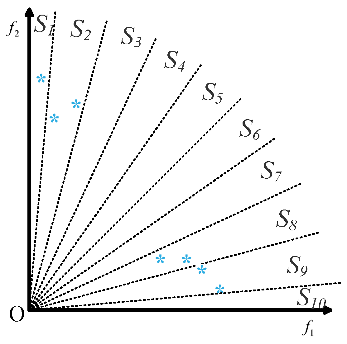
Here, we use the example shown in Figure 5 to illustrate the main steps of the strategy described in Algorithm 4. In Figure 5a, $v_0-v_9$ are ten predefined reference vectors and the red points are candidate solutions. Clearly, $v_0,v_3,v_4,v_5,v_6$ are inactive reference vectors and the other five are active reference vectors. In Figure 5b, the five inactive reference vectors are deleted and the remaining five are active reference vectors. Furthermore, the corresponding subspaces of $v_1,v_2,v_7,v_8$ each have two or more solutions. Then, following Algorithm 4, the solution in the subspace of $v_1$ is selected and constructed as a new reference vector in Figure 5b, indicated by the yellow arrow. The blue vector is the newly constructed reference vector. Figure 5c–e shows the constructed reference vectors from the corresponding subspaces of $v_2$, $v_7$, and $v_8$, respectively. Finally, the final $V^{\prime }$ output from Algorithm 4 is shown in Figure 5f.

From this example, we can easily see the core idea of the strategy developed for the second state, that is, if the predefined reference vectors are substantially different from an MaOP, the strategy can obtain a set of active reference vectors that are distributed as uniformly as possible in the region where the true PF of the optimization problem is located.

3.5. Environmental Section

The pseudocode for the environmental selection process is detailed in Algorithm 5. The purpose of the environmental selection strategy is to balance the convergence and diversity using the active reference vectors, especially the convergence performance, as the construction of the new active reference vectors in Algorithm 3 or Algorithm 4 places much attention on diversity. For this reason, the environmental selection method first selects one individual for each subspace while only considering the convergence performance, then the maximum minimum acute angle method is applied to maintain diversity for population P.

As can be seen in Algorithm 5, there are four input parameters: (1) the active reference $V^{\prime }$; (2) the individuals surviving to the next generation P; (3) the combined population Q; and (4) the population size N. Note that P is not an empty set, as Algorithm 3 or Algorithm 4 reasults in one or more individuals being absorbed into P. For each subspace (line 1), the summation of the normalized value of each solution is calculated (lines 2–3), where $S_j^i$ means the jth individuals of $S^i$ and $S_j^i\left(k\right)$ denotes the kth objective value of $S_j^i$. In lines 4–6, the individual with the least summation of normalized value in each subspace is selected into P and removed from Q.

The summation of the normalized value of an individual can reflect the convergence performance of the individual, and an individual with the least summation value always has the best convergence performance. Lines 1–6 in Algorithm 5 select the individuals with the best convergence performance into P without paying any attention to diversity. In light of this, the maximum minimum acute angle method used in the strategy developed for the second state is adopted to maintain a sound balance between convergence and diversity (lines 7–14). Because the maximum minimum acute angle method involves dynamic parameters (Q and Q), a one-by-one scheme is used instead of the one-off method. The loop continued until the size of P reaches that of N.

Algorithm 5: Environmental Selection

3.6. Time Complexity Analysis

The main time complexity of the proposed ART-DMaOEA mainly lies in lines 5–10 of Algorithms 1, 3, 4, and 5. In each generation, only one of Algorithm 3 and Algorithm 4 runs, and Algorithm 4 costs more than Algorithm 3; thus, we only need to calculate the time cost of Algorithm 4.

In Algorithm 1, line 5, it costs $O\left(DN\right)$ to generate a new population, where D denotes the number of the decision variables in an MaOP. Algorithm 1, line 9, takes $O\left(M{N}^2\right)$ to clean up the dominated solutions for all subspaces.

In Algorithm 2, it costs $O\left(M{N}^2\right)$ to associate each individual with a subspace and $O\left(N\right)$ to delete inactive reference vectors.

In Algorithm 4, it costs N to obtain $V_{temp}^{\prime }$ (lines 1–4). Then, the time complexity cost of calculating the cosines among the solutions is $O\left(M{N}^2\right)$. Next, constructing a new reference vector costs $O\left(M\right)$. As a result, the time complexity of the loop (lines 6–17) is $O\left(M{N}^3\right)$.

In Algorithm 5, it costs $O\left(M{N}^2\right)$ to calculate the summation of the objective values (lines 1–6). Then, $O\left(M{N}^3\right)$ is used to select solutions using the maximum minimum acute angle method.

To summarize, the worst-case overall computational complexity of ART-DMaOEA within one generation is $O\left(M{N}^3\right)$.

4. Experimental Studies and Discussion

To empirically investigate the overall performance of the proposed ART-DMaOEA, we compared it with the following five representative algorithm: (1) A-NSGA-III [51]; (2) BiGE [52]; (3) MOEADDU [53]; (4) RVEAa [19]; and (5) $\theta$-DEA [31].

The algorithms used in the comparative study were implemented in MATLAB 2020b, and the codes were embedded into the evolutionary multi-objective optimization platform PlatEMO [54], which is freely available on github.

4.1. Experimental Settings

4.1.1. Benchmark Test Problems

The performance of the six algorithms was compared in the context of WFG1 to WFG9 taken from WFG test suite [55] and MaF1 to MaF9 taken from MaF test suite [56], with 5, 8, 10, and 15 objectives. In this paper, a problem with a specific objective number is called a test instance, and there are 72 test instances in all from the MaF test suite and the WFG test suite. These 18 benchmarks contain various properties, e.g., disconnected, multi-modal, irregular PF, deceptiveness, etc. In this section, a benchmark with a specific number of objectives is referred to as a test instance.

4.1.2. Performance Indicators

The hypervolume (HV) [16] is used as the indicator to assess the performance of the algorithms in terms of both convergence and diversity. For an MOP or MaOP, suppose that P is the output population and $y=(y_1,y_2,\cdots ,y_M)$ is a preset reference point for the MOP. The HV value of P is the volume of the region that dominates y and is dominated by points in P. For each test instance used in this section, the reference point is set to 1.5 times the upper bound of its PF. A population with a larger HV value tends to have better overall performance. In this paper, the reference point used to calculate the HV value of a population on each test instance was embedded in PlatEMO. In addition, in this paper all of the HV values are normalized to $[0,1]$. The HV indicator has been widely used in recently research, and has been proven to have superior performance capability when dealing with MaOPs.

4.1.3. Population Size

For MOEA/D [7] and other decomposition-based algorithms, the population size is largely determined by the total number of reference points in an M-objectives problem. For problems with $M>8$, a two-layer vector generation strategy can be employed to generate reference (or weight) vectors on both the outer boundaries and the inside layers of the Pareto front [11]. Therefore, the population sizes of the six algorithms on MaF1-MaF9 are set according to the number of objectives, that is, 212, 156, 275, and 136 for 5, 8, 10, and 15 objectives, respectively.

4.1.4. Termination Conditions

The maximal number of function evaluations (MFEs) is selected as the termination condition for the six algorithms. For WFG3 and MaF3, the MFEs are set to 150,000, and for other test instances the number is 100,000. The reason for this lies in the fact that many local optimal solutions exist in WFG3 and MaF3.

4.2. Experimental Results and Analysis

To visually show the comparative results, the statistical results of the HV values of the output populations of the six algorithms on MaF1-MaF9 and WFG1-WFG9 are shown in

Table 1. HV Results of the sex algorithms on benchmarks MaF1-MaF9.

Problem	M	A-NSGA-III [51]	BiGE [52]	MOEADDU [53]	RVEAa [19]	$\mathit{\theta }$-DEA [31]	ART-DMaOEA
MaF1	5	6.9011e-3 (8.29e-4)−	1.0810e-2 (3.48e-4)−	2.6404e-3 (4.30e-4)−	7.5561e-3 (6.18e-4)−	5.5541e-3 (2.28e-4)−	1.1800e-2 (2.55e-4)
	8	2.5043e-5 (1.29e-6)+	1.8885e-5 (2.55e-6)−	1.7412e-6 (4.65e-7)−	1.0153e-5 (2.51e-6)−	2.3114e-5 (1.91e-6)+	2.3837e-5 (4.08e-6)
	10	4.6922e-7 (2.27e-8)−	2.4161e-7 (1.93e-7)−	1.3493e-8 (4.23e-9)−	7.9922e-8 (4.24e-8)−	3.3663e-7 (4.61e-8)−	6.5236e-7 (7.47e-7)
	15	2.440e-12 (4.3e-13)+	0.0000e+0 (0.00e+0)≈	1.244e-14 (4.4e-15)+	1.633e-13 (1.1e-13)+	3.691e-12 (8.35e-13)+	0.0000e+0 (0.00e+0)
MaF2	5	1.8499e-1 (2.76e-3)−	2.0191e-1 (1.62e-3)+	1.7304e-1 (1.54e-3)−	1.8888e-1 (1.91e-3)−	1.7433e-1 (4.00e-3)−	1.9250e-1 (2.02e-3)
	8	2.1073e-1 (6.11e-3)−	2.3030e-1 (2.78e-3)+	1.8416e-1 (2.30e-3)−	1.8276e-1 (4.62e-3)−	1.9479e-1 (5.86e-3)≈	2.1630e-1 (2.31e-3)
	10	2.2183e-1 (5.32e-3)+	2.3495e-1 (2.68e-3)+	1.9580e-1 (1.73e-3)−	1.7157e-1 (5.40e-3)−	1.9510e-1 (7.97e-3)−	2.1951e-1 (2.38e-3)
	15	1.6586e-1 (9.51e-3)−	2.0685e-1 (3.82e-3)+	1.3274e-1 (3.22e-3)−	1.0720e-1 (1.28e-2)−	1.6717e-1 (2.53e-3)+	1.6568e-1 (7.64e-3)
MaF3	5	9.9859e-1 (8.06e-4)−	7.5714e-1 (2.71e-1)−	9.9929e-1 (2.97e-5)+	9.9888e-1 (2.79e-4)≈	9.9338e-1 (1.21e-3)−	9.9891e-1 (1.75e-2)
	8	5.5267e-1 (4.63e-1)−	0.0000e+0 (0.00e+0)−	1.0000e+0 (1.86e-6)+	9.9981e-1 (2.06e-4)≈	9.0951e-1 (2.36e-1)−	9.926e-1 (4.58e-1)
	10	1.7003e-1 (3.66e-1)−	0.0000e+0 (0.00e+0)−	9.9821e+0 (4.49e-1)−	9.9920e-1 (3.86e-3)−	9.0484e-1 (1.54e-1)−	1.0000e-1 (0.00e+0)
	15	2.6716e-1 (4.33e-1)−	0.0000e+0 (0.00e+0)−	9.9995e-1 (2.97e-4)≈	9.9912e-1 (8.57e-4)−	8.5459e-1 (1.08e-1)−	9.9994e-1 (1.32e-4)
MaF4	5	7.2525e-2 (1.50e-2)−	1.2294e-1 (1.73e-2)+	5.0747e-4 (2.66e-3)−	1.1437e-1 (8.92e-3)+	7.6371e-2 (9.69e-3)−	9.2419e-2 (3.52e-2)
	8	1.3776e-3 (2.68e-4)−	5.0281e-3 (1.65e-4)+	0.0000e+0 (0.00e+0)−	3.9936e-4 (2.03e-4)−	2.1364e-3 (2.92e-4)+	1.5270e-3 (4.33e-4)
	10	2.4803e-5 (3.21e-5)+	4.4299e-4 (1.64e-4)+	0.0000e+0 (0.00e+0)−	9.7774e-6 (7.62e-6)−	2.1497e-4 (2.45e-5)+	1.2414e-4 (2.66e-5)
	15	2.0731e-7 (5.10e-8)+	4.1512e-7 (2.51e-8)+	0.0000e+0 (0.00e+0)≈	1.0901e-11 (1.91e-11)≈	9.9576e-8 (2.11e-8)+	0.0000e+0 (0.00e+0)
MaF5	5	7.1209e-1 (7.60e-4)−	7.9024e-1 (3.30e-3)−	7.7737e-1 (2.34e-3)−	7.7140e-1 (1.51e-2)−	8.1250e-1 (3.98e-4)+	7.9147e-1 (2.83e-3)
	8	8.2018e-1 (1.69e-3)−	9.0700e-1 (4.07e-3)≈	9.1037e-1 (5.23e-4)≈	7.9792e-1 (2.42e-2)−	9.2407e-1 (2.35e-4)+	9.0035e-1 (6.94e-3)
	10	8.6857e-1 (5.86e-4)−	7.7387e-1 (6.11e-2)−	9.5959e-1 (4.10e-4)+	8.3849e-1 (2.39e-2)−	9.7011e-1 (2.49e-4)+	9.4219e-1 (4.32e-3)
	15	9.1988e-1 (2.93e-3)−	9.7994e-1 (2.36e-3)+	9.8899e-1 (3.19e-3)+	7.6808e-1 (5.21e-2)−	9.9072e-1 (9.32e-5)+	9.2993e-1 (2.56e-2)
MaF6	5	1.2607e-1 (1.44e-3)−	1.2771e-1 (7.10e-4)−	1.1996e-1 (5.10e-4)−	1.2426e-1 (1.84e-3)−	1.1648e-1 (1.97e-3)−	1.3009e-1 (2.77e-4)
	8	6.5575e-2 (4.99e-2)−	9.3136e-2 (1.91e-2)≈	9.7182e-2 (5.43e-4)≈	1.0142e-1 (9.68e-4)+	8.5392e-2 (1.85e-2)−	8.6342e-2 (4.13e-2)
	10	3.2134e-3 (1.76e-2)≈	5.2510e-3 (1.37e-2)+	8.5614e-2 (5.18e-3)+	9.7178e-2 (3.67e-3)+	7.6600e-2 (3.90e-2)+	0.0000e+0 (0.00e+0)
	15	1.1206e-2 (1.87e-2)−	6.4103e-2 (1.53e-2)+	9.1366e-2 (3.83e-4)+	8.9473e-2 (1.70e-2)+	4.9007e-2 (3.02e-2)+	1.8864e-3 (1.03e-2)
MaF7	5	2.5548e-1 (3.74e-3)+	2.1452e-1 (4.96e-3)−	0.0000e+0 (0.00e+0)−	2.6892e-1 (3.94e-3)+	2.1857e-1 (1.03e-2)−	2.4754e-1 (3.02e-3)
	8	1.9901e-1 (2.75e-3)+	1.1274e-1 (7.39e-3)−	0.0000e+0 (0.00e+0)−	1.7061e-1 (1.57e-2)+	1.2517e-1 (5.87e-3)−	1.6421e-1 (5.57e-3)
	10	1.6567e-1 (6.36e-3)+	1.0238e-1 (9.45e-3)−	0.0000e+0 (0.00e+0)−	1.0290e-1 (2.55e-2)−	1.3093e-1 (1.16e-2)−	1.4072e-1 (5.55e-3)
	15	1.4205e-1 (1.49e-2)+	1.2131e-3 (4.40e-3)−	0.0000e+0 (0.00e+0)−	2.6686e-2 (1.88e-2)−	1.5743e-2(4.29e-3)−	8.7124e-2 (4.26e-3)
MaF8	5	1.1335e-1 (1.41e-3)−	1.1794e-1 (7.43e-4)−	8.5294e-3 (1.62e-2)−	9.9635e-2 (4.62e-3)−	8.4064e-2 (5.83e-3)−	1.2527e-1 (4.14e-4)
	8	2.5619e-2 (7.09e-4)−	2.6870e-2 (6.81e-4)−	1.3232e-2 (3.78e-3)−	1.2610e-2 (3.77e-3)−	1.6220e-2 (2.21e-3)−	3.0407e-2 (1.98e-4)
	10	9.4611e-3 (2.75e-4)−	9.6419e-3 (1.70e-4)−	1.7819e-3 (1.74e-3)−	3.5263e-3 (1.36e-3)−	5.6062e-3 (8.50e-4)−	1.0969e-2 (9.84e-5)
	15	3.6628e-4 (3.86e-5)−	4.5034e-4 (2.25e-5)−	6.3344e-5 (7.11e-5)−	8.3430e-5 (6.32e-5)−	1.6734e-4 (3.78e-5)−	5.6589e-4 (2.12e-5)
MaF9	5	1.9195e-1 (5.72e-2)−	8.8970e-2 (6.95e-2)−	2.0703e-1 (2.48e-2)+	2.6278e-1 (1.46e-2)+	1.3023e-1 (4.92e-2)−	1.9751e-1 (6.02e-2)
	8	2.0268e-2 (9.95e-3)−	4.0404e-3 (3.77e-3)−	2.1746e-2 (4.68e-3)−	1.8487e-2 (4.79e-3)−	1.9216e-2 (7.96e-3)−	3.8147e-2 (1.01e-2)
	10	9.2313e-3 (2.01e-3)−	3.9391e-4 (5.35e-4)−	3.1930e-3 (3.34e-3)−	6.0712e-3 (9.67e-4)−	6.0030e-3 (1.71e-3)−	1.6483e-2 (9.07e-4)
	15	5.3595e-4 (2.30e-4)−	4.6296e-5 (6.25e-5)−	3.4977e-4 (3.06e-4)−	2.4433e-4 (7.36e-5)−	2.3502e-4 (1.96e-4)−	7.2349e-4 (3.24e-4)
+/−/≈		8/27/1	11/22/3	11/23/2	8/25/3	12/24/1

1. +/−/≈ denotes that the corresponding result is superior to, less than, or similar to that of ART-DMaOEA. 2. The best HV results among the data proposed by the six algorithms are highlighted in gray.

and

Table 2. HV Results of the six algorithms on benchmarks WFG1-WFG9.

Problem	M	A-NSGA-III [51]	BiGE [52]	MOEADDU [53]	RVEAa [19]	$\mathit{\theta }$-DEA [31]	ART-DMaOEA
WFG1	5	9.9634e-1 (1.81e-3)−	9.9776e-1 (1.03e-3)+	9.9994e-1 (8.17e-5)+	9.3759e-1 (7.41e-2)+	9.9647e-1 (8.39e-4)≈	9.9662e-1 (6.62e-4)
	8	9.9951e-1 (2.66e-4)≈	9.9591e-1 (1.52e-3)−	9.8027e-1 (5.34e-2)−	9.5890e-1 (5.84e-2)−	9.9625e-1 (8.44e-4)−	9.9922e-1 (2.46e-4)
	10	9.9634e-1 (1.81e-3)+	9.9776e-1 (1.03e-3)+	9.9994e-1 (8.17e-5)+	9.3759e-1 (7.41e-2)−	9.9647e-1 (8.39e-4)+	9.8386e-1 (3.01e-2)
	15	9.9951e-1 (2.66e-4)−	9.9591e-1 (1.52e-3)−	9.8027e-1 (5.34e-2)−	9.5890e-1 (5.84e-2)≈	9.9625e-1 (8.44e-4)−	9.9977e-1 (1.56e-4)
WFG2	5	9.8921e-1 (2.16e-3)−	9.9479e-1 (7.43e-4)+	9.9608e-1 (1.18e-3)+	9.7968e-1 (3.32e-3)−	9.9311e-1 (8.74e-4)≈	9.9246e-1 (9.82e-4)
	8	9.9460e-1 (3.23e-3)−	9.9583e-1 (1.32e-3)≈	9.9166e-1 (4.64e-4)−	9.6189e-1 (8.04e-3)−	9.8947e-1 (3.96e-3)−	9.9530e-1 (1.05e-3)
	10	9.9554e-1 (2.33e-3)+	9.9529e-1 (1.41e-3)+	9.9896e-1 (5.52e-4)+	9.5837e-1 (7.50e-3)−	9.8716e-1 (4.16e-3)−	9.9479e-1 (1.69e-3)
	15	9.9455e-1 (2.15e-3)≈	9.9399e-1 (1.86e-3)−	9.9523e-1 (2.64e-3)≈	9.6358e-1 (1.29e-2)−	8.3090e-1 (4.77e-2)−	9.9479e-1 (2.02e-3)
WFG3	5	1.3945e-1 (1.69e-2)−	2.4533e-1 (1.59e-2)+	1.6373e-1 (1.58e-2)+	1.2037e-1 (2.19e-2)−	2.0630e-1 (9.03e-3)+	1.5095e-1 (1.56e-2)
	8	3.6749e-2 (1.70e-2)−	1.5632e-1 (1.37e-2)+	1.9183e-3 (5.74e-3)−	8.3602e-5 (4.58e-4)−	7.7782e-2 (1.31e-2)−	8.1074e-2 (5.81e-3)
	10	0.0000e+0 (0.00e+0)−	9.0492e-2 (2.53e-2)+	0.0000e+0 (0.00e+0)−	0.0000e+0 (0.00e+0)−	8.7137e-3 (1.03e-2)−	5.0858e-2 (1.56e-2)
	15	0.0000e+0 (0.00e+0)≈	0.0000e+0 (0.00e+0)≈	0.0000e+0 (0.00e+0)≈	0.0000e+0 (0.00e+0)≈	0.0000e+0 (0.00e+0)≈	0.0000e+0 (0.00e+0)
WFG4	5	7.7560e-1 (5.89e-3)+	7.9492e-1 (2.27e-3)+	7.9975e-1 (1.34e-3)+	7.6621e-1 (3.65e-3)≈	8.0052e-1 (1.30e-3)+	7.6908e-1 (3.83e-3)
	8	8.3935e-1 (1.12e-2)−	9.0980e-1 (3.54e-3)+	8.8520e-1 (7.96e-3)≈	8.2934e-1 (1.29e-2)−	9.1016e-1 (2.29e-3)+	8.8149e-1 (6.65e-3)
	10	8.8890e-1 (1.68e-2)−	8.9049e-1 (1.43e-3)−	9.4505e-1 (2.32e-3)+	8.1512e-1 (2.07e-2)−	9.3536e-1 (5.07e-3)+	9.0181e-1 (5.77e-3)
	15	9.7991e-1 (3.16e-3)+	9.7670e-1 (4.40e-3)+	7.4224e-1 (5.16e-2)−	8.5225e-1 (3.50e-2)−	9.8176e-1 (1.87e-3)+	9.1749e-1 (6.81e-3)
WFG5	5	7.4615e-1 (3.98e-3)−	7.4347e-1 (2.91e-3)−	7.4793e-1 (2.21e-3)−	7.3140e-1 (3.87e-3)≈	7.6035e-1 (4.54e-4)−	8.3208e-1 (3.93e-3)
	8	8.0775e-1 (5.98e-3)−	8.4696e-1 (3.69e-3)−	8.1864e-1 (5.00e-3)−	8.1504e-1 (4.79e-3)−	8.6049e-1 (8.57e-4)−	9.2865e-1 (4.31e-3)
	10	8.4490e-1 (5.90e-3)−	8.9697e-1 (1.44e-3)−	8.7408e-1 (2.49e-3)−	8.1846e-1 (8.57e-3)−	8.9374e-1 (1.15e-3)−	9.0720e-1 (5.93e-3)
	15	9.1485e-1 (4.56e-4)−	8.9864e-1 (8.10e-3)−	7.1548e-1 (1.76e-2)−	8.6088e-1 (1.19e-2)+	9.1448e-1 (7.42e-4)−	9.3308e-1 (5.04e-3)
WFG6	5	7.1534e-1 (1.22e-2)≈	7.2612e-1 (1.50e-2)≈	7.2503e-1 (2.10e-2)+	7.1150e-1 (1.19e-2)≈	7.0059e-1 (1.01e-2)−	7.1450e-1 (1.31e-2)
	8	7.8861e-1 (1.77e-2)−	8.3312e-1 (1.67e-2)+	7.8300e-1 (2.17e-2)−	7.5786e-1 (2.24e-2)−	8.3142e-1 (1.20e-2)+	8.2195e-1 (1.71e-2)
	10	8.2747e-1 (1.34e-2)−	8.2938e-1 (1.49e-2)−	8.4500e-1 (1.68e-2)−	7.3740e-1 (2.27e-2)−	8.2894e-1 (1.59e-2)−	8.5316e-1 (1.82e-2)
	15	8.7914e-1 (2.25e-2)+	8.9257e-1 (2.24e-2)+	7.1209e-1 (4.48e-2)−	5.9164e-1 (9.81e-2)−	8.8730e-1 (2.08e-2)+	8.5704e-1 (2.46e-2)
WFG7	5	7.8821e-1 (4.95e-3)+	7.9416e-1 (3.15e-3)≈	7.9535e-1 (7.44e-3)+	7.7656e-1 (4.36e-3)≈	8.0670e-1 (8.11e-4)−	7.8100e-1 (3.17e-3)
	8	8.5265e-1 (8.28e-3)−	9.1175e-1 (2.74e-3)≈	8.8515e-1 (1.18e-2)−	8.4496e-1 (1.16e-2)−	9.1709e-1 (9.14e-4)≈	9.1153e-1 (3.79e-3)
	10	9.0368e-1 (1.43e-2)−	9.1546e-1 (9.73e-4)−	9.4017e-1 (2.75e-3)+	8.4527e-1 (1.59e-2)−	9.5146e-1 (1.52e-3)+	9.3327e-1 (3.64e-3)
	15	9.7958e-1 (4.26e-3)+	9.2065e-1 (2.32e-3)−	8.6073e-1 (8.34e-2)−	8.4445e-1 (5.49e-2)−	9.8671e-1 (1.05e-3)+	9.4502e-1 (5.60e-3)
WFG8	5	6.2749e-1 (7.42e-3)−	6.7661e-1 (3.35e-3)−	6.6993e-1 (7.28e-3)−	6.6243e-1 (6.65e-3)−	6.8981e-1 (1.75e-3)−	9.3696e-1 (8.24e-3)
	8	7.6023e-1 (1.95e-2)−	7.9353e-1 (6.40e-3)−	7.6814e-1 (1.80e-2)−	6.8439e-1 (6.32e-2)−	7.9042e-1 (1.67e-2)−	8.0905e-1 (1.30e-2)
	10	8.3545e-1 (2.06e-2)−	8.7441e-1 (4.79e-3)−	8.7441e-1 (4.79e-3)−	7.2367e-1 (8.40e-2)−	8.4784e-1 (1.69e-2)−	8.8349e-1 (1.38e-2)
	15	8.9957e-1 (5.42e-2)−	9.1144e-1 (3.33e-3)−	6.2899e-1 (7.33e-3)−	6.5108e-1 (1.61e-1)−	9.0714e-1 (1.29e-2)−	9.3277e-1 (1.05e-2)
WFG9	5	7.3656e-1 (6.60e-3)−	7.7424e-1 (4.68e-3)−	7.5126e-1 (6.77e-3)−	7.2315e-1 (6.37e-3)≈	7.6196e-1 (3.91e-3)−	8.2986e-1 (3.38e-2)
	8	7.7633e-1 (4.30e-2)−	8.3904e-1 (8.98e-2)−	8.3136e-1 (1.17e-2)−	7.6493e-1 (2.23e-2)−	8.3342e-1 (4.29e-2)−	8.4563e-1 (7.06e-2)
	10	8.4384e-1 (3.24e-2)−	8.3319e-1 (1.84e-2)−	8.8644e-1 (8.26e-3)≈	7.5918e-1 (2.21e-2)−	8.7048e-1 (2.75e-2)−	8.9337e-1 (6.25e-2)
	15	8.5016e-1 (8.45e-2)−	8.2971e-1 (9.69e-2)−	7.0616e-1 (3.11e-2)−	7.3000e-1 (3.44e-2)−	8.6862e-1 (5.33e-2)−	8.7158e-1 (6.19e-2)
+/−/≈		7/25/4	13/20/3	10/21/5	2/27/7	10/22/4

1. +/−/≈ denotes that the corresponding result is superior to, less than, or similar to that of ART-DMaOEA. 2. The best HV results among the data proposed by the six algorithms are highlighted in gray.

, respectively. Similar to [48], the Wilcoxon rank-sum test with $\alpha =0.05$ is adopted to verify the difference between the results produced by the proposed ART-DMaOEA and those produced by the compared algorithms. In Table 1 and Table 2, the best HV results among the data proposed by the six algorithms are highlighted in gray. The symbol +/−/≈ denotes the number of test instances in which one comparative algorithm is significantly better than, worse than, or similar to the proposed ART-DMaOEA.

In

Table 3. Ratio of test cases where the corresponding baseline MaOEA performs worse than (−), better than (+), and similar to (≈) the proposed algorithm with respect to HV.

	MaF				WFG
	−	+	≈	p	−	+	≈	p
A-NSGA-III	27/36	8/36	1/36	0.0455	25/36	7/36	4/36	0.0041
BiGE	22/36	11/36	3/36	0.0128	20/36	13/36	3/36	0.0081
MOEADDU	23/36	11/36	2/36	0.063	21/36	10/36	5/36	0.013
RVEAa	25/36	8/36	2/36	0.0196	27/36	2/36	7/36	$3.2\times {10}^{-9}$
$\theta$-DEA	24/36	12/36	1/36	0.0455	22/36	10/36	4/36	0.0226

, the statistical results of the five comparative algorithms are collected. In addition, we employ the Friedman test to calculate the p values between ART-DMaOEA and each comparative algorithm in order to verify significant differences. As shown in Table 3, the p values are calculated based on the HV values of each algorithm on each test suite. From Table 3, it can be observed that most values are less than 0.05, indicating a significant difference in the results. These results demonstrate the comprehensive performance of ART-DMaOEA, as it significantly outperforms other baseline algorithms.

As can be seen in Table 1, the proposed ART-DMaOEA obtains the best result on 13 out of 36 test instances, while the numbers for the other five algorithms are 4, 7, 3, 4, and 5, respectively. Specifically, ART-DMaOEA outperforms A-NSGA-III, BiGE, MOEADDU, RVEAa, and $\theta$-DEA on 27, 22, 23, 25, and 24 out of the 36 test instances, respectively.

From Table 2, we can observe that the proposed ART-DMaOEA shows the most overall results. On 18 test instances, ART-DMaOEA shows the most competitive performance compared with the five comparative algorithms. Specifically, ART-DMaOEA outperforms A-NSGA-III, BiGE, MOEADDU, RVEAa, and $\theta$-DEA on 25, 20, 21, 27, and 22 out of the 36 test instances, respectively.

To summarize, the proposed ART-DMaOEA shows the best overall performance among the six algorithms, and shows good improvement in maintaining a balance between convergence and diversity.

To visually compare the performance of the six algorithms, their final output populations on ten-objective MaF1 and ten-objective MaF3 are plotted in parallel coordinates and illustrated in Figure 6 and Figure 7.

For ten-objective MaF1, the interval of the true PF in each objective scales from 0 to 1. From Figure 6, it can be seen that A-NSGA-III, BiGE, MOEADDU, RVEAa, and $\theta$-DEA fail to converge to the interval on certain objectives, i.e., there exist individuals with objective values larger than 1. Furthermore, the populations output by A-NSGA-III, MOEADDU, RVEAa, and $\theta$-DEA do not include individuals with objective values equal to 0. For example, the minimum value of the population output by $\theta$-DEA on all the objectives is slightly less than 0.65, rather than equal to 0. The reason for this may lie in the fact that A-NSGA-III, MOEADDU, RVEAa, and $\theta$-DEA belong to the class of decomposition-based MaOEAs, and as such their performance largely depends on the similarity of the predefined reference vectors and the true PF of the optimized MaOP. Thus, they lack enough force to adjust the reference vectors to meet the true PF of ten-objective MaF1.

MaF3 has a convex PF, and there are a large number of local fronts. This test problem is mainly used to assess whether EMaO algorithms are capable of dealing with convex PFs. As can be seen in Figure 7, it is clear that $RVEAa$ and $\theta$-DEA do not output N individuals; the reason for this is that most subspaces are inactive, causing the output population to obtain insufficient individuals. In addition, the convergence of A-NSGA-III, BiGE, and MOEADDU is very poor according to the interval of each objective of the obtained population. Specifically, the population values of A-NSGA-III in each objective dimension are distributed between $[0,7\times {10}^{10}]$ rather than 0 and 1. The same phenomena can be found in the populations of BiGE and MOEADDU. Compared with the five algorithms on ten-objective MaF1, it is apparent that the proposed algorithm has the most outstanding performance with respect to both convergence and diversity.

5. Conclusions and Future Works

This paper focuses on improving diversity performance for the existing decomposition-based MaOEAs when they are used to deal with MaOPs with PFs of various shapes. During the optimization process, we define two states according to the number of active reference vectors and inactive reference vectors. These two states indicate the similarity between the shape of the obtained population and the shape of the predefined reference vectors. High similarity means that the used MaOEA can divide the obtained population (which can be seen as a good approximation of the true PF) in an even manner, while low similarity means the opposite. Then, two strategies are tailored for the two states. The two strategies respectively aim to delete the inactive reference vectors in the generation and add new active reference vectors in order to more evenly divide the region where the obtained solutions are located. After adjustment of the active reference vectors, an efficient convergence indicator and the active reference vectors work together to strengthen convergence and diversity while maintaining a sound balance between them. To test the performance of the proposed algorithm, intensive experiments were conducted to compare it with five state-of-the-art MaOEAs on 72 test instances. The results show that the proposed ART-DMaOEA has the most competitive overall performance.

Thanks to its ability to adaptively adjust the distribution of the reference vectors according to the obtained population, ART-DMaOEA has an advantage when handling MaOPs with PFs that are unevenly distributed in the objective space. However, if it is used to solve an MaOP with a PF evenly distributed in the objective space, it may show similar performance with other MaOEAs and even sometimes be weaker. Furthermore, ART-DMaOEA has not been developed to solve MaOPs with large-scale decision variables.

Many real-world optimization problems involve various constraints and large-scale decision variables. In the future, we plan to investigate decomposition-based algorithms to solve MaOPs with large-scale decision variables or with constraints.

References

1. Salimi, A.; Lowther, D.A. Projection-based objective space reduction for many-objective optimization problems: Application to an induction motor design. In Proceedings of the 2016 IEEE Conference on Electromagnetic Field Computation (CEFC), Miami, FL, USA, 13–16 November 2016; p. 1. [Google Scholar]
2. Peng, G. Multi-objective Optimization Research and Applied in Cloud Computing. In Proceedings of the 2019 IEEE International Symposium on Software Reliability Engineering Workshops (ISSREW), Berlin, Germany, 28–31 October 2019; pp. 97–99. [Google Scholar]
3. Chen, H.; Zhu, X.; Liu, G.; Pedrycz, W. Uncertainty-aware online scheduling for real-time workflows in cloud service environment. IEEE Trans. Serv. Comput. 2021, 14, 1167–1178. [Google Scholar] [CrossRef]
4. Du, Y.; Wang, T.; Xin, B.; Wang, L.; Chen, Y.; Xing, L. A Data-Driven Parallel Scheduling Approach for Multiple Agile Earth Observation Satellites. IEEE Trans. Evol. Comput. 2020, 24, 679–693. [Google Scholar] [CrossRef]
5. Li, M.; Wang, Z.; Li, K.; Liao, X.; Hone, K.; Liu, X. Task Allocation on Layered Multiagent Systems: When Evolutionary Many-Objective Optimization Meets Deep Q-Learning. IEEE Trans. Evol. Comput. 2021, 25, 842–855. [Google Scholar] [CrossRef]
6. Deb, K.; Pratap, A.; Agarwal, S.; Meyarivan, T. A fast and elitist multiobjective genetic algorithm: NSGA-II. IEEE Trans. Evol. Comput. 2002, 6, 182–197. [Google Scholar] [CrossRef] [Green Version]
7. Zhang, Q.; Li, H. MOEA/D: A Multiobjective Evolutionary Algorithm Based on Decomposition. IEEE Trans. Evol. Comput. 2007, 11, 712–731. [Google Scholar] [CrossRef]
8. Li, B.; Li, J.; Tang, K.; Yao, X. Many-objective evolutionary algorithms: A survey. ACM Comput. Surv. (CSUR) 2015, 48, 1–35. [Google Scholar] [CrossRef] [Green Version]
9. Bechikh, S.; Elarbi, M.; Ben Said, L. Many-objective optimization using evolutionary algorithms: A survey. In Recent Advances in Evolutionary Multi-Objective Optimization; Springer: Berlin, Germany, 2017; pp. 105–137. [Google Scholar]
10. Chand, S.; Wagner, M. Evolutionary many-objective optimization: A quick-start guide. Surv. Oper. Res. Manag. Sci. 2015, 20, 35–42. [Google Scholar] [CrossRef] [Green Version]
11. Deb, K.; Jain, H. An Evolutionary Many-Objective Optimization Algorithm Using Reference-Point-Based Nondominated Sorting Approach, Part I: Solving Problems With Box Constraints. IEEE Trans. Evol. Comput. 2014, 18, 577–601. [Google Scholar] [CrossRef]
12. Elarbi, M.; Bechikh, S.; Gupta, A.; Ben Said, L.; Ong, Y.S. A New Decomposition-Based NSGA-II for Many-Objective Optimization. IEEE Trans. Syst. Man Cybern. Syst. 2018, 48, 1191–1210. [Google Scholar] [CrossRef]
13. Cheng, R.; Jin, Y.; Olhofer, M.; Sendhoff, B. A Reference Vector Guided Evolutionary Algorithm for Many-Objective Optimization. IEEE Trans. Evol. Comput. 2016, 20, 773–791. [Google Scholar] [CrossRef]
14. Li, K.; Deb, K.; Zhang, Q.; Kwong, S. An Evolutionary Many-Objective Optimization Algorithm Based on Dominance and Decomposition. IEEE Trans. Evol. Comput. 2015, 19, 694–716. [Google Scholar] [CrossRef]
15. Bosman, P.A.N.; Thierens, D. The balance between proximity and diversity in multiobjective evolutionary algorithms. IEEE Trans. Evol. Comput. 2003, 7, 174–188. [Google Scholar] [CrossRef] [Green Version]
16. Zitzler, E.; Thiele, L. Multiobjective evolutionary algorithms: A comparative case study and the strength Pareto approach. IEEE Trans. Evol. Comput. 1999, 3, 257–271. [Google Scholar] [CrossRef] [Green Version]
17. Liu, H.; Gu, F.; Zhang, Q. Decomposition of a Multiobjective Optimization Problem Into a Number of Simple Multiobjective Subproblems. IEEE Trans. Evol. Comput. 2014, 18, 450–455. [Google Scholar] [CrossRef] [Green Version]
18. Ishibuchi, H.; Setoguchi, Y.; Masuda, H.; Nojima, Y. Performance of Decomposition-Based Many-Objective Algorithms Strongly Depends on Pareto Front Shapes. IEEE Trans. Evol. Comput. 2017, 21, 169–190. [Google Scholar] [CrossRef]
19. Liu, Q.; Jin, Y.; Heiderich, M.; Rodemann, T. Adaptation of Reference Vectors for Evolutionary Many-objective Optimization of Problems with Irregular Pareto Fronts. In Proceedings of the 2019 IEEE Congress on Evolutionary Computation (CEC), Wellington, New Zealand, 10–13 June 2019; pp. 1726–1733. [Google Scholar]
20. Chen, H.; Cheng, R.; Wen, J.; Li, H.; Weng, J. Solving large-scale many-objective optimization problems by covariance matrix adaptation evolution strategy with scalable small subpopulations. Inf. Sci. 2020, 509, 457–469. [Google Scholar] [CrossRef]
21. Liu, Q.; Cui, C.; Fan, Q. Self-Adaptive Constrained Multi-Objective Differential Evolution Algorithm Based on the State–Action–Reward–State–Action Method. Mathematics 2022, 10, 813. [Google Scholar] [CrossRef]
22. Ishibuchi, H.; Tsukamoto, N.; Nojima, Y. Evolutionary many-objective optimization: A short review. In Proceedings of the 2008 IEEE Congress on Evolutionary Computation (IEEE World Congress on Computational Intelligence), Hong Kong, China, 1–6 June 2008; pp. 2419–2426. [Google Scholar]
23. Wang, Y.; Li, K.; Wang, G.G. Combining Key-Points-Based Transfer Learning and Hybrid Prediction Strategies for Dynamic Multi-Objective Optimization. Mathematics 2022, 10, 2117. [Google Scholar] [CrossRef]
24. Chen, H.; Wu, G.; Pedrycz, W.; Suganthan, P.; Xing, L.; Zhu, X. An Adaptive Resource Allocation Strategy for Objective Space Partition-Based Multiobjective Optimization. IEEE Trans. Syst. Man Cybern. Syst. 2019, 1, 1–16. [Google Scholar] [CrossRef]
25. Zhou, A.; Qu, B.Y.; Li, H.; Zhao, S.Z.; Suganthan, P.N.; Zhang, Q. Multiobjective evolutionary algorithms: A survey of the state of the art. Swarm Evol. Comput. 2011, 1, 32–49. [Google Scholar] [CrossRef]
26. Bader, J.; Zitzler, E. HypE: An Algorithm for Fast Hypervolume-Based Many-Objective Optimization. Evol. Comput. 2011, 19, 45–76. [Google Scholar] [CrossRef] [PubMed]
27. Zitzler, E.; Laumanns, M.; Thiele, L. SPEA2: Improving the Strength Pareto Evolutionary Algorithm; TIK-Report; TIK: New York, NY, USA, 2001; Volume 103. [Google Scholar]
28. Laumanns, M.; Thiele, L.; Deb, K.; Zitzler, E. Combining Convergence and Diversity in Evolutionary Multiobjective Optimization. Evol. Comput. 2002, 10, 263–282. [Google Scholar] [CrossRef] [PubMed]
29. Zou, X.; Chen, Y.; Liu, M.; Kang, L. A New Evolutionary Algorithm for Solving Many-Objective Optimization Problems. IEEE Trans. Syst. Man, Cybern. Part B Cybern. 2008, 38, 1402–1412. [Google Scholar]
30. Ikeda, K.; Kita, H.; Kobayashi, S. Failure of Pareto-based MOEAs: Does non-dominated really mean near to optimal? In Proceedings of the 2001 Congress on Evolutionary Computation (IEEE Cat. No.01TH8546), Seoul, Republic of Korea, 27–30 May 2001; Volume 2, pp. 957–962. [Google Scholar]
31. Yuan, Y.; Xu, H.; Wang, B.; Yao, X. A New Dominance Relation-Based Evolutionary Algorithm for Many-Objective Optimization. IEEE Trans. Evol. Comput. 2016, 20, 16–37. [Google Scholar] [CrossRef]
32. He, Z.; Yen, G.G.; Zhang, J. Fuzzy-Based Pareto Optimality for Many-Objective Evolutionary Algorithms. IEEE Trans. Evol. Comput. 2014, 18, 269–285. [Google Scholar] [CrossRef]
33. Qiu, W.; Zhu, J.; Wu, G.; Fan, M.; Suganthan, P.N. Evolutionary many-Objective algorithm based on fractional dominance relation and improved objective space decomposition strategy. Swarm Evol. Comput. 2021, 60, 100776. [Google Scholar] [CrossRef]
34. Yang, S.; Li, M.; Liu, X.; Zheng, J. A Grid-Based Evolutionary Algorithm for Many-Objective Optimization. IEEE Trans. Evol. Comput. 2013, 17, 721–736. [Google Scholar] [CrossRef]
35. Tian, Y.; Cheng, R.; Zhang, X.; Su, Y.; Jin, Y. A Strengthened Dominance Relation Considering Convergence and Diversity for Evolutionary Many-Objective Optimization. IEEE Trans. Evol. Comput. 2019, 23, 331–345. [Google Scholar] [CrossRef] [Green Version]
36. Murata, T.; Ishibuchi, H.; Gen, M. Specification of Genetic Search Directions in Cellular Multi-objective Genetic Algorithms. In Proceedings of the Evolutionary Multi-Criterion Optimization, Zurich, Switzerland, 7–9 March 2001; Zitzler, E., Thiele, L., Deb, K., Coello Coello, C.A., Corne, D., Eds.; Springer: Berlin/Heidelberg, Germany, 2001; pp. 82–95. [Google Scholar]
37. Wang, Z.; Zhang, Q.; Zhou, A.; Gong, M.; Jiao, L. Adaptive Replacement Strategies for MOEA/D. IEEE Trans. Cybern. 2016, 46, 474–486. [Google Scholar] [CrossRef]
38. Li, H.; Zhang, Q.; Deng, J. Biased multiobjective optimization and decomposition algorithm. IEEE Trans. Cybern. 2016, 47, 52–66. [Google Scholar] [CrossRef] [Green Version]
39. Bao, C.; Gao, D.; Gu, W.; Xu, L.; D.Goodman, E. A New Adaptive Decomposition-based Evolutionary Algorithm for Multi- and Many-objective Optimization. Expert Syst. Appl. 2022, 2022, 119080. [Google Scholar]
40. Zhao, C.; Zhou, Y.; Hao, Y. Decomposition-based evolutionary algorithm with dual adjustments for many-objective optimization problems. Swarm Evol. Comput. 2022, 75, 101168. [Google Scholar] [CrossRef]
41. Zitzler, E.; Künzli, S. Indicator-Based Selection in Multiobjective Search. In Proceedings of the Parallel Problem Solving from Nature—PPSN VIII, Birmingham, UK, 18–22 September 2004; pp. 832–842. [Google Scholar]
42. Emmerich, M.; Beume, N.; Naujoks, B. An EMO Algorithm Using the Hypervolume Measure as Selection Criterion. In Proceedings of the Evolutionary Multi-Criterion Optimization, Guanajuato, Mexico, 9–11 March 2005; Coello Coello, C.A., Hernández Aguirre, A., Zitzler, E., Eds.; Springer: Berlin/Heidelberg, Germany, 2005; pp. 62–76. [Google Scholar]
43. Pamulapati, T.; Mallipeddi, R.; Suganthan, P.N. ISDE +—An Indicator for Multi and Many-Objective Optimization. IEEE Trans. Evol. Comput. 2019, 23, 346–352. [Google Scholar] [CrossRef]
44. Tian, Y.; Cheng, R.; Zhang, X.; Cheng, F.; Jin, Y. An Indicator-Based Multiobjective Evolutionary Algorithm With Reference Point Adaptation for Better Versatility. IEEE Trans. Evol. Comput. 2018, 22, 609–622. [Google Scholar] [CrossRef] [Green Version]
45. Dong, J.; Gong, W.; Ming, F.; Wang, L. A two-stage evolutionary algorithm based on three indicators for constrained multi-objective optimization. Expert Syst. Appl. 2022, 195, 116499. [Google Scholar] [CrossRef]
46. Li, J.; Chen, G.; Li, M.; Chen, H. An enhanced-indicator based many-objective evolutionary algorithm with adaptive reference point. Swarm Evol. Comput. 2020, 55, 100669. [Google Scholar] [CrossRef]
47. Qiu, W.; Zhu, J.; Wu, G.; Chen, H.; Pedrycz, W.; Suganthan, P.N. Ensemble Many-Objective Optimization Algorithm Based on Voting Mechanism. IEEE Trans. Syst. Man Cybern. Syst. 2022, 52, 1716–1730. [Google Scholar] [CrossRef]
48. Chen, H.; Tian, Y.; Pedrycz, W.; Wu, G.; Wang, R.; Wang, L. Hyperplane Assisted Evolutionary Algorithm for Many-Objective Optimization Problems. IEEE Trans. Cybern. 2020, 50, 3367–3380. [Google Scholar] [CrossRef]
49. Zhang, X.; Tian, Y.; Cheng, R.; Jin, Y. A Decision Variable Clustering-Based Evolutionary Algorithm for Large-Scale Many-Objective Optimization. IEEE Trans. Evol. Comput. 2018, 22, 97–112. [Google Scholar] [CrossRef] [Green Version]
50. Yuan, J.; Liu, H.L.; Gu, F.; Zhang, Q.; He, Z. Investigating the Properties of Indicators and an Evolutionary Many-Objective Algorithm Using Promising Regions. IEEE Trans. Evol. Comput. 2021, 25, 75–86. [Google Scholar] [CrossRef]
51. Jain, H.; Deb, K. An Evolutionary Many-Objective Optimization Algorithm Using Reference-Point Based Nondominated Sorting Approach, Part II: Handling Constraints and Extending to an Adaptive Approach. IEEE Trans. Evol. Comput. 2014, 18, 602–622. [Google Scholar] [CrossRef]
52. Li, M.; Yang, S.; Liu, X. Bi-goal evolution for many-objective optimization problems. Artif. Intell. 2015, 228, 45–65. [Google Scholar] [CrossRef]
53. Yuan, Y.; Xu, H.; Wang, B.; Zhang, B.; Yao, X. Balancing Convergence and Diversity in Decomposition-Based Many-Objective Optimizers. IEEE Trans. Evol. Comput. 2016, 20, 180–198. [Google Scholar] [CrossRef]
54. Tian, Y.; Cheng, R.; Zhang, X.; Jin, Y. PlatEMO: A MATLAB Platform for Evolutionary Multi-Objective Optimization [Educational Forum]. IEEE Comput. Intell. Mag. 2017, 12, 73–87. [Google Scholar] [CrossRef] [Green Version]
55. Huband, S.; Hingston, P.; Barone, L.; While, L. A review of multiobjective test problems and a scalable test problem toolkit. IEEE Trans. Evol. Comput. 2006, 10, 477–506. [Google Scholar] [CrossRef] [Green Version]
56. Cheng, R.; Li, M.; Tian, Y.; Zhang, X.; Yang, S.; Jin, Y.; Yao, X. A benchmark test suite for evolutionary many-objective optimization. Complex Intell. Syst. 2017, 3, 67–81. [Google Scholar] [CrossRef]
Figure 1. An example of active and inactive subspaces where the blue asterisks denote candidate solutions.
Mathematics 11 00493 g001
Figure 2. Variation of the proportion of active reference vectors during the optimization process of RVEAa on a ten-objective MaF1.
Mathematics 11 00493 g002
Figure 3. Example showing the definition of subspaces and reference vectors. (a) Distribution of predefined reference vectors and candidate solutions where the red asterisks denote candidate solutions. (b) Subspaces generated by the reference vectors.
Mathematics 11 00493 g003
Figure 4. Example showing the strategy for the first state where the red asterisks indicate the candidate solutions. (a) Predefined reference vectors. (b) Delete inactive reference vectors. (c) Construct new reference vector using the solution pointed by the yellow arrow.
Mathematics 11 00493 g004
Figure 5. Example showing the steps of the strategy for the second state. (a) Predefined reference vectors and candidate solutions (the red asterisks). (be) Delete inactive solutions and construct new reference vector using the blue asterisks pointed by the yellow arrows. (f) The final set of reference vectors.
Mathematics 11 00493 g005
Figure 6. The best populations obtained by the six algorithms on ten-objective MaF1, as shown by parallel coordinates.
Mathematics 11 00493 g006
Figure 7. The best populations obtained by the six algorithms on ten-objective MaF3, as shown by parallel coordinates.
Mathematics 11 00493 g007