Improving the Performance of Optimization Algorithms Using the Adaptive Fixed-Time Scheme and Reset Scheme

Abstract

Optimization algorithms have now played an important role in many fields, and the issue of how to design high-efficiency algorithms has gained increasing attention, for which it has been shown that advanced control theories could be helpful. In this paper, the fixed-time scheme and reset scheme are introduced to design high-efficiency gradient descent methods for unconstrained convex optimization problems. At first, a general reset framework for existing accelerated gradient descent methods is given based on the systematic representation, with which both convergence speed and stability are significantly improved. Then, the design of a novel adaptive fixed-time gradient descent, which has fewer tuning parameters and maintains better robustness to initial conditions, is presented. However, its discrete form introduces undesirable overshoot and easily leads to instability, and the reset scheme is then applied to overcome the drawbacks. The linear convergence and better stability of the proposed algorithms are theoretically proven, and several dedicated simulation examples are finally given to validate the effectiveness.

1. Introduction

With the rapid development of big data and artificial intelligence, machine learning and deep learning have played a vital role in many fields where the original problem can always be transformed into an optimization problem [1,2,3,4]. Gradient descent (GD), an unconstrained convex optimization algorithm, is a popular method of solving such optimization problems [5,6]. As the complexity of the problem increases rapidly, the problem of how to design high-efficiency optimization algorithms has gained increasing attention. To improve the performance of conventional GD, many variants such as GDs with additional momentum [7,8] and robust GDs [9,10,11] have been considered. Recently, it was found that control theories could contribute substantially to the analysis and design of high-efficiency GDs, and many important results have been reported. Though many high-efficiency GDs have been proposed, only asymptotic convergence can be achieved, and the closed-loop stability can be worsened. In this paper, the reset scheme and fixed-time scheme in control theories will be applied to improve the performance both in stability and convergence rate of existing GDs.

Many research results have implied that control theory could help the analysis and design of optimization algorithms. For instance, the convergence property of numerical algorithms was proven by using the passivity theory in [12]. Considering the continuous-time form of momentum GD (MGD), the acceleration mechanism was interpreted by the system response of a linear second-order system in [7]. Recently, the authors in [13,14] formulated the Neserov accelerated GD (NGD) and MGD as a second-order continuous-time system and analyzed the convergence property with the famous Lyapunov theorem. Furthermore, by defining the Bregman Lagrangian, a large class of AGDs were generated in [15]. Additionally, several discretization strategies were also provided to derive the discrete-time form. For more details about analyzing and designing optimization algorithms using control theory, one may refer to [16,17,18].

Though many high-efficiency GDs based on control theory have been proposed, only asymptotic convergence can be achieved. In order to further accelerate the convergence speed and achieve non-asymptotic convergence, finite-time and fixed-time convergence have been considered in optimization algorithms. For instance, finite-time convergent GD was designed, motivated by the finite-time control in [19], which was similar to the design of finite-time reaching laws in sliding mode control. Additionally, by using the Hessian matrix, fixed-time convergence was achieved. Furthermore, novel fixed-time stable gradient flows were designed, motivated by the fixed-time convergence theorems in [20,21], and the results were also extended to constraint optimization in [22]. In [23,24], novel fractional FTGDs were proposed based on fractional-order system theory. The fixed-time scheme has also been widely applied for multi-agent systems and distributed optimization [25,26]. Though existing fixed-time GDs could reach the minimum point in a fixed time, they have too many tuning parameters, and their discrete form can easily lead to instability.

Besides the aforementioned issue, existing high-efficiency GDs may encounter an undesirable overshoot when accelerating the convergence speed [27]. The restarting scheme has been found to be an excellent strategy for attenuating the overshoot. For instance, an adaptive restarting scheme was given for time-varying NGD in [28], where the time-varying parameters were re-initialized when the restarting condition held. In [29], a cone-based restarting scheme was proposed to attenuate the overshoot for simplified NGD, and the results were then extended to a non-smooth and non-strongly convex case in [30]. Though the restarting scheme was introduced many years ago, a general design framework has not been established. In system control, the reset scheme is an efficient strategy for attenuating the overshoot and has been widely applied in practice. The main idea is to reset some of the control input to zero when the output reaches the reference point [31,32]. As shown before, AGDs can be formulated as a second-order feedback system, and the reset scheme can then be applied perfectly to improve the convergence performance.

Motivated by the aforementioned reasons, the fixed-time scheme and reset scheme were introduced to design high-efficiency algorithms for unconstrained optimization problems. By viewing the momentum item in AGDs as the control input, the reset scheme can be perfectly applied, and a general design framework for reset AGDs can then be obtained. Secondly, a novel FTGD with with fewer tuning parameters was designed, motivated by the results in [33]. To further improve the stability of the discrete FTGD, the reset scheme was applied, and it was found the the reset scheme could significantly improve the performance and stability of the discrete FTGD. Several dedicated numerical examples are given to verify all the results. The main contributions can be concluded as follows

• The reset scheme is utilized to improve the performance of AGDs, and a general design framework is also given, with which both the convergence performance and the stability of the optimization algorithms are significantly improved.
• A novel fixed-time optimization algorithm with an adaptive learning rate is proposed. This algorithm has fewer tuning parameters and is more robust to initial conditions compared with the existing results in [22].
• The reset scheme is applied for discrete FTGD, with which the convergence speed and stability of the discrete FTGD are both significantly improved.

The remainder of the paper is organized as follows: Section 2 formulates the optimization problem and systematic representation for AGDs. The basic principle of reset control and a general design framework of reset AGDs are given in Section 3. A novel adaptive FTGD and reset FTGD are presented in Section 4. A conclusive discussion of the proposed algorithms is provided in Section 5. Some illustrative examples are shown in Section 6 to validate the effectiveness of the proposed algorithms. Section 7 concludes the paper.

2. Systematic Representation for AGDs

In this paper, the following unconstrained convex optimization problem is considered

$$\begin{array}{c}\hfill \underset{x\in {\mathbb{R}}^n}{\min }f\left(x\right),\end{array}$$

(1)

where $f\left(x\right)$ has one global minimum point $x^{*}$. Before moving on, some basic definitions are listed in the following [34,35].

Definition 1.

A convex function $f\left(x\right)$ is said to be l-smooth if its gradient exists and there exists a scalar $l>0$ such that

$$∥\nabla f\left(x\right)-\nabla f\left(y\right)∥\le l∥x-y∥,\forall x,y.$$

Definition 2.

A convex function $f\left(x\right)$ is said to be μ-strongly convex if its gradient exists and there exists a scalar $\mu >0$ such that

$$∥\nabla f\left(x\right)-\nabla f\left(y\right)∥\ge \mu ∥x-y∥,\forall x,y.$$

Definition 3.

A convex function $f\left(x\right)$ is said to be κ-gradient-dominated if its gradient exists and there exists a scalar $\kappa >0$ such that

$$\begin{array}{c}\hfill {∥\nabla f\left(x\right)∥}^2\ge \kappa \left(f\left(x\right)-f^{*}\right),\end{array}$$

(2)

where $f^{*}=f\left(x^{*}\right)$ is the minimum value of function $f\left(x\right)$.

As shown in many existing results, optimization algorithms could be viewed as a feedback system, and many advanced control theories could be applied to design high-efficiency algorithms. In the following, systematic representation for AGDs will be given, which is helpful for understanding the reset scheme in optimization algorithms. Commonly used types of AGD include MGD and NGD [36]. MGD can be formulated as

$$\left\{\begin{array}{c}{y}_{k+1}=\lambda y_k-\eta \nabla f\left(x_k\right),\hfill \\ x_{k+1}=x_k+y_{k+1},\hfill \end{array}\right.$$

(3)

where $\eta >0$ is the learning rate, and $0<\lambda <1$ is the decaying parameter. Performing Z-transform on both sides of (3) yields

$$\left\{\begin{array}{c}zY\left(z\right)=\lambda Y\left(z\right)-\eta {\left[\nabla f\left(x_k\right)\right]}_z,\hfill \\ zX\left(z\right)=X\left(z\right)+zY\left(z\right),\hfill \end{array}\right.$$

(4)

where ${\left[\nabla f\left(x_k\right)\right]}_z$ denotes the Z-transform of $\nabla f\left(x_k\right)$. $-{\left[\nabla f\left(x_k\right)\right]}_z$ is treated as the control input and $X\left(z\right)$ as the output, and one has the following transfer function

$$\begin{array}{c}\hfill G\left(z\right)=\frac{X\left(z\right)}{-{\left[\nabla f\left(x_k\right)\right]}_z}=\frac{\eta z}{\left(z-1\right)\left(z-\lambda \right)}.\end{array}$$

(5)

Similarly, simplified NGD can be formulated as

$$\left\{\begin{array}{c}{y}_{k+1}=x_k-\eta \nabla f\left(x_k\right),\hfill \\ x_{k+1}=\left(1+\lambda \right)y_{k+1}-\lambda y_k,\hfill \end{array}\right.$$

(6)

and the following transfer function can be similarly derived

$$\begin{array}{c}\hfill G\left(z\right)=\frac{X\left(z\right)}{-{\left[\nabla f\left(x_k\right)\right]}_z}=\eta \frac{\left(1+\lambda \right)z-\lambda }{\left(z-1\right)\left(z-\lambda \right)}.\end{array}$$

(7)

While for the conventional GD

$$\begin{array}{c}\hfill x_{k+1}=x_k-\eta \nabla f\left(x_k\right),\end{array}$$

(8)

the corresponding transfer function is

$$\begin{array}{c}\hfill G\left(z\right)=\frac{X\left(z\right)}{-{\left[\nabla f\left(x_k\right)\right]}_z}=\frac{\eta }{z-1}.\end{array}$$

(9)

Remark 1.

The mentioned GD, MGD and NGD can be formulated as a feedback system with different transfer functions. As known, a second-order system generally has a faster response speed compared with a first-order system, which indicates the accelerating mechanism for MGD and NGD in system theory. Moreover, the transfer function of NGD has a zero $\frac{\lambda }{1+\lambda }$ compared with MGD, which contributes to the generally better convergence performance of NGD. However, a second-order system will lead to an undesirable overshoot, which worsens the convergence performance around the minimum point.

By using the transfer function description, many equivalent variants can be derived for MGD and NGD, which is known as state-space realization. Taking NGD (7) as an example, an intermediate variable $Y\left(z\right)$ is introduced, yielding,

$$\left\{\begin{array}{c}Y\left(z\right)=-\frac{\eta }{z-\lambda }{\left[\nabla f\left(x_k\right)\right]}_z,\hfill \\ X\left(z\right)=\frac{\left(1+\lambda \right)z-\lambda }{z-1}Y\left(z\right).\hfill \end{array}\right.$$

(10)

Performing inverse Z-transform on both sides yields

$$\left\{\begin{array}{c}{y}_{k+1}=\lambda y_k-\eta \nabla f\left(x_k\right),\hfill \\ x_{k+1}=x_k+\left(1+\lambda \right)y_{k+1}-\lambda y_k.\hfill \end{array}\right.$$

(11)

According to the system theory , NGD (6) and (11) are equivalent under the initial zero condition. The systematic representation for AGDs is helpful for implementing the reset scheme, and it will be shown that NGD (11) is more suitable for the reset scheme in the following.

3. Reset AGDs

3.1. Brief Introduction for Reset Control

In system control, reset control is an efficient strategy for attenuating the overshoot by simply setting the control input to zero when an overshoot is detected. Consider the linear feedback system with an open-loop transfer function (5), where part $\frac{z}{z-1}$ can be viewed as the controlled system and part $\frac{\eta }{z-\lambda }$ can be viewed as the controller. For a discrete-time system, the overshoot can be detected by checking the sign of $(x_{k+1}-r)(x_k-r)$ where r is the reference signal. The reset scheme sets the control input to zero when an overshoot is detected, i.e., $(x_{k+1}-r)(x_k-r)<0$. The control diagram is shown in Figure 1. As shown in Figure 2, the second-order system has a fast response speed, and it results in an undesirable overshoot around the reference signal. By using the reset scheme, it is found that the overshoot is totally eliminated, and the convergence performance is significantly improved. (Parameter settings: $\lambda =0.9$, $\eta =0.1$, $r=1$).

In optimization problems, the reference signal, i.e., $x^{*}$, is always unknown, and the reset condition $(x_{k+1}-r)(x_k-r)<0$ cannot be applied anymore. Furthermore, the mentioned reset condition in one dimension cannot be directly extended to the high-dimensional case. The overshoot for an optimization problem can be defined based on the function value.

Definition 4.

For a convex optimization problem, the convergence procedure is said to have an overshoot if its function value is not constantly decreasing.

According to the aforementioned definition, the reset condition can be directly given as $f\left(x_{k+1}\right)>f\left(x_k\right)$, which is commonly used in restarted GDs [29]. Furthermore, the following reset condition can be used for convex optimization

$$\begin{array}{c}\hfill {\nabla }^{\mathrm{T}}f\left(x_{k+1}\right)\left(x_{k+1}-x_k\right)>0.\end{array}$$

(12)

The next problem to be considered is which variable needs to be reset when the reset condition holds. In [28], the authors re-initialized the time-varying parameters in NGD, while the authors in [29] replaced the AGD with conventional GD. In this paper, the problem will be reconsidered from the perspective of reset control, and a general design framework of reset AGDs will be given.

3.2. Reset MGD

In MGD (3), $y_k$ is treated as the momentum item, which is the weighted sum of all the previous gradients and helps accelerating the convergence speed. However, such a momentum item will easily lead to an undesirable overshoot around the minimum point, which is known as the overshoot in system theory. From the perspective of system control, $y_k$ can be viewed as the control input, and one can reset $y_k$ to zero when the overshoot is detected. Reset MGD is described as Algorithm 1. The reset condition is always checked for the next step, and if the condition is satisfied, then the iteration will be re-conducted by setting $y_k=0$. Interestingly, the authors in [29] provided an NGD with gradient-mapping restart, which is exactly the same one as the proposed reset MGD. Therefore, the following lemma holds according to the results in [29].

Lemma 1.

For an l-smooth and μ-strongly convex function $f\left(x\right)$, the convergence speed of reset MGD in Algorithm 1 is linear with $0<\eta <\frac{2}{l+\mu }$.

Algorithm 1 Reset MGD

Initialize $x_0$, $y_0$, $\eta$, $\lambda$ for  $k\ge 0$  do    $y_{k+1}=\lambda y_k-\eta \nabla f\left(x_k\right)$    $x_{k+1}=x_k+y_{k+1}$    if ${\nabla }^{\mathrm{T}}f\left(x_{k+1}\right)\left(x_{k+1}-x_k\right)>0$ then        $y_k=0$        $y_{k+1}=\lambda y_k-\eta \nabla f\left(x_k\right)$        $x_{k+1}=x_k+y_{k+1}$    end if end for

3.3. Reset NGD

The proposed reset scheme cannot be directly used for NGD (6) since $y_k$ is not the integral value of the control input and cannot be simply reset to zero when the reset condition holds. However, the reset scheme can be applied for its equivalent form (11), where part $\frac{\eta }{z-\lambda }$ can be viewed as the controller, part $\frac{(1+\lambda )z-\lambda }{z-1}$ can be viewed as the controlled system and $y_k$ is the integral value of the control input. Then, reset NGD (11) can be designed as Algorithm 2, where $y_k$ is reset to zero when the reset condition holds.

Algorithm 2 Reset NGD

Initialize $x_0$, $y_0$, $\eta$, $\lambda$ for  $k\ge 0$  do    $y_{k+1}=\lambda y_k-\eta \nabla f\left(x_k\right)$    $x_{k+1}=x_k+\left(1+\lambda \right)y_{k+1}-\lambda y_k$    if ${\nabla }^{\mathrm{T}}f\left(x_{k+1}\right)\left(x_{k+1}-x_k\right)>0$ then        $y_k=0$        $y_{k+1}=\lambda y_k-\eta \nabla f\left(x_k\right)$        $x_{k+1}=x_k+\left(1+\lambda \right)y_{k+1}-\lambda y_k$    end if end for

Lemma 2.

For an l-smooth and μ-strongly convex function $f\left(x\right)$, the convergence speed of reset NGD in Algorithm 2 is linear with $0<(1+\lambda )\eta <\frac{2}{l+\mu }$.

Proof. 

The reset condition (12) implies that the function value is constantly decreasing until the condition holds. At the step when the reset condition holds, reset NGD is reduced to the conventional GD with the learning rate $(1+\lambda )\eta$, and the function value is guaranteed to be decreasing for the learning rate $0<(1+\lambda )\eta <\frac{2}{l+\mu }$ according to the existing results [34]. Then, similar to the results of restart NGD in [29], the linear convergence speed can be proven.    □

3.4. Comments on Reset AGDs

• If the learning rate is set sufficiently small, ${\nabla }^{\mathrm{T}}f\left(x_{k+1}\right)\left(x_{k+1}-x_k\right)>0$ may never happen, and reset AGDs will then reduce to the conventional AGDs, which indicates the same convergence speed as the conventional AGDs.
• For conventional AGDs, parameter tuning is difficult since either an excessive or insufficient learning rate will result in an inadequate performance. However, for reset AGDs, the overshoot introduced by the momentum item will be significantly attenuated, and one can tune the learning rate in the same way as the conventional GD, which simplifies the parameter tuning.
• The proposed design framework can also be applied for many other GDs/AGDs, which can be formulated as a high-order feedback system.

4. FTGD with an Adaptive Learning Rate

Fixed-time convergence is said to reach the minimum point in a fixed time and is maintained on the minimum point thereafter. Different from the results in [19,22], a novel adaptive fixed-time GD was designed, and its discrete form will be given, which has fewer tuning parameters and maintains better robustness to initial conditions. Moreover, since the FTGD can be viewed as a special second-order system, the reset scheme can be applied to improve the performance. Lastly, reset FTGD will be discussed.

4.1. Continuous-Time FTGD

In this subsection, the fixed-time convergence in continuous time is achieved by using an adaptive learning rate, which can be formulated as

$$\left\{\begin{array}{c}\dot{x}=-\theta \frac{\nabla f\left(x\right)}{{∥\nabla f\left(x\right)∥}^{\alpha }},\hfill \\ \dot{\theta }=-\lambda \theta +\eta {∥\nabla f\left(x\right)∥}^{\alpha },\hfill \end{array}\right.$$

(13)

where $\lambda >0,\eta >0,0<\alpha <2$, $\theta \left(0\right)=0$.

Theorem 1.

For a μ-gradient-dominated convex function $f\left(x\right)$, FTGD (13) reaches the minimum point in a fixed time $T_r\le \frac{\pi }{\sqrt{\frac{2\eta {\mu }^2}{\alpha }-\frac{{\lambda }^2}{4}}}$ with ${\lambda }^2<\frac{8\eta {\mu }^2}{\alpha }$.

Proof. 

Take the energy function as $V_f=f\left(x\right)-f^{*}$, and one has that

$${\dot{V}}_f={\nabla }^{\mathrm{T}}f\left(x\right)\dot{x}=-\theta {∥\nabla f\left(x\right)∥}^{2-\alpha }\le -\theta {\mu }^{\frac{2-\alpha }{2}}{V}_f^{\frac{2-\alpha }{2}}.$$

Defining ${\widehat{V}}_f:=V^{\frac{\alpha }{2}}$ yields

$${\dot{\widehat{V}}}_f\le -\frac{2}{\alpha }{\mu }^{\frac{2-\alpha }{2}}\theta ,$$

and

$$\dot{\theta }=-\lambda \theta +\eta {∥\nabla f\left(x\right)∥}^{\alpha }\ge -\lambda \theta +\eta {\mu }^{\frac{\alpha }{2}}{\widehat{V}}_f.$$

By introducing $P\left(t\right)\ge 0$ and $Q\left(t\right)\ge 0$, it is obtained that

$$\left\{\begin{array}{c}{\dot{\widehat{V}}}_f=-\frac{2}{\alpha }{\mu }^{\frac{2-\alpha }{2}}\theta -P\left(t\right),\hfill \\ \dot{\theta }=-\lambda \theta +\eta {\mu }^{\frac{\alpha }{2}}{\widehat{V}}_f+Q\left(t\right).\hfill \end{array}\right.$$

(14)

The corresponding Laplace transform of (14) is

$$\left\{\begin{array}{c}s{\widehat{V}}_f\left(s\right)-{\widehat{V}}_f\left(0\right)=-\frac{2}{\alpha }{\mu }^{\frac{2-\alpha }{2}}\theta \left(s\right)-P\left(s\right),\hfill \\ s\theta \left(s\right)=-\lambda \theta \left(s\right)+\eta {\mu }^{\frac{\alpha }{2}}{\widehat{V}}_f\left(s\right)+Q\left(s\right),\hfill \end{array}\right.$$

(15)

where $V_f\left(s\right)$, $\theta \left(s\right)$, $P\left(s\right)$ and $Q\left(s\right)$ are the corresponding Laplace transform of $V_f\left(t\right)$, $\theta \left(t\right)$, $P\left(t\right)$ and $Q\left(t\right)$. Solving (15) gives

$$\begin{array}{c}\hfill {\widehat{V}}_f\left(s\right)=\frac{\left(s+\lambda \right)\left({\widehat{V}}_f\left(0\right)-P\left(s\right)\right)}{s^2+\lambda s+\frac{2\eta {\mu }^2}{\alpha }}-\frac{2}{\alpha }{\mu }^{\frac{2-\alpha }{2}}\frac{Q\left(s\right)}{s^2+\lambda s+\frac{2\eta {\mu }^2}{\alpha }}.\end{array}$$

(16)

Since ${\dot{\widehat{V}}}_f\le 0$ and ${\widehat{V}}_f\left(t\right)\ge 0$, we only need to prove that $V_f\left(t\right)$ could reach zero in a fixed time. To simplify the expression,

$$\omega :=\sqrt{\frac{2\eta {\mu }^2}{\alpha }-\frac{{\lambda }^2}{4}},$$

which is a positive real number according to the condition ${\lambda }^2<\frac{8\eta {\mu }^2}{\alpha }$.

Performing inverse Laplace transform on both sides of (16) results in

$$\begin{array}{cc}\hfill {\widehat{V}}_f\left(t\right)=& {\mathrm{e}}^{-\frac{\lambda }{2}t}\left(cos\left(\omega t\right)+\frac{\lambda }{\omega }sin\left(\omega t\right)\right)\ast \left({\widehat{V}}_f\left(0\right)-P\left(t\right)\right)\hfill \\ & -\frac{2}{\alpha \omega }{\mu }^{\frac{2-\alpha }{2}}sin\left(\omega t\right)\ast Q\left(t\right).\hfill \end{array}$$

The first positive zero $t_0$ of function $g\left(t\right):=cos\left(\omega t\right)+\frac{\lambda }{\omega }sin\left(\omega t\right)$ must be smaller than $\pi /\omega$. Then, $g\left(t\right)\ge 0$ and $sin\left(\omega t\right)\ge 0$ hold for any $0<t\le t_0\le \pi /\omega$. Combined with the fact that $P\left(t\right)\ge 0$ and $Q\left(t\right)\ge 0$, the following inequalities hold

$$-{\mathrm{e}}^{-\frac{\lambda }{2}t}g\left(t\right)\ast P\left(t\right)<0,$$

and

$$-\frac{2}{\alpha \omega }{\mu }^{\frac{2-\alpha }{2}}sin\left(\omega t\right)\ast Q\left(t\right)<0.$$

Then the following inequality can be derived

$$\begin{array}{c}\hfill {\widehat{V}}_f\left(t\right)<{\mathrm{e}}^{-\frac{\lambda }{2}t}g\left(t\right){\widehat{V}}_f\left(0\right).\end{array}$$

(17)

Since function $g\left(t\right)=cos\left(\omega t\right)+\frac{\lambda }{\omega }sin\left(\omega t\right)$ must have a zero in half cycle, then ${\widehat{V}}_f\left(t\right)$ must reach zero within $\pi /\omega$. Combined with the fact that ${\dot{\widehat{V}}}_f\left(t\right)\le 0$ and ${\widehat{V}}_f\left(t\right)\ge 0$, it is known that ${\widehat{V}}_f\left(t\right)$ will reach and stay at zero in a finite time. Moreover, the convergence time is shorter than $\pi /\omega$, which is determined by the frequency $\omega$ and indicates the fixed-time convergence.    □

Remark 2.

Some comments on Theorem 1 are given as follows

• Since the convergence time is determined by $\frac{\pi }{\sqrt{\frac{2\eta {\mu }^2}{\alpha }-\frac{{\lambda }^2}{4}}}$, one can set $\alpha =1.0$ and tune $\lambda ,\eta$ to achieve a desirable convergence time for the practical usage. Moreover, the proposed FTGD has fewer tuning parameters compared with the results in [22].
• The parameter λ in algorithm (13) is used to attenuate the value of θ after reaching the minimum point. It is quite useful when realizing algorithm (13) in its discretization form. When $\lambda =0$, the attenuating item ${\mathrm{e}}^{-\frac{\lambda }{2}t}$ will disappear during the proof process of Theorem 1, and the conclusion for fixed-time convergence still holds.
• To avoid singularity, an additional positive scalar can be introduced for practical usage, and algorithm (13) can be modified as

  $$\left\{\begin{array}{c}\dot{x}=-\theta \frac{\nabla f\left(x\right)}{max\left\{{∥\nabla f\left(x\right)∥}^{\alpha },\delta \right\}},\hfill \\ \dot{\theta }=-\lambda \theta +\eta max\left\{{∥\nabla f\left(x\right)∥}^{\alpha },\delta \right\},\hfill \end{array}\right.$$

  (18)
  where $\delta >0$ is a small scalar. By using such a replacement, algorithm (18) can guarantee a fixed-time convergence to the bounded region of minimum point with ${∥\nabla f\left(x\right)∥}^{\alpha }\le \delta$.
• One can also design the following non-singular FTGD

  $$\left\{\begin{array}{c}\dot{x}=-\theta si{g}^{1-\alpha }\left(\nabla f\left(x\right)\right),\hfill \\ \dot{\theta }=-\lambda \theta +\eta {∥\nabla f\left(x\right)∥}^{\alpha },\hfill \end{array}\right.$$

  (19)
  where $\lambda >0,\eta >0,0<\alpha <1$, $\theta \left(0\right)=0$. One may refer to [24] for a more detailed proof process.

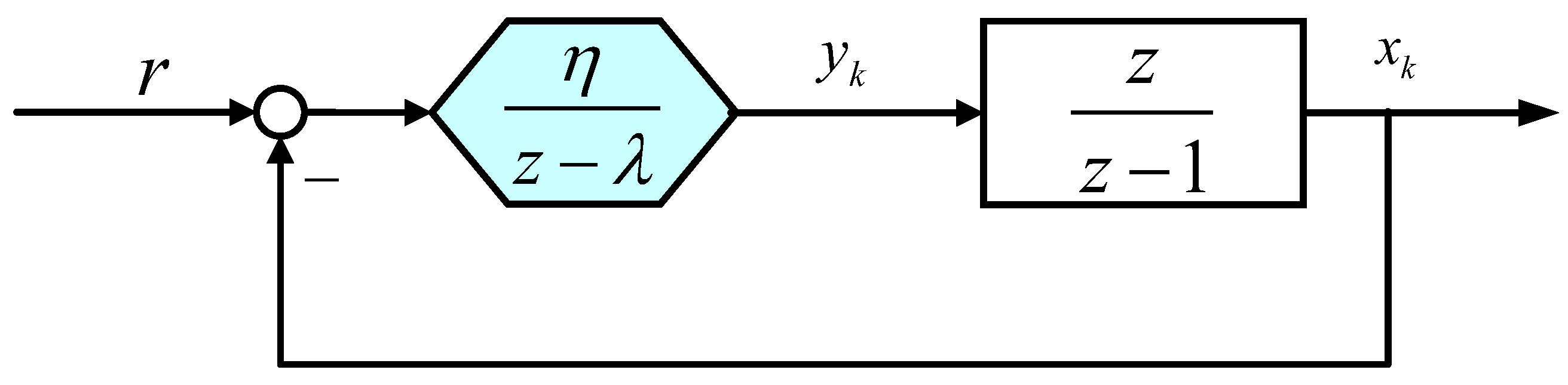
4.2. Euler Discretization of FTGD

In order to apply the FTGD in practice, we will discuss the discrete form of FTGD (13) in this subsection. By using the Euler–Maruyama discretization with step size $\gamma >0$, the discrete form of FTGD (13) with $\alpha =1$ can be derived as

$$\left\{\begin{array}{c}{\theta }_{k+1}=\left(1-\gamma \lambda \right){\theta }_k+\gamma \eta ∥\nabla f\left(x_k\right)∥,\hfill \\ x_{k+1}=x_k-\gamma {\theta }_{k+1}\frac{\nabla f\left(x_k\right)}{∥\nabla f\left(x_k\right)∥}.\hfill \end{array}\right.$$

(20)

To simplify the following discussion, we will ignore the parameter relationship of (13) and (20) and reformulate GD (20) as

$$\left\{\begin{array}{c}{\theta }_{k+1}=\lambda {\theta }_k+\eta ∥\nabla f\left(x_k\right)∥,\hfill \\ x_{k+1}=x_k-{\theta }_{k+1}\frac{\nabla f\left(x_k\right)}{∥\nabla f\left(x_k\right)∥},\hfill \end{array}\right.$$

(21)

where $0<\lambda <1$ and $\eta >0$.

Theorem 2.

For an l-smooth convex function $f\left(x\right)$, algorithm (21) converges to the minimum point asymptotically for $0<\rho <\frac{1-{\lambda }^2}{l}$.

Proof. 

Consider the following Lyapunov function

$$\begin{array}{c}\hfill V_k={∥x_k-x^{*}∥}^2+\frac{{\lambda }^2}{1-{\lambda }^2}{\theta }_k^2,\end{array}$$

(22)

and one has that

$$\begin{array}{cc}\hfill V_{k+1}-V_k=& -2{\theta }_{k+1}\frac{\left(x_k-x^{*}\right)\nabla f\left(x_k\right)}{∥\nabla f\left(x_k\right)∥}+{\theta }_{k+1}^2+\frac{{\lambda }^2}{1-{\lambda }^2}{\theta }_{k+1}^2-\frac{{\lambda }^2}{1-{\lambda }^2}{\theta }_k^2\hfill \\ \hfill =& -2{\theta }_{k+1}\frac{\left(x_k-x^{*}\right)\nabla f\left(x_k\right)}{∥\nabla f\left(x_k\right)∥}+\frac{1}{1-{\lambda }^2}{\theta }_{k+1}^2-\frac{{\lambda }^2}{1-{\lambda }^2}{\theta }_k^2\hfill \\ \hfill \le & -\frac{2}{l}{\theta }_{k+1}∥\nabla f\left(x_k\right)∥+\frac{2\lambda \rho }{1-{\lambda }^2}{\theta }_k∥\nabla f\left(x_k\right)∥+\frac{{\rho }^2}{1-{\lambda }^2}{∥\nabla f\left(x_k\right)∥}^2\hfill \\ \hfill =& \left(\frac{{\rho }^2}{1-{\lambda }^2}-\frac{2\rho }{l}\right){∥\nabla f\left(x_k\right)∥}^2+\left(\frac{2\lambda \rho }{1-{\lambda }^2}-\frac{2\lambda }{l}\right){\theta }_k∥\nabla f\left(x_k\right)∥.\hfill \end{array}$$

If $\rho <\frac{1-{\lambda }^2}{l}$, then $V_{k+1}-V_k\le 0$, and algorithm (21) is asymptotically convergent according to the Lyapunov theorem.    □

4.3. Reset FTGD

Similar to the aforementioned AGDs, FTGD (21) accelerates the convergence speed since the learning rate is always larger than the conventional GD. However, the undesirable overshoot will exist around the minimum point. Then, the reset scheme can be applied to attenuate the overshoot and improve the convergence performance. Different from the aforementioned AGDs, FTGD (21) cannot be directly viewed as a second-order system, but ${\theta }_k$ can be treated as a special control input and set to be zero if the reset condition holds. Reset FTGD can then be formulated in Algorithm 3.

Theorem 3.

For an l-smooth and μ-strongly convex function $f\left(x\right)$, the convergence speed of reset FTGD in Algorithm 3 is linear with $0<\eta <\frac{2}{l+\mu }$.

Algorithm 3 Reset FTGD

Initialize $x_0$, ${\theta }_0$, $\eta$, $\lambda$ for  $k\ge 0$  do    ${\theta }_{k+1}=\lambda {\theta }_k+\eta ∥\nabla f\left(x_k\right)∥$    $x_{k+1}=x_k-{\theta }_{k+1}\frac{\nabla f\left(x_k\right)}{∥\nabla f\left(x_k\right)∥}$    if ${\nabla }^{\mathrm{T}}f\left(x_{k+1}\right)\left(x_{k+1}-x_k\right)>0$ then        ${\theta }_k=0$        ${\theta }_{k+1}=\lambda {\theta }_k+\eta ∥\nabla f\left(x_k\right)∥$        $x_{k+1}=x_k-{\theta }_{k+1}\frac{\nabla f\left(x_k\right)}{∥\nabla f\left(x_k\right)∥}$    end if end for

Proof. 

Suppose the reset operation happens at steps $k_1$, $k_2$, $k_3\cdots$. If linear convergence is proven between any successive two resets, then the proof is completed. In the following, suppose $k_1\le k<k_2$ with start point $x_{k_1}$ and ${\theta }_{k_1}=0$. Additionally, condition ${\nabla }^{T}f\left(x_{k+1}\right)\left(x_{k+1}-x_k\right)\le 0$ holds since there is no reset during this period. Since $f\left(x\right)$ is u-strongly convex, it can be proven that [35]

$$\begin{array}{c}\hfill f\left(x\right)-f\left(x^{*}\right)\le \frac{{∥\nabla f\left(x\right)∥}^2}{2\mu }.\end{array}$$

(23)

Moreover, it is straightforward that

$$\begin{array}{c}\hfill \begin{array}{cc}\hfill ∥x_{k+1}-x_k∥=& \lambda {\theta }_k+\eta ∥\nabla f\left(x_k\right)∥\hfill \\ \hfill =& {\lambda }^2{\theta }_{k-1}+\eta ∥\nabla f\left(x_k\right)∥+\eta \lambda ∥\nabla f\left(x_{k-1}\right)∥\hfill \\ \hfill =& {\lambda }^{k-k_1+1}{\theta }_{k_1}+\eta {\sum }_{i=0}^{k-k_1}{\lambda }^i∥\nabla f\left(x_{k-i}\right)∥.\hfill \end{array}\end{array}$$

(24)

On this basis, the following inequality holds

$$\begin{array}{c}\hfill \begin{array}{cc}\hfill ∥x_{k+1}-x_k∥=& \eta {\sum }_{i=0}^{k-k_1}{\lambda }^i∥\nabla f\left(x_{k-i}\right)∥\hfill \\ \hfill \ge & \eta {\sum }_{i=0}^{k-k_1}{\lambda }^i\sqrt{2\mu \left(f\left(x_k\right)-f\left(x^{*}\right)\right)}\hfill \\ \hfill \ge & \eta \sqrt{2\mu \left(f\left(x_{k_2}\right)-f\left(x^{*}\right)\right)}{\sum }_{i=0}^{k-k_1}{\lambda }^i.\hfill \end{array}\end{array}$$

(25)

Moreover, since $f\left(x\right)$ is u-strongly convex and ${\nabla }^{T}f\left(x_{k+1}\right)\left(x_{k+1}-x_k\right)\le 0$, one has

$$\begin{array}{c}\hfill \begin{array}{cc}\hfill f\left(x_k\right)-f\left(x_{k+1}\right)\ge & {\nabla }^{T}f\left(x_{k+1}\right)\left(x_k-x_{k+1}\right)+\frac{\mu }{2}{∥x_{k+1}-x_k∥}^2\hfill \\ \hfill \ge & \frac{\mu }{2}{∥x_{k+1}-x_k∥}^2\hfill \\ \hfill \ge & {\mu }^2{\eta }^2\left(f\left(x_k\right)-f\left(x^{*}\right)\right){\sum }_{i=0}^{k-k_1}{\lambda }^i.\hfill \end{array}\end{array}$$

(26)

Summing up both sides of (26) from $k_1$ to $k_2$ yields

$$\begin{array}{c}\hfill f\left(x_{k_1}\right)-f\left(x_{k_2}\right)\ge {\mu }^2{\eta }^2\left(f\left(x_k\right)-f\left(x^{*}\right)\right){\displaystyle \sum _{k=k_1}^{k_2-1}}{\displaystyle \sum _{i=0}^{k-k_1}}{\lambda }^i.\end{array}$$

(27)

Furthermore, it is concluded that

$$\begin{array}{c}\hfill \frac{f\left(x_{k_2}\right)-f\left(x^{*}\right)}{f\left(x_{k_1}\right)-f\left(x^{*}\right)}\le \frac{1}{1+{\mu }^2{\eta }^2{\displaystyle \sum _{k=k_1}^{k_2-1}}{\displaystyle \sum _{i=0}^{k-k_1}}{\lambda }^i}.\end{array}$$

(28)

Since $k_2-k_1+1$ must be a finite number, otherwise the linear convergence speed can be followed according to the existing analyses, the mean convergence speed for $k_1\le i\le k_2-1$ can be defined as

$$\begin{array}{c}\hfill {\left[\frac{f\left(x_{i+1}\right)-f\left(x^{*}\right)}{f\left(x_i\right)-f\left(x^{*}\right)}\right]}_{ave}:={\left[\frac{f\left(x_{k_2}\right)-f\left(x^{*}\right)}{f\left(x_{k_1}\right)-f\left(x^{*}\right)}\right]}^{\frac{1}{k_2-k_1+1}}.\end{array}$$

(29)

which indicates a linear convergence. Similar analyses can be applied for any other two successive reset steps.

Additionally, the reset condition (12) implies that the function value decreases constantly until the condition holds. At the step when the reset condition holds, reset MGD is reduced to the conventional GD, and the function value decreases for the learning rate $0<\eta <\frac{2}{l+\mu }$, which indicates the stability of the reset FTGD. □

Remark 3.

•   During the proof process for the linear convergence, the l-smooth property is not required; only the μ-strongly convex property is used. Moreover, condition (23) is exactly the gradient-dominated property.

• As known, for an l-smooth and μ-strongly convex function, the convergence speed for conventional GD can be proven to be linear. The result shown in Theorem 3 is the worst case. Generally, the reset FTGD converges to the minimum point much faster than the conventional GD since the adaptive learning rate is always greater than η.
• Compared with the results in Theorem 2, the stable region of the learning rate for reset FTGD is larger than FTGD without the reset scheme, which improves the stability of FTGD.
• The proposed reset scheme can be applied for other existing optimization algorithms with an adaptive learning rate, such as Adagrad and Adadelta algorithms.

5. Conclusive Discussion

• The reset scheme and fixed-time scheme in system control have been introduced to design high-efficiency GDs for unconstrained convex optimization problems. On the one hand, a general design framework for reset AGDs is given for the first time by using the systematic representation. On the other hand, a novel FTGD with an adaptive learning rate was designed, which has a simpler structure and fewer tuning parameters.
• The proposed algorithms could improve the performance of existing GDs in both convergence rate and stability, where the reset scheme helps attenuate the undesirable overshoot and improve the stability of AGDs, and the fixed-time scheme helps to achieve the non-asymptotic convergence and reach the optimal point in a fixed time.
• The proposed algorithms could be effectively applied for practical usages such as machine learning/deep learning problems. Some instructions for parameter tuning are also given for better practical implementations.

6. Illustrative Examples

In this section, we will validate the fixed-time convergence of FTGD (13) and compare the convergence performance for reset AGDs and reset FTGD. The simulator is MATLAB R2018b, and the simulation step was chosen to be the fixed step with 1 × 10⁻⁵.

Example 1.

In this example, we will show the fixed-time convergence for continuous-time FTGD (13). Consider the quadratic convex function $f(x,y)=\frac{1}{2}{x}^2+2y^2$. Take $\eta =4$, $\lambda =2$, $\alpha =1$ for FTGD (13) and $c_1=c_2=3$, $p_1=3$ and $p_2=\frac{5}{3}$ for FTGD in [22] when simulating. Simulation results with different initial conditions are shown in Figure 3.

• For different initial conditions, fixed-time convergence is achieved by both FTGDs and is smaller than the estimated upper bound (1 s).
• Compared with FTGD in [22], the proposed FTGD (13) not only has fewer tuning parameters but also maintains better robustness to initial conditions where the convergence time is almost the same for different initial conditions as shown in Figure 3a.
• As we have declared before, the exact fixed-time convergence to the minimum point cannot be achieved since FTGD (13) is singular when $\nabla f\left(x\right)=0$, and algorithm (18) can then be applied.

Example 2.

In this example, we will compare the convergence results for different reset AGDs. Consider the quadratic convex function $f\left(x\right)={\displaystyle \sum _{i=1}^n}{a}_i{x}_i^2$, $a_i>0$ and take $a_i=i$ for simplicity. Firstly, we will compare the convergence results for reset AGDs. When simulating, set $n=10$, $\eta =0.01$ and $\lambda =0.8$, and initial conditions are randomly assigned. Results are shown in Figure 4. It is found that for a small learning rate η ($\eta =0.005$ and $\eta =0.01$) that reset MGD and NGD perform similarly, while for a large learning rate ($\eta =0.05$), reset NGD performs much better. However, the stability of reset NGD is worse as shown in Figure 4d, where reset NGD has already reached divergence.

Next, we will compare the performance for reset FTGD with different parameter settings. The results are shown in Figure 5.

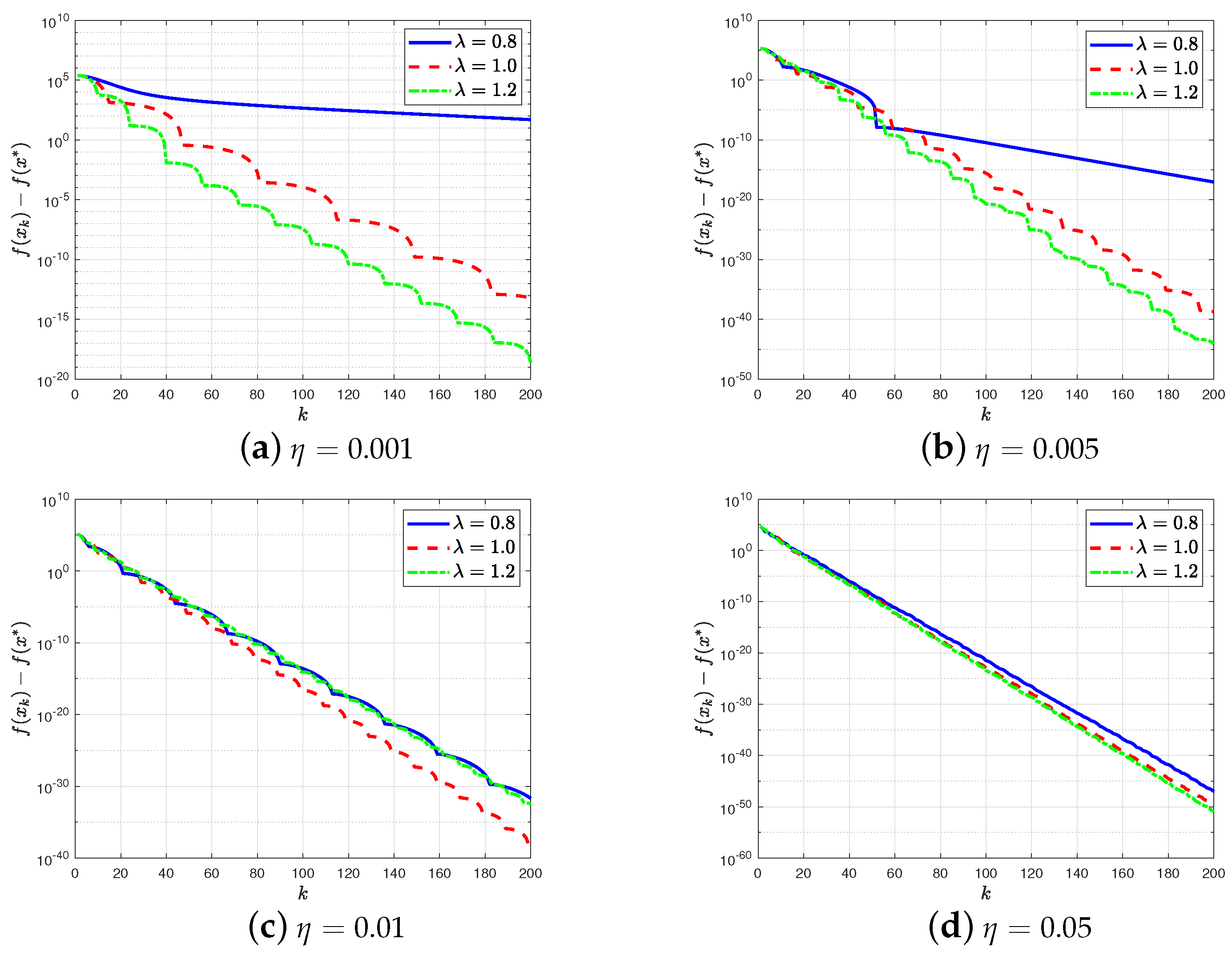
• Unlike the conventional AGDs where λ has to be between 0 and 1, the stability can still be guaranteed for $\lambda \ge 1$. Moreover, for a different learning rate η, a larger λ always performs better, and thus $\lambda =1$ is a good choice for practical usage.
• For a large learning rate ($\eta =0.01$ and $\eta =0.05$), reset FTGD with different λ performs similarly since the reset condition is established almost constantly. Thus, reset FTGD totally reduces to the conventional GD.

Example 3.

In this example, we will consider a special log-sum-exponential function $f\left(x\right)=\log \left({\displaystyle \sum _{i=1}^n}{e}^{a_i{x}^{T}x}\right)$, where $a_i>0$ is randomly assigned in the simulation. When simulating, λ for reset MGD and NGD is set to $0.9$, while λ for reset FTGD is set to $1.0$. Results are shown in Figure 6 and it is observed that

• For different learning rates, reset FTGD always converges the fastest, while reset MGD and reset NGD perform similarly.
• For a small learning rate ($\eta =0.001$), fixed-time convergence of discrete FTGD can be observed in Figure 6a (sharp decaying around $k=100$), which is similar to the result shown in Figure 3b. It is well understood since FTGD (21) has a similar simulation results to its corresponding continuous-time FTGD (20) when the learning rate is sufficiently small.
• Monotone convergence cannot be guaranteed in this example since the mentioned target function is neither l-smooth nor strongly convex, and $f\left(x\right)$ cannot be guaranteed to be decreasing when the reset condition holds.

7. Conclusions and Future Topics

In this paper, the fixed-time scheme and reset scheme are applied to improve the performance of optimization algorithms both in convergence rate and stability. Firstly, a general design framework for reset AGDs is given for the first time by using the systematic representation. Then, a novel adaptive FTGD is proposed, which has fewer tuning parameters and maintains better robustness to initial conditions compared with existing FTGDs. Furthermore, discrete FTGD is given for practical usage, and the reset FTGD is then provided to improve the convergence performance where the linear convergence is rigorously proven. Some instructions on practical implementation and parameter tuning are also provided to make the proposed algorithms more applicable. Finally, dedicated simulation examples are given to validate all the results, and it is found that the reset scheme not only improves the convergence rate but also enhances the stability of the algorithms. However, the proposed algorithms are designed for solving unconstrained convex optimization problems and cannot be directly applied for the stochastic case. Several promising research topics for the future are listed as follows

• Extending the proposed algorithms to the stochastic case;
• Applying the proposed algorithms for practical machine learning problems;
• Combining the developed gradient algorithms with artificial intelligence algorithms.

References

1. Nguyen, B.; Morell, C.; Baets, B.D. Scalable Large-Margin Distance Metric Learning Using Stochastic Gradient Descent. IEEE Trans. Cybern. 2018, 50, 1072–1083. [Google Scholar] [CrossRef] [PubMed]
2. Sun, T.; Tang, K.; Li, D. Gradient Descent Learning with Floats. IEEE Trans. Cybern. 2020, 52, 1763–1771. [Google Scholar] [CrossRef] [PubMed]
3. Cui, F.; Cui, Q.; Song, Y. A Survey on Learning-Based Approaches for Modeling and Classification of Human–Machine Dialog Systems. IEEE Trans. Neural Netw. Learn. Syst. 2020, 32, 1418–1432. [Google Scholar] [CrossRef] [PubMed]
4. Karabayir, I.; Akbilgic, O.; Tas, N. A Novel Learning Algorithm to Optimize Deep Neural Networks: Evolved Gradient Direction Optimizer (EVGO). IEEE Trans. Neural Netw. Learn. Syst. 2021, 23, 685–694. [Google Scholar] [CrossRef] [PubMed]
5. Amari, S.I. Backpropagation and stochastic gradient descent method. Neurocomputing 1993, 5, 185–196. [Google Scholar] [CrossRef]
6. Bottou, L. Large-Scale Machine Learning with Stochastic Gradient Descent. In Proceedings of the Computational Statistics, Pairs, France, 22–27 August 2010; pp. 177–186. [Google Scholar]
7. Qian, N. On the momentum term in gradient descent learning algorithms. Neural Netw. 1999, 12, 145–151. [Google Scholar] [CrossRef]
8. Nesterov, Y.; Polyak, B.T. Cubic regularization of Newton method and its global performance. Math. Program. 2006, 108, 177–205. [Google Scholar] [CrossRef]
9. Yanıkoğlu, İ.; Gorissen, B.L.; den Hertog, D. A survey of adjustable robust optimization. Eur. J. Oper. Res. 2019, 277, 799–813. [Google Scholar] [CrossRef]
10. Sun, X.; Teo, K.L.; Zeng, J.; Liu, L. Robust approximate optimal solutions for nonlinear semi-infinite programming with uncertainty. Optimization 2020, 69, 2109–2129. [Google Scholar] [CrossRef]
11. Sun, X.; Tan, W.; Teo, K.L. Characterizing a Class of Robust Vector Polynomial Optimization via Sum of Squares Conditions. J. Optim. Theory Appl. 2023, 197, 737–764. [Google Scholar] [CrossRef]
12. Kashima, K.; Yamamoto, Y. System theory for numerical analysis. Automatica 2009, 43, 231–236. [Google Scholar]
13. Su, W.; Boyd, S.; Candes, E. A differential equation for modeling Nesterov’s accelerated gradient method: Theory and insights. In Proceedings of the Advances in Neural Information Processing Systems, Montreal, QC, Canada, 8–13 December 2014; pp. 2510–2518. [Google Scholar]
14. Wilson, A.C.; Recht, B.; Jordan, M.I. A Lyapunov analysis of momentum methods in optimization. arXiv 2016, arXiv:1611.02635. [Google Scholar]
15. Wibisono, A.; Wilson, A.C.; Jordan, M.I. A variational perspective on accelerated methods in optimization. Proc. Natl. Acad. Sci. USA 2016, 113, 7351–7358. [Google Scholar] [CrossRef] [PubMed]
16. Hu, B.; Lessard, L. Control interpretations for first-order optimization methods. In Proceedings of the American Control Conference, Seattle, WA, USA, 24–26 May 2017. [Google Scholar]
17. Wu, W.; Jing, X.; Du, W.; Chen, G. Learning dynamics of gradient descent optimization in deep neural networks. Sci. China Inf. Sci. 2021, 64, 150102. [Google Scholar] [CrossRef]
18. Dey, S.; Reich, S. A dynamical system for solving inverse quasi-variational inequalities. Optimization 2023, 1–21. [Google Scholar] [CrossRef]
19. Romero, O.; Benosman, M. Finite-time convergence in continuous-time optimization. In Proceedings of the International Conference on Machine Learning, Virtual, 13–18 July 2020; pp. 8200–8209. [Google Scholar]
20. Polyakov, A. Nonlinear feedback design for fixed-time stabilization of linear control systems. IEEE Trans. Autom. Control. 2011, 57, 2106–2110. [Google Scholar] [CrossRef]
21. Polyakov, A.; Efimov, D.; Perruquetti, W. Finite-time and fixed-time stabilization: Implicit Lyapunov function approach. Automatica 2015, 51, 332–340. [Google Scholar] [CrossRef]
22. Garg, K.; Panagou, D. Fixed-Time Stable Gradient Flows: Applications to Continuous-Time Optimization. IEEE Trans. Autom. Control. 2020, 66, 2002–2015. [Google Scholar] [CrossRef]
23. Wei, Y.; Chen, Y.; Zhao, X.; Cao, J. Analysis and synthesis of gradient algorithms based on fractional-order system theory. IEEE Trans. Syst. Man Cybern. Syst. 2022, 53, 1895–1906. [Google Scholar] [CrossRef]
24. Chen, Y.; Wang, F.; Wang, B. Fixed-time Convergence in Continuous-time Optimization: A Fractional Approach. IEEE Control. Syst. Lett. 2022, 7, 631–635. [Google Scholar] [CrossRef]
25. Firouzbahrami, M.; Nobakhti, A. Cooperative fixed-time/finite-time distributed robust optimization of multi-agent systems. Automatica 2022, 142, 110358. [Google Scholar] [CrossRef]
26. Xu, X.; Yu, Z.; Jiang, H. Fixed-Time Distributed Optimization for Multi-Agent Systems with Input Delays and External Disturbances. Mathematics 2022, 10, 4689. [Google Scholar] [CrossRef]
27. Ogata, K. Discrete-Time Control Systems; Prentice Hall: Hoboken, NJ, USA, 1995. [Google Scholar]
28. O’Donoghue, B.; Candes, E. Adaptive Restart for Accelerated Gradient Schemes. Found. Comput. Math. 2015, 15, 715–732. [Google Scholar] [CrossRef]
29. Kizilkale, C.; Chandrasekaran, S.; Ming, G. Convergence Rate of Restarted Accelerated Gradient. 2017. Available online: https://optimization-online.org/wp-content/uploads/2017/10/6263.pdf (accessed on 16 November 2023).
30. Yang, T.; Lin, Q. Restarted SGD: Beating SGD without Smoothness and/or Strong Convexity. arXiv 2015, arXiv:1512.03107v4. [Google Scholar]
31. Beker, O.; Hollot, C.V.; Chait, Y.; Han, H. Fundamental properties of reset control systems. Automatica 2004, 40, 905–915. [Google Scholar] [CrossRef]
32. Bisoffi, A.; Beerens, R.; Heemels, W.; Nijmeijer, H.; van de Wouw, N.; Zaccarian, L. To stick or to slip: A reset PID control perspective on positioning systems with friction. Annu. Rev. Control 2020, 49, 37–63. [Google Scholar] [CrossRef]
33. Chen, Y.; Wei, Y.; Wang, Y. On 2 types of robust reaching laws. Int. J. Robust Nonlinear Control 2018, 28, 2651–2667. [Google Scholar] [CrossRef]
34. Boyd, S.; Vandenberghe, L. Convex Optimization; Cambridge University Press: Cambridge, UK, 2004. [Google Scholar]
35. Karimi, H.; Nutini, J.; Schmidt, M. Linear convergence of gradient and proximal-gradient methods under the Polyak-Lojasiewicz condition. In Proceedings of the Joint European Conference on Machine Learning and Knowledge Discovery in Databases, Riva, Italy, 19–23 September 2016; Springer: Cham, Switzerland; pp. 795–811. [Google Scholar]
36. Ruder, S. An overview of gradient descent optimization algorithms. arXiv 2016, arXiv:1609.04747v2. [Google Scholar]
Figure 1. Reset control diagram for a second-order system.
Mathematics 11 04704 g001
Figure 2. System responses with/without reset scheme.
Mathematics 11 04704 g002
Figure 3. Comparison of FTGD (13) and FTGD in [22]: (a) convergence results for FTGD (13) (b) convergence results for FTGD in [22].
Mathematics 11 04704 g003
Figure 4. Simulation results for reset AGDs with different learning rates: case 1: reset MGD, case 2: reset NGD.
Mathematics 11 04704 g004
Figure 5. Simulation results for reset FTGD with different η and λ .
Mathematics 11 04704 g005
Figure 6. Simulation results with different learning rates: case 1: reset MGD, case 2: reset NGD, case 3: reset FTGD.
Mathematics 11 04704 g006
Disclaimer/Publisher’s Note: The statements, opinions and data contained in all publications are solely those of the individual author(s) and contributor(s) and not of MDPI and/or the editor(s). MDPI and/or the editor(s) disclaim responsibility for any injury to people or property resulting from any ideas, methods, instructions or products referred to in the content.