Article

Construction of Supplemental Functions for Direct Serendipity and Mixed Finite Elements on Polygons

1
Department of Mathematics, University of Texas at Austin, C1200, Austin, TX 78712-1202, USA
2
Oden Institute for Computational Engineering and Sciences, University of Texas at Austin, C0200, Austin, TX 78712-1229, USA
*
Author to whom correspondence should be addressed.
Mathematics 2023, 11(22), 4663; https://doi.org/10.3390/math11224663
Submission received: 13 October 2023 / Revised: 11 November 2023 / Accepted: 13 November 2023 / Published: 16 November 2023
(This article belongs to the Special Issue Recent Advances in Finite Element Methods with Applications)

Abstract

:
New families of direct serendipity and direct mixed finite elements on general planar, strictly convex polygons were recently defined by the authors. The finite elements of index r are H 1 and H ( div ) conforming, respectively, and approximate optimally to order r + 1 while using the minimal number of degrees of freedom. The shape function space consists of the full set of polynomials defined directly on the element and augmented with a space of supplemental functions. The supplemental functions were constructed as rational functions, which can be difficult to integrate accurately using numerical quadrature rules when the index is high. This can result in a loss of accuracy in certain cases. In this work, we propose alternative ways to construct the supplemental functions on the element as continuous piecewise polynomials. One approach results in supplemental functions that are in H p for any p 1 . We prove the optimal approximation property for these new finite elements. We also perform numerical tests on them, comparing results for the original supplemental functions and the various alternatives. The new piecewise polynomial supplements can be integrated accurately, and therefore show better robustness with respect to the underlying meshes used.

1. Introduction

There has been strong interest in using polygonal and polyhedral meshes when solving certain types of problems via the finite element method. For just a few examples, we note problems in solid mechanics [1,2], elasticity [3,4], fracture mechanics [5,6,7], thin plates [8], shells [9], porous media [10], topology optimization [11,12,13], and finding eigenvalues [14]. In fact, polygonal meshes are an important motivation for the development and use of methods beyond the classic finite element method, which include, for example, the discontinuous Galerkin methods (including weak Galerkin [15] and ultra-weak methods [16,17,18]), mimetic methods [19,20,21], and virtual element methods [22,23,24,25].
Classic conforming finite element methods have also been developed for use on polygonal meshes, and especially for quadrilateral meshes. Approaches taken include the use of maps from reference finite elements [26,27,28], restriction to low order elements [29,30,31,32], the use of macro-elements [33], basis function enrichment [34,35,36], and construction using barycentric coordinates [9,37,38,39]. Ideally, we would have families of conforming finite elements defined for any order of accuracy. These would possess a minimal number of degrees of freedom (DoFs) subject to conformity and accuracy constraints. Finite elements based on the use of non-affine maps from reference finite elements display degraded accuracy. Accuracy is restricted if only low order elements are defined. Macro-elements, basis function enrichment, and the use of barycentric coordinates in higher order cases results in finite elements with an excess number of DoFs.
Families of conforming finite elements defined on polygons that maintain both accuracy and a minimal number of DoFs have appeared recently [40,41,42,43] (as well as some finite elements in three dimensions [44,45,46]). The approach taken is to begin with the space of polynomials P r ( E ) of degree up to r defined directly on the physical element E to achieve accuracy of order r + 1 . To achieve conformity, one then adds in a space of supplemental functions. A basis for the supplemental functions must have certain properties on E , but they must be defined over all of E by filling in the interior. The “supplemental function space” is sometimes called the “filling space”.
In this paper, we discuss the construction of the supplemental functions, in the context of the finite elements developed by the current authors in [43], which are called direct finite elements. Let the element E = E N R 2 be a closed, nondegenerate, convex polygon with N 3 edges. The direct serendipity finite elements of index r 1 are H 1 -conforming and take the form
DS r ( E N ) = P r ( E N ) S r DS ( E N ) ,
where S r DS ( E N ) is the space of supplemental functions. The direct mixed finite elements are H ( div ) -conforming and take two forms,
V r r ( E N ) = P r 2 ( E N ) x P ˜ r ( E N ) S r V ( E N ) , V r r 1 ( E N ) = P r 2 ( E N ) S r V ( E N ) ,
for full ( r 0 ) and reduced ( r 1 ) H ( div ) -approximation, respectively, where P ˜ r ( E N ) are the homogeneous polynomials of (exact) degree r. These two finite elements are related to each other by the finite element exterior calculus [47] through the de Rham complex
R H 1 curl H ( div ) div L 2 0 ,
resulting in, for s = r 1 , r ( s 0 ) ,
R DS r + 1 ( E N ) curl V r s ( E N ) div P s ( E N ) 0 .
The consequence is that
V r r ( E N ) = curl D S r + 1 ( E N ) x P r , V r r 1 ( E N ) = curl DS r + 1 ( E N ) x P r 1 ,
and, therefore,
S r V ( E N ) = curl S r + 1 DS ( E N ) .
The original construction of supplemental functions made use of rational functions (see (21)), which are difficult to numerically integrate accurately. As a consequence, when solving a partial differential equation using direct finite elements, the quadrature error may be significant, leading to poor overall approximation of the solution. This was observed in [43], although in that paper, the degradation in the approximation was attributed to poor mesh quality. While mesh quality remains an important ingredient in finite element analysis, quadrature approximation is also a critical component, especially for high order methods.
In this work, we introduce two constructions of the supplemental functions S r DS ( E N ) which involve using continuous piecewise polynomials. Such constructions are motivated by the work of Kuznetsov and Repin [33], and suggested by the work of Cockburn and Fu [41]. These new supplemental functions can then be accurately integrated by quadrature rules. (A similar, but more complex, construction in three dimensions for cuboidal hexahedra is discussed in [46]).
In the next two sections we present some basic notation and review the general definition of the original direct serendipity and direct mixed finite elements, which have supplemental functions that are C -smooth. Our new families of direct finite elements based on piecewise continuous supplemental functions are given in Section 4. We give two constructions of the supplemental functions, so that one set lies in H 1 and the other in H p for any integer p 1 . The approximation properties of these new direct finite elements are given in Section 5. The results are optimal, up to the bounding constant. The proof follows that given in [43], and we concentrate on the modifications that are required to handle the new supplements. In Section 6, we present numerical tests that compare the errors and convergence rates of the new and original direct finite elements. We conclude the paper in Section 7.

2. Notation

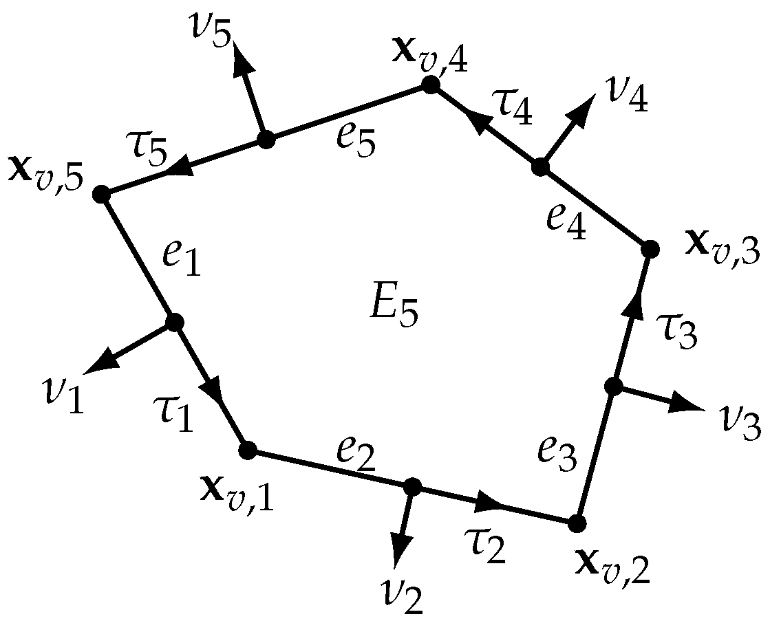
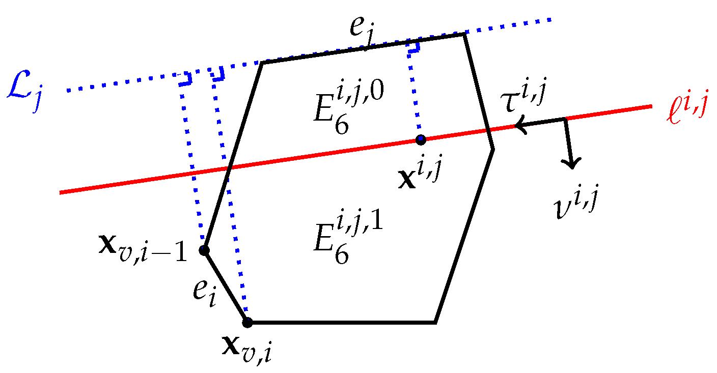
We choose to identify the edges and vertices of E N adjacently in the counterclockwise direction, as depicted in Figure 1 (throughout the paper, we interpret indices modulo N). Let the edges of E N be denoted e i , i = 1 , 2 , , N , and the vertices be x v , i = e i e i + 1 . Let ν i denote the unit outer normal to edge e i , and let τ i denote the unit tangent vector of e i oriented in the counterclockwise direction, for i = 1 , 2 , , N .
For any two distinct points y 1 and y 2 , let L [ y 1 , y 2 ] be the line passing through y 1 and y 2 , and take ν [ y 1 , y 2 ] to be the unit vector normal to this line interpreted as going from y 1 to y 2 and then spinning 90 degrees in the clockwise direction (i.e., pointing to the right). Then we define a linear polynomial giving the signed distance of x to L [ y 1 , y 2 ] as
λ [ y 1 , y 2 ] ( x ) = ( x y 2 ) · ν [ y 1 , y 2 ] .
To simplify the notation for linear functions that will be used throughout the paper, let L i = L [ x v , i 1 , x v , i ] be the line containing edge e i and let λ i ( x ) give the distance of x R 2 to edge e i opposite the normal direction, i.e.,
λ i ( x ) = λ [ x v , i 1 , x v , i ] ( x ) = ( x x v , i ) · ν i , i = 1 , 2 , , N .
These functions are strictly positive in the interior of E N , and λ i vanishes on the edge e i .

3. Direct Serendipity and Mixed Finite Elements

The general development of direct serendipity and mixed finite elements is given in [43]. The definition of the supplemental space S r DS ( E N ) in (1) is key to the construction. For completeness, we review the definitions of these direct finite elements here.
When N = 3 (triangles), the direct serendipity supplemental space S r DS ( E 3 ) is empty. When N 4 and 1 r < N 2 , the direct serendipity spaces DS r ( E N ) are defined as subspaces of DS N 2 ( E N ) by the rule
DS r ( E N ) = φ DS N 2 ( E N ) : φ | e P r ( e ) for all edges e of E N .
Therefore, we only need to understand S r DS ( E N ) for r N 2 and N 4 .
To define the supplemental basis functions, two series of choices must be made for each i , j such that 1 i < j N and 2 j i N 2 (i.e., e i and e j are nonadjacent edges). First, as shown in Figure 2, one must choose two distinct points x i , j 1 L i and x i , j 2 L j that avoid the intersection point x i , j = L i L j , if it exists. Then let
λ i , j ( x ) = λ [ x i , j 1 , x i , j 2 ] ( x ) = ( x x i , j 2 ) · ν i , j , ν i , j = ν [ x i , j 1 , x i , j 2 ] ,
be the linear function associated to the line L i , j = L [ x i , j 1 , x i , j 2 ] . Second, R i , j must be chosen to satisfy
R i , j ( x ) | e i = 1 , R i , j ( x ) | e j = 1 .
The supplemental space for r N 2 2 is of the form
S r DS ( E N ) = span ϕ s , i , j : 1 i < j N , 2 j i N 2 ,
ϕ s , i , j = k i , j λ k λ i , j r N + 2 R i , j .

3.1. Direct Serendipity Finite Elements

Every shape function of the direct serendipity finite element DS r ( E N ) is a sum of a polynomial and a linear combination of the supplemental functions, as in (1). To implement them, one must define the DoFs. For example, for ψ DS r ( E N ) , one can take
ψ ( x v , i ) , i = 1 , 2 , , N ,
e i ψ p d σ , p P r 2 ( e i ) , i = 1 , 2 , , N ,
E N ψ q d x , q P r N ( E N ) ,
where d σ is the one dimensional surface measure. Alternatively, one can use nodal DoFs (i.e., evaluation at a node point) in place of (15) and/or (16). For the former, on each edge e i , its corresponding edge nodes are r 1 points such that they, along with the two vertices, are equally distributed on e i . For the latter, the interior cell nodes can be set to be the Lagrange nodes of order r N of a triangle that lies strictly inside E N .
The basis of DS r ( E N ) corresponding to the DoFs can be constructed. Given a computational mesh of convex polygons T h over a domain Ω , the basis can be simply pieced together to form a global H 1 -conforming basis of the space DS r ( Ω ) H 1 ( Ω ) .

3.2. Direct Mixed Finite Elements

As discussed in the introduction, full, V r r ( E N ) , and reduced, V r r 1 ( E N ) , H ( div ) -approximating mixed finite element spaces follow from a de Rham complex (3), where the direct serendipity finite elements serve as the precursor (4). The supplemental space is related to S r + 1 DS ( E N ) by the simple Formula (6).
The DoFs for these spaces (with s = r 0 or s = r 1 0 ) can be taken to be
e i v · ν i p d σ , p P r ( e i ) , i = 1 , 2 , , N ,
E N v · q d x , q P s ( E N ) , q not constant ,
E N v · ψ d x , ψ B r V ( E N ) , if r N 1 ,
where the H 1 ( E N ) and H ( div ; E N ) bubble functions, for r N 1 , are
B r + 1 ( E N ) = λ 1 λ 2 λ N P r N + 1 ( E N ) and B r V ( E N ) = curl B r + 1 ( E N ) .
Given the mesh T h over Ω , one constructs the basis and the H ( div ) -conforming global space V r s ( Ω ) H ( div ) (see [43] for details). As an alternative, when solving partial differential equations, one can use the hybrid form of the method [48], which does not require the construction of global basis functions.

4. Piecewise Continuous Supplements

In [43], R i , j satisfying (11) on E N , for 1 i < j N , 2 j i N 2 , was taken to be the simple rational function
R i , j rational ( x ) = λ i ( x ) λ j ( x ) λ i ( x ) + λ j ( x ) .
These rational functions are smooth over the element. We now give new direct serendipity and mixed finite elements by providing an alternate construction of R i , j as a piecewise continuous polynomial defined over a sub-partition of E N . We present two strategies, the first of which is convenient for the construction of continuous supplemental functions in H 1 ( E N ) , and the second for constructing smoother supplemental functions in H p ( E N ) for integer p 1 .

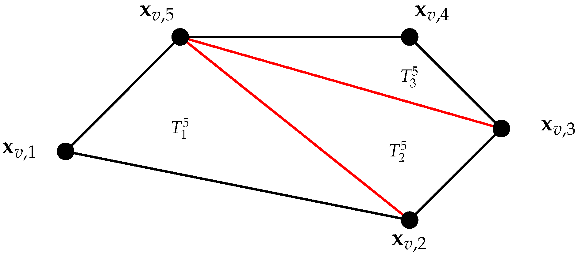
4.1. Supplemental Functions in H 1 ( E N )

Our first strategy for constructing R i , j requires a sub-triangulation of the element E N , and we present two natural choices. The first sub-triangulation is depicted in Figure 3 and denoted as T n ( E N ) . One picks a vertex x v , n and divides E N into N 2 sub-triangles. The sub-triangles are T m n with vertices x v , n , x v , m , and x v , m + 1 , where m = n + 1 , , n + N 2 
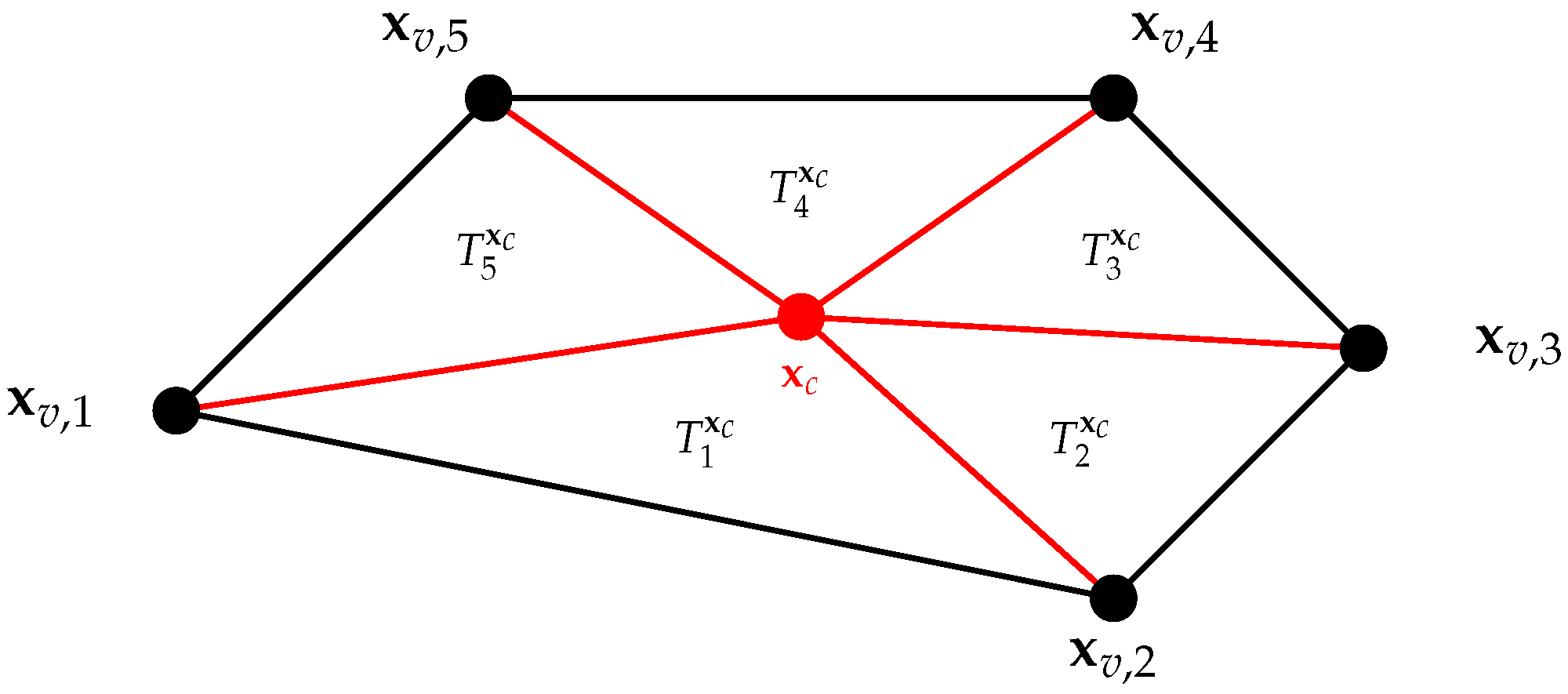
. For the second sub-triangulation, depicted in Figure 4 and denoted as T x c ( E N ) , one picks a point x c in the interior of E N and divides it into N sub-triangles. Now the sub-triangles are T m x c with vertices x c , x v , m , and x v , m + 1 , where m = 1 , 2 , , N . We use the centroid of the element for x c .
Let the piecewise polynomial function space of degree s corresponding to each sub-triangulation be
P s ( T n ( E N ) ) = { f C 0 ( E ) | f | T m n P s ( T m n ) , m = n + 1 , , n + N 2 } ,
P s ( T x c ( E N ) ) = { f C 0 ( E ) | f | T m x c P s ( T m x c ) , m = 1 , 2 , , N } .
We construct R i , j in P 1 ( T n ( E N ) ) or P 1 ( T x c ( E N ) ) , depending on which of the two sub-triangulations is used, such that
R i , j | e i = 1 , R i , j | e j = 1 , R i , j | v k = 0 , k i 1 , i , j 1 , j .
by using interpolation at the vertices of the sub-triangles. If the sub-triangulation is chosen to be T n ( E N ) , the restrictions (24) uniquely specify all the vertex values. However, if the triangulation is T x c ( E N ) , the center value is not determined, so we assign R i , j ( x c ) = 0 .
Our construction has R i , j being 1 on e i and 1 on e j as required by (11). Moreover, R i , j H 1 ( E N ) . After constructing the supplemental functions in (13) with this R i , j , each ϕ s , i , j is in P r + 1 ( T n ( E N ) ) or P r + 1 ( T x c ( E N ) ) , and therefore also in H 1 ( E N ) .

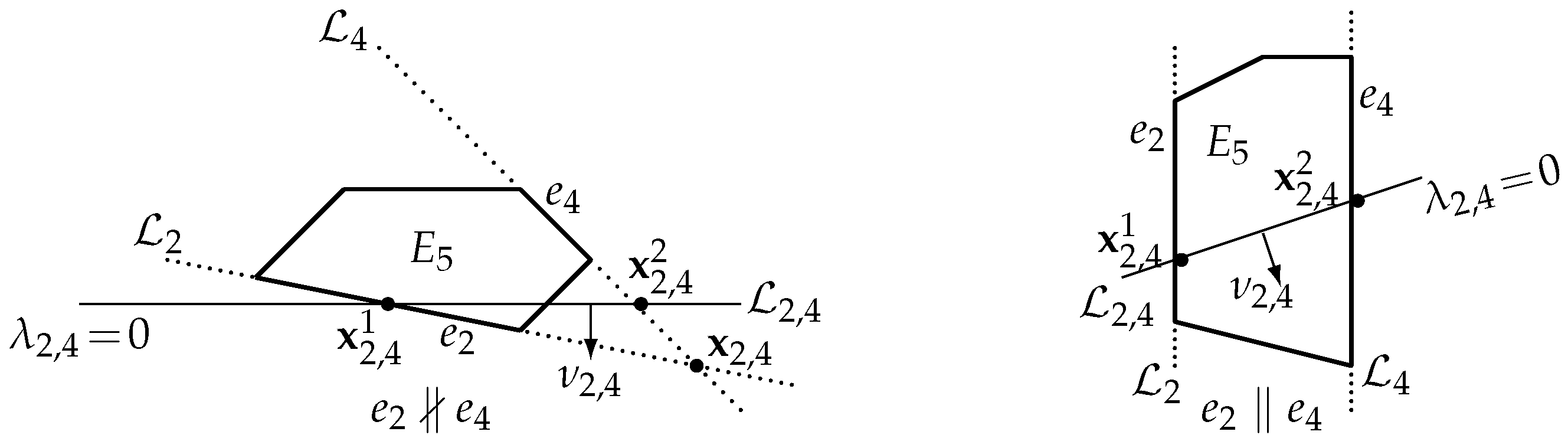
4.2. Supplemental Functions in H p ( E N )

We now present the second of our two strategies for constructing R i , j for two nonadjacent edges e i and e j . Recall that λ k ( x ) is the linear polynomial giving the (signed) distance to the line L k extending edge e k . When e i and e j are parallel, we simply define R i , j as the linear polynomial
R i , j = λ i λ j λ i ( x v , j ) .
When e i and e j are not parallel, we first define a sub-partition of E N by adding a single extra line i , j through a point x i , j as depicted in Figure 5. The point x i , j is chosen so that it is closer to L j than the endpoints of e i , i.e.,
λ j ( x i , j ) min { λ j ( x v , i 1 ) , λ j ( x v , i ) } .
The line i , j passes through x i , j and is parallel to e j . This line divides E N into E N i , j , 1 near e i and E N i , j , 0 near e j , i.e.,
E N i , j , 1 = E N { x | λ j ( x ) λ j ( x i , j ) } ,
E N i , j , 0 = E N { x | λ j ( x ) < λ j ( x i , j ) } .
Let ν i , j = ν j be the unit normal vector of i , j pointing into E N i , j , 1 , and let τ i , j = τ j be a unit tangent vector.
We next construct the function ρ i , j , which is 1 on edge e i and 0 on edge e j . It is defined piecewise on the sub-partition of E N as
ρ i , j ( x ) = 1 , x E N i , j , 1 , 1 1 λ j ( x ) λ j ( x i , j ) p , x E N i , j , 0 ,
where p 1 is an integer. The function is continuous, since λ j ( x ) = λ j ( x i , j ) on i , j implies that ρ i , j | i , j = 1 in either case of the definition. Moreover, in the tangential direction,
ρ i , j τ i , j | i , j = 0 ,
and, in the normal direction,
ρ i , j ν i , j ( x ) = 0 , x E N i , j , 1 , p λ j ( x i , j ) 1 λ j ( x ) λ j ( x i , j ) p 1 , x E N i , j , 0 ,
which is continuous for p > 1 , so ρ i , j C 1 ( E N ) . By iterating the argument, we have that ρ i , j C p 1 ( E N ) and so also in H p ( E N ) for p > 1 . If p = 1 , ρ i , j is continuous, so it is in H 1 ( E N ) .
Finally, after constructing both ρ i , j and ρ j , i , we define
R i , j = ρ j , i ρ i , j ,
which is 1 on e i , 1 on e j . Moreover, R i , j H p ( E N ) . The supplemental functions in (13) constructed with this R i , j lie in H p ( E N ) .
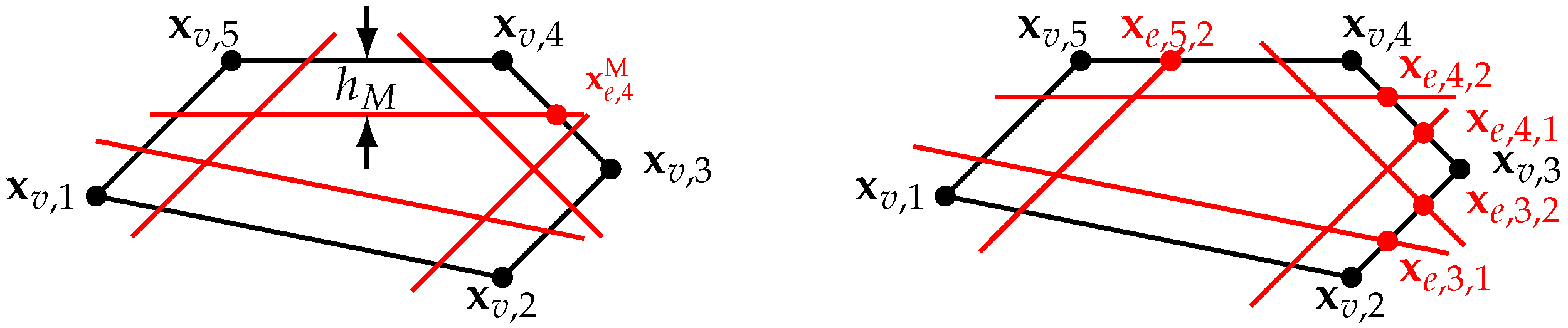
We end this section with two specific examples, using the sub-partitions shown in Figure 6, which divide E N by N lines. The first example has a sub-partition based on the midpoints x e , i M of the edges e i , i = 1 , 2 , , N , and gives rise to the spaces denoted DS r M ( E N ) and V r M , s ( E N ) . We compute the minimal distance of the midpoints to the edges, i.e.,
h M = min 1 i N , k = i ± 1 λ i ( x e , k M ) .
Then for any two non parallel and nonadjacent edges e i and e j , simply take the partition line i , j to be the line parallel to e j that is the fixed distance h M > 0 away and intersects E N .
The second specific example uses a sub-partition based on trisecting each edge, resulting in the points, for edge e i , being denoted counterclockwise as x e , i , k for k = 1 , 2 , i = 1 , 2 , , N . In this case, we simply take x i , j to be the closest of these points to L j , omitting x e , j , 1 and x e , j , 2 . We denote the resulting spaces DS r T ( E N ) and V r T , s ( E N ) .

5. Approximation Properties

We discuss now the global approximation properties for our direct finite element spaces. The results of [43] do not directly apply here because there it was assumed that the functions R i , j are smooth on the element. Consider a collection of meshes T h of convex polygons partitioning a domain Ω , where h > 0 is the maximal element diameter.
We need to make the usual assumption that our collection of meshes is uniformly shape regular [49] (pp. 104–105). For any E N T h , let h E N be its diameter. Denote by T i , i = 1 , 2 , , N ( N 1 ) ( N 2 ) / 6 , the sub-triangle of E N with vertices being three of the N vertices of E N , and define
ρ E N = 2 min 1 i N ( N 1 ) ( N 2 ) / 6 { diameter of the largest circle inscribed in T i } .
The shape regularity parameter of the single mesh T h is
σ T h = min E N T h ρ E N h E N .
Assumption 1. 
The collection of meshes { T h } h > 0 is  uniformly shape regular.  That is, the shape regularity parameters are bounded below by a positive constant: there exists σ > 0 , independent of T h and h > 0 , such that the ratio
ρ E N h E N σ > 0 for all E N T h , h > 0 .
We also require some mild restrictions on the construction of S r DS ( E N ) .
Assumption 2. 
For every E N T h , assume that the functions of S r DS ( E N ) are constructed using λ i , j such that the zero set L i , j intersects e i and e j . Moreover, suppose that R i , j H p ( E N ) for some p 1 and that the sub-partitions introduced in Section 4 for their construction depend continuously on the vertices of E N .
The continuous dependence requirement of the sub-partitions is met if we systematically choose the points x c in Section 4.1 (say as the centroid) and x i , j satisfying (26) in Section 4.2 (say be taking x i , j as the closer endpoint of e i to L j , or so that λ j ( x i , j ) = 1 2 min { λ j ( x v , i 1 ) , λ j ( x v , i ) } ).
We state first the approximation result for DS r ( Ω ) .
Theorem 1. 
Let r 1 , 1 p , and > 1 / p (or 1 if p = 1 ). If Assumptions 1 and 2 hold (so the basis functions are in H p on each element), then there exists a constant C > 0 , such that for all functions v W , p ( Ω ) ,
inf v h DS r ( Ω ) v v h W m , p ( Ω ) C h m v W , p ( Ω ) , 0 r + 1 , m = 0 , 1 .
Proof. 
The methodology of the proof follows [42,43]. The key difference is that we must relax the smoothness requirement made on the supplemental functions. We highlight the differences, and leave the reader to consult [42,43] for some of the details.
Given a mesh T h , we construct an interpolation operator I h r : W p l ( Ω ) DS r as a generalization of that defined in [50]. To do so, we use a nodal set of DoFs for the finite elements, and identify global nodal points a i , i = 1 , 2 , , dim DS r . These nodal points must be chosen systematically with respect to the vertices of the mesh, so they depend continuously on them. The global nodal basis function for a i is denoted φ i .
A geometry object K i is associated to each a i . If a i lies in the interior of some element, we choose the element to be K i . Otherwise, we choose an edge containing a i to be K i , where we additionally ask that K i Ω if a i Ω . We use these to define the dual basis ψ i with respect to L 2 ( K i ) , i = 1 , 2 , , dim DS r . The corresponding interpolation operator I h r : W p l ( Ω ) DS r is then
I h r v ( x ) = i = 1 dim DS r K i ψ i ( y ) v ( y ) d y φ i ( x ) .
There are two essential steps towards showing the approximation property. First, the nodal basis functions are bounded,
max 1 i dim DS r ( Ω ) max E T h | | φ i | | W q m ( E ) C ,
and, second, the dual basis functions are bounded up to a scaling factor,
| | ψ i | | L ( K i ) C h K i dim K i .
We show the necessary boundedness by mapping the elements and using a continuity and compactness argument.
As depicted in Figure 7, to each element E N , we associate a regular polygon (equilateral and equiangular) E ^ N . We can then define a map F E N : E ^ N E N as a composition of a map that changes the geometry but not the size to E ˜ N , and then a scaling map (see [43] for precise details).
Define the nodal basis functions φ i E ˜ N on E ˜ N . It is enough to show the boundedness of their W q m norms. Although they are no longer smooth functions, compared to [42,43], they are continuous on E ˜ N , and smooth on all the subregions generated by the sub-partition. Moreover, by assumption the sub-partition is required to depend continuously on the vertices of E ˜ N . Therefore, φ i E ˜ N will still depend continuously on x ^ = F E ˜ N 1 ( x ˜ ) and the vertices of E ˜ N , which vary in a compact set. We conclude that the nodal basis functions are bounded in W q m norm. The boundedness of ψ i in the L norm can be shown in a similar way. □
For the mixed finite elements, we have the following result, wherein we see projection operators π : H ( div ; Ω ) ( L 2 + ϵ ( Ω ) ) 2 V r s , s = r 1 , r , where ϵ > 0 , and P W s , the L 2 -orthogonal projection operator onto W s = · V r s .
Theorem 2. 
Let r = s 0 or r 1 , s = r 1 . If Assumptions 1 and 2 hold, then there is a constant C > 0 , such that
v π v L 2 ( Ω ) C v H k ( Ω ) h k , k = 1 , , r + 1 ,
p P W s p L 2 ( Ω ) C p H k ( Ω ) h k , k = 0 , 1 , , s + 1 ,
· ( v π v ) L 2 ( Ω ) C · v H k ( Ω ) h k , k = 0 , 1 , , s + 1 ,
where s = r 1 0 and s = r 1 for reduced and full H ( div ) -approximation, respectively. Moreover, the discrete inf-sup condition
sup v h V r s ( w h , · v h ) v h H ( div ) γ w h L 2 ( Ω ) , w h W s ,
holds for some γ > 0 independent of h > 0 .
For the proof, we define the projection operator π by piecing together local operators π E that are defined in terms of the DoFs (17)–(19). The approximation properties given in [42,43] hold with a similar proof, using now that the subregions generated by the sub-partition depend continuously on the vertices of the element.

6. Numerical Results

We present numerical experiments for our new finite elements as applied to Poisson’s equation
· ( p ) = f in Ω ,
p = 0 on Ω ,
where f L 2 ( Ω ) . The corresponding weak form finds p H 0 1 ( Ω ) such that
( p , q ) = ( f , q ) , q H 0 1 ( Ω ) ,
where ( · , · ) is the L 2 ( Ω ) inner product. Setting
u = p ,
we have the mixed weak form, which finds u H ( div ; Ω ) and p L 2 ( Ω ) such that
( u , v ) ( p , · v ) = 0 , v H ( div ; Ω ) ,
( · u , w ) = ( f , w ) , w L 2 ( Ω ) .
These weak forms naturally give rise to finite element approximations. According to Theorems 1 and 2, the following convergence analysis holds by a standard argument [27,51].
Theorem 3. 
If Assumptions 1 and 2 hold, then there exists a constant C > 0 , independent of T h and h > 0 , such that for r 1 ,
p p h m , Ω C h + 1 m | p | + 1 , Ω , = 0 , 1 , , r , m = 0 , 1 ,
where p h DS r ( Ω ) H 0 1 ( Ω ) approximates (47). Moreover, with r = s 0 or r 1 , s = r 1 ,
u u h 0 , Ω C u k , Ω h k , k = 1 , , r + 1 ,
p p h 0 , Ω C u k , Ω h k , k = 1 , , s + 1 ,
· ( u u h ) 0 , Ω C · u k , Ω h k , k = 0 , 1 , , s + 1 ,
where ( u h , p h ) V r s   ×   W s approximates (49) and (50).
We perform our tests on a unit square domain Ω = [ 0 , 1 ] 2 , and take the source term f ( x ) = 2 π 2 sin ( π x 1 ) sin ( π x 2 ) , so the exact solution is u ( x 1 , x 2 ) = sin ( π x 1 ) sin ( π x 2 ) . We consider five types of supplemental spaces. The original direct serendipity and mixed finite element spaces will be denoted DS r R and V r R , s , respectively. These use supplements based on the rational functions (21).
For the H 1 supplemental functions introduced in Section 4.1, there are two varieties. Denote the space using supplemental functions that are constructed based on the vertex sub-triangulation as DS r V and its corresponding mixed spaces as V r V , s , and those based on the center point sub-triangulation as DS r C and V r C , s , respectively. The spaces based on the H p supplements were described in Section 4.2 and denoted DS r M , V r M , s and DS r T , V r T , s .

6.1. The Meshes Used

Approximate solutions are computed on a sequence of Voronoi meshes T h 2 generated by the package PolyMesher [52]. Each mesh has n 2 elements, which are generated with n 2 random initial seeds and up to 10 4 smoothing iterations to improve the shape regularity.
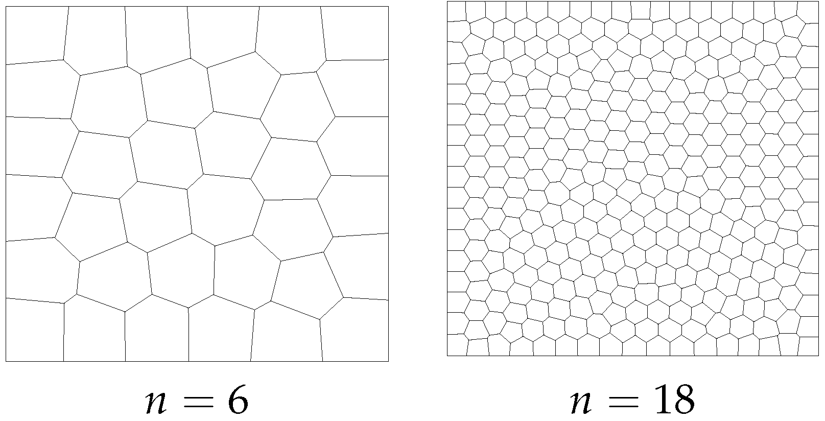
For comparison to the results appearing in [43], we use the same mesh sequence T h 2 with n = 6 , 10, 14, 18, and 22. We show the meshes for n = 6 and n = 18 in Figure 8. The shape regularity parameters are given in Table 1. Note that the n = 10 and n = 18 meshes are the least regular.
In [43] it was observed numerically that the n = 18 mesh performed well for the original direct finite elements (using rational supplemental functions) when r = 2 , 3 , 4 , but had a degraded convergence rate when r = 5 . The problem was resolved by removing short edges from the n = 18 mesh. However, as we will see in this section, the problem is actually due to inaccurate numerical quadrature of the rational supplemental functions, which only showed up in those tests for the more refined mesh (i.e., not n = 10 ) and higher values of r.

6.2. Results for Direct Serendipity Spaces

We present and compare the results of the numerical tests performed for DS r R , DS r V , DS r C , DS r M , and DS r T , where r = 2 , 3 , 4 , 5 . We take p = 1 in Section 4.2 for the construction of DS r M and DS r T , because it gives better results than a larger p in most cases. According to Theorem 3, we expect all those spaces to have the convergence rates r + 1 for L 2 errors and r for H 1 -seminorm errors. As Table 2 and Table 3 suggests, the convergence rates at n = 10 , 14 , 22 for DS r R are all slightly better than optimal in this test. However, we can observe a slower convergence rate at n = 18 for DS r R . (We interject that convergence rates are computed as improvement from the previous mesh in our sequence.)
In Table 4, we compare the results for the n = 18 mesh of DS r R , DS r V , DS r C , DS r M , and DS r T . On the one hand, the results suggest that the new spaces are all approximately optimal for r = 5 , which is an obvious improvement compared to DS 5 R . On the other hand, the errors for r = 2 , 3 , 4 of the new spaces are slightly worse than those of DS r R , and among all the new spaces, DS r C has the best performance in error. We conclude that DS r C shows the best overall performance among all the spaces considered.
We suggest that the reason for such an observation is that the dominant errors for r = 5 are from the numerical quadrature applied to the integration of rational functions, especially on the elements that are less shape regular. However, for r = 2 , 3 , 4 , the new supplements, as piecewise polynomials, cannot approximate the shape of a smooth function as well as the original rational supplements, especially those from DS r M and DS r T , of which R i , j for e i e j are flat in the middle and oscillate near the boundary. In contrast, the supplements from DS r V and DS r C are more reasonably shaped, and those from DS r C are better since its partition has sub-triangles that are more shape regular (as was shown in Figure 3 and Figure 4). This argument is also supported by the observation that the results are usually worse if we take larger p for DS r M and DS r T , where the shape of the supplements are even worse.

6.3. Results for Direct Mixed Spaces

We perform numerical tests for V r R , s , V r V , s , V r C , s , V r M , s , V r T , s , for the full H ( div ) -approximation spaces where r = s = 0 , 1 , 2 , 3 , and the reduced H ( div ) -approximation spaces where r = 1 , 2 , 3 , and s = r 1 . Since those mixed spaces are constructed from corresponding direct serendipity spaces DS r + 1 , it is natural that we find the comparison of the results similar to the small r cases discussed in Section 6.2. For all the spaces, we can observe the convergence rates approximately optimal in general but the errors are slightly worse for n = 18 , especially when r = s = 3 , as shown in Table 5 and Table 6. All spaces perform similarly well, although V r R , s usually performs best in these tests. Among the new spaces, V r C , s performs a bit better, and it gives results close to those of V r R , s . For reference, we provide the numerical results for V r C , s in Table 7 and Table 8.

7. Conclusions

We reviewed the construction of direct serendipity and mixed finite elements on non-degenerate, planar convex polygons. The direct serendipity finite element spaces are of the form
DS r ( E N ) = P r ( E N ) S r DS ( E N ) .
The full and reduced H ( div ) -approximation mixed finite element spaces are obtained from a de Rham complex, where the direct serendipity finite elements serve as a precursor. The mixed spaces are of the form
V r r ( E N ) = P r 2 ( E N ) x P ˜ r ( E N ) S r V ( E N ) , V r r 1 ( E N ) = P r 2 ( E N ) S r V ( E N ) ,
where
S r V ( E N ) = curl S r + 1 DS ( E N ) .
We presented two approaches to construct the supplemental functions in S r DS ( E N ) as piecewise polynomials. The first approach divides a polygonal element E N into sub-triangles, and constructs the supplements as continuous piecewise polynomials that lie in H 1 ( E N ) . The second approach has a more complicated subdivision of E N that needs to be treated carefully. However, it provides a framework for constructing supplements that lie in H p ( E N ) for any p 1 .
The approximation properties of the new finite elements were proved under the regularity assumption of the mesh sequences and some mild restrictions on the construction.
We performed numerical tests on a randomly generated mesh sequence and compared results for five different ways of constructing the supplemental functions, including the original construction using smooth but rational functions. The comparison suggested that it is better to use the piecewise polynomial supplements rather than the rational supplements for higher order r. Although the rational supplements are smooth and so tend to approximate better, noticeable errors could be seen due to inaccurate numerical integration, especially on meshes with short edges. Among the new spaces, it was found that the spaces with supplements based on the center point sub-triangulation (23) performed best.

Author Contributions

Conceptualization, T.A. and C.W.; Methodology, T.A. and C.W.; Software, T.A. and C.W.; Writing—original draft, T.A. and C.W.; Writing—review & editing, T.A. and C.W.; Funding acquisition, T.A. Both authors contributed about equally to the work. All authors have read and agreed to the published version of the manuscript.

Funding

This research was funded by U.S. National Science Foundation grant number DMS-2111159.

Data Availability Statement

All pertinent data generated or analyzed during this study are included in this published article. Supporting data omitted from the article are available from the corresponding author on reasonable request.

Conflicts of Interest

The authors declare no conflict of interest.

References

  1. Bishop, J.E. A displacement-based finite element formulation for general polyhedra using harmonic shape functions. Int. J. Numer. Methods Eng. 2014, 97, 1–31. [Google Scholar] [CrossRef]
  2. Bishop, J.E.; Sukumar, N. Polyhedral finite elements for nonlinear solid mechanics using tetrahedral subdivisions and dual-cell aggregation. Comput. Aided Geom. Des. 2020, 77, 101812. [Google Scholar] [CrossRef]
  3. Tabarraei, A.; Sukumar, N. Application of polygonal finite elements in linear elasticity. Int. J. Comput. Methods 2006, 3, 503–529. [Google Scholar] [CrossRef]
  4. Paz, J.D.M. PolyDPG: A Discontinuous Petroz-Galerkin Methodology for Polytopal Meshes with Applications to Elasticity. Ph.D. Thesis, University of Texas at Austin, Austin, TX, USA, 2020. [Google Scholar]
  5. Spring, D.W.; Leon, S.E.; Paulino, G.H. Unstructured polygonal meshes with adaptive refinement for the numerical simulation of dynamic cohesive fracture. Intl. J. Fract. 2014, 189, 33–57. [Google Scholar] [CrossRef]
  6. Chi, H.; Talischi, C.; Lopez-Pamies, O.; Paulino, G. Polygonal finite elements for finite elasticity. Int. J. Numer. Methods Eng. 2015, 101, 305–328. [Google Scholar] [CrossRef]
  7. Bishop, J.E. Applications of Polyhedral Finite Elements in Solid Mechanics. In Generalized Barycentric Coordinates in Computer Graphics and Computational Mechanics; CRC Press: Boca Raton, FL, USA, 2017; pp. 179–196. [Google Scholar]
  8. Di Pietro, D.; Droniou, J. A fully discrete plates complex on polygonal meshes with application to the Kirchhoff–Love problem. Math. Comput. 2023, 92, 51–77. [Google Scholar] [CrossRef]
  9. Ho-Nguyen-Tan, T.; Kim, H.G. Polygonal shell elements with assumed transverse shear and membrane strains. Comput. Methods Appl. Mech. Eng. 2019, 349, 595–627. [Google Scholar] [CrossRef]
  10. Arbogast, T.; Tao, Z. A Direct Mixed–Enriched Galerkin Method on Quadrilaterals for Two-phase Darcy Flow. Comput. Geosci. 2019, 23, 1141–1160. [Google Scholar] [CrossRef]
  11. Talischi, C.; Paulino, G.H.; Pereira, A.; Menezes, I.F. Polygonal finite elements for topology optimization: A unifying paradigm. Int. J. Numer. Methods Eng. 2006, 82, 671–698. [Google Scholar] [CrossRef]
  12. Nguyen, K.C.; Tran, P.; Nguyen, H.X. Multi-material topology optimization for additive manufacturing using polytree-based adaptive polygonal finite elements. Autom. Constr. 2019, 99, 79–90. [Google Scholar] [CrossRef]
  13. de Lima, C.R.; Paulino, G.H. Auxetic structure design using compliant mechanisms: A topology optimization approach with polygonal finite elements. Adv. Eng. Softw. 2019, 129, 69–80. [Google Scholar] [CrossRef]
  14. Boffi, D.; Kikuchi, F.; Schöberl, J. Edge element computation of Maxwell’s eigenvalues on general quadrilateral meshes. Math. Model. Methods Appl. Sci. (M3AS) 2006, 16, 265–273. [Google Scholar] [CrossRef]
  15. Mu, L.; Wang, J.; Ye, X. Weak Galerkin finite element methods on polytopal meshes. Int. J. Numer. Anal. Model. 2015, 12, 31–53. [Google Scholar]
  16. Demkowicz, L.; Gopalakrishnan, J. A class of discontinuous Petrov–Galerkin methods. Part I: The transport equation. Comput. Methods Appl. Mech. Eng. 2010, 199, 1558–1572. [Google Scholar] [CrossRef]
  17. Vaziri, A.; Mora Paz, J.; Fuentes, F.; Demkowicz, L. High-order Polygonal Finite Elements Using Ultraweak Formulations. Comput. Methods Appl. Mech. Eng. 2018, 332, 686–711. [Google Scholar] [CrossRef]
  18. Bacuta, C.; Demkowicz, L.; Mora Paz, J.; Xenophontos, C. Analysis of non-conforming DPG methods on polyhedral meshes using fractional Sobolev norms. Comput. Math. Appl. 2021, 95, 215–241. [Google Scholar] [CrossRef]
  19. Brezzi, F.; Lipnikov, K.; Simoncini, V. A family of mimetic finite difference methods on polygonal and polyhedral meshes. Math. Models Methods Appl. Sci. 2005, 15, 1533–1551. [Google Scholar] [CrossRef]
  20. Kuznetsov, Y.; Lipnikov, K.; Shashkov, M. The mimetic finite difference method on polygonal meshes for diffusion-type problems. Comput. Geosci. 2004, 8, 301–324. [Google Scholar] [CrossRef]
  21. Manzini, G.; Russo, A.; Sukumar, N. New perspectives on polygonal and polyhedral finite element methods. Math. Models Methods Appl. Sci. 2014, 24, 1665–1699. [Google Scholar] [CrossRef]
  22. Beirão da Veiga, L.; Brezzi, F.; Cangiani, A.; Manzini, G.; Marini, L.; Russo, A. Basic principles of virtual element methods. Math. Models Methods Appl. Sci. 2013, 23, 199–214. [Google Scholar] [CrossRef]
  23. Beirão da Veiga, L.; Brezzi, F.; Marini, L.; Russo, A. H(div) and H(curl)-conforming virtual element methods. Numer. Math. 2016, 133, 303–332. [Google Scholar]
  24. Beirão da Veiga, L.; Brezzi, F.; Marini, L.; Russo, A. Virtual element method for general second-order elliptic problems on polygonal meshes. Math. Models Methods Appl. Sci. 2016, 26, 729–750. [Google Scholar] [CrossRef]
  25. Beirão da Veiga, L.; Dassi, F.; Russo, A. High-order virtual element method on polyhedral meshes. Comput. Math. Appl. 2017, 74, 1110–1122. [Google Scholar] [CrossRef]
  26. Thomas, J.M. Sur L’analyse Numerique des Methodes D’elements Finis Hybrides et Mixtes. Ph.D. Thesis, Sciences Mathematiques, à l’Universite Pierre et Marie Curie, Paris, France, 1977. [Google Scholar]
  27. Brezzi, F.; Fortin, M. Mixed and Hybrid Finite Element Methods; Springer: New York, NY, USA, 1991. [Google Scholar]
  28. Boffi, D.; Brezzi, F.; Fortin, M. Mixed Finite Element Methods and Applications; Number 44 in Springer Series in Computational Mathematics; Springer: Berlin/Heidelberg, Germany, 2013. [Google Scholar]
  29. Shen, J. Mixed Finite Element Methods on Distorted Rectangular Grids; Technical Report, ISC-94-13-MATH; Institute for Scientific Computation, Texas A&M University: College Station, TX, USA, 1994. [Google Scholar]
  30. Bochev, P.B.; Ridzal, D. Rehabilitation of the lowest-order Raviart–Thomas element on quadrilateral grids. SIAM J. Numer. Anal. 2008, 47, 487–507. [Google Scholar] [CrossRef]
  31. Kim, S.; Yim, J.; Sheen, D. Stable cheapest nonconforming finite elements for the Stokes equations. J. Comput. Appl. Math. 2016, 299, 2–14. [Google Scholar] [CrossRef]
  32. Chen, W.; Wang, Y. Minimal degree H(curl) and H(div) conforming finite elements on polytopal meshes. Math. Comp. 2017, 86, 2053–2087. [Google Scholar] [CrossRef]
  33. Kuznetsov, Y.; Repin, S. Mixed finite element method on polygonal and polyhedral meshes. In Numerical Mathematics and Advanced Applications; Springer: Berlin, Germany, 2004; pp. 615–622. [Google Scholar]
  34. Arnold, D.N.; Boffi, D.; Falk, R.S. Quadrilateral H(div) Finite Elements. SIAM J. Numer. Anal. 2005, 42, 2429–2451. [Google Scholar] [CrossRef]
  35. Siqueira, D.; Devloo, P.R.B.; Gomes, S.M. A new procedure for the construction of hierarchical high order Hdiv and Hcurl finite element spaces. J. Comput. Appl. Math. 2013, 240, 204–214. [Google Scholar] [CrossRef]
  36. Calle, J.L.D.; Devloo, P.R.B.; Gomes, S.M. Implementation of continuous hp-adaptive finite element spaces without limitations on hanging sides and distribution of approximation orders. Comput. Math. Appl. 2015, 70, 1051–1069. [Google Scholar] [CrossRef]
  37. Floater, M.S.; Hormann, K.; Kós, G. A general construction of barycentric coordinates over convex polygons. Adv. Comput. Math. 2006, 24, 311–331. [Google Scholar] [CrossRef]
  38. Sukumar, N. Quadratic maximum-entropy serendipity shape functions for arbitrary planar polygons. Comput. Methods Appl. Mech. Eng. 2013, 263, 27–41. [Google Scholar] [CrossRef]
  39. Rand, A.; Gillette, A.; Bajaj, C. Quadratic serendipity finite elements on polygons using generalized barycentric coordinates. Math. Comp. 2014, 83, 2691–2716. [Google Scholar] [CrossRef] [PubMed]
  40. Arbogast, T.; Correa, M.R. Two families of H(div) mixed finite elements on quadrilaterals of minimal dimension. SIAM J. Numer. Anal. 2016, 54, 3332–3356. [Google Scholar] [CrossRef]
  41. Cockburn, B.; Fu, G. Superconvergence by M-decompositions. Part II: Construction of two-dimensional finite elements. ESAIM Math. Model. Numer. Anal. 2017, 51, 165–186. [Google Scholar] [CrossRef]
  42. Arbogast, T.; Tao, Z.; Wang, C. Direct serendipity and mixed finite elements on convex quadrilaterals. Numer. Math. 2022, 150, 929–974. [Google Scholar] [CrossRef]
  43. Arbogast, T.; Wang, C. Direct serendipity and mixed finite elements on convex polygons. Numer. Algorithms 2023, 92, 1451–1483. [Google Scholar] [CrossRef]
  44. Cockburn, B.; Fu, G. Superconvergence by M-decompositions. Part III: Construction of three-dimensional finite elements. ESAIM Math. Model. Numer. Anal. 2017, 51, 365–398. [Google Scholar] [CrossRef]
  45. Arbogast, T.; Tao, Z. Construction of H(div)-conforming mixed finite elements on cuboidal hexahedra. Numer. Math. 2019, 142, 1–32. [Google Scholar] [CrossRef]
  46. Arbogast, T.; Wang, C. Direct serendipity finite elements on cuboidal hexahedra. 2023; submitted. [Google Scholar]
  47. Arnold, D.N.; Falk, R.S.; Winther, R. Finite element exterior calculus: From Hodge theory to numerical stability. Bull. Am. Math. Soc. (N.S.) 2010, 47, 281–354. [Google Scholar] [CrossRef]
  48. Arnold, D.N.; Brezzi, F. Mixed and nonconforming finite element methods: Implementation, postprocessing and error estimates. RAIRO Model. Math. Anal. Numer. 1985, 19, 7–32. [Google Scholar] [CrossRef]
  49. Girault, V.; Raviart, P.A. Finite Element Methods for Navier-Stokes Equations: Theory and Algorithms; Springer: Berlin, Germany, 1986. [Google Scholar]
  50. Scott, L.R.; Zhang, S. Finite element interpolation of nonsmooth functions satisfying boundary conditions. Math. Comp. 1990, 54, 483–493. [Google Scholar] [CrossRef]
  51. Brenner, S.C.; Scott, L.R. The Mathematical Theory of Finite Element Methods; Springer: New York, NY, USA, 1994. [Google Scholar]
  52. Talischi, C.; Paulino, G.H.; Pereira, A.; Menezes, I.F.M. PolyMesher: A general-purpose mesh generator for polygonal elements written in Matlab. Struct. Multidisc. Optim. 2012, 45, 309–328. [Google Scholar] [CrossRef]
Figure 1. A pentagon E 5 , with edges e i , outer unit normals ν i , tangents τ i , and vertices x v , i .
Mathematics 11 04663 g001
Figure 2. Illustration on E 5 of the zero line L 2 , 4 of λ 2 , 4 ( x ) = ( x x 2 , 4 2 ) · ν 2 , 4 and the intersection point x 2 , 4 = L 2 L 4 , if it exists.
Mathematics 11 04663 g002
Figure 3. A sub-triangulation based on a common fixed vertex. Shown is T 5 ( E 5 ) using the fixed vertex x v , 5 .
Mathematics 11 04663 g003
Figure 4. Sub-triangulation based on a center point. Shown is T x c ( E 5 ) using the centroid x c .
Mathematics 11 04663 g004
Figure 5. A sub-division of E 6 using the line i , j .
Mathematics 11 04663 g005
Figure 6. The two sub-partitions of E 5 used for constructing specific H p supplemental functions. The left one is used for DS r M and V r M , s , where h M = λ 5 ( x e , 4 M ) . The right one is used for DS r T and V r T , s , where the closest trisection points are marked in red.
Mathematics 11 04663 g006
Figure 7. An element E 5 T h is shown on the right-hand side in its translated and rotated local coordinates. It is the image of a regular reference polygon E ^ 5 on the left-hand side. The map is decomposed into one that changes the geometry but not the size F E ˜ 5 : E ^ 5 E ˜ 5 , and a scaling map x ˜ H x ˜ .
Mathematics 11 04663 g007
Figure 8. Meshes with 6   ×   6 and 18   ×   18 elements.
Mathematics 11 04663 g008
Table 1. Shape regularity parameters for each mesh T h 2 .
n = 6 n = 10 n = 14 n = 18 n = 22
σ T h 0.1800.1150.1610.1270.150
Table 2. L 2 errors and convergence rates for DS r R and DS r C .
DS 2 R DS 2 C DS 3 R DS 3 C
nerrorrateerrorrateerrorrateerrorrate
102.160   ×   10 4 3.452.144   ×   10 4 3.508.859   ×   10 6 4.341.031   ×   10 5 4.35
147.329   ×   10 5 3.167.165   ×   10 5 3.212.175   ×   10 6 4.112.518   ×   10 6 4.13
183.452   ×   10 5 2.953.409   ×   10 5 2.927.927   ×   10 7 3.968.964   ×   10 7 4.05
221.863   ×   10 5 3.471.841   ×   10 5 3.463.555   ×   10 7 4.514.045   ×   10 7 4.48
DS 4 R DS 4 C DS 5 R DS 5 C
nerrorrateerrorrateerrorrateerrorrate
103.467   ×   10 7 5.693.972   ×   10 7 6.111.133   ×   10 8 6.971.730   ×   10 8 6.61
145.644   ×   10 8 5.316.622   ×   10 8 5.241.202   ×   10 9 6.571.964   ×   10 9 6.37
181.530   ×   10 8 5.121.823   ×   10 8 5.064.376   ×   10 10 3.974.134   ×   10 10 6.12
225.314   ×   10 9 5.956.239   ×   10 9 6.038.905   ×   10 11 8.951.243   ×   10 10 6.76
Table 3. H 1 -seminorm errors and convergence rates for DS r R and DS r C .
DS 2 R DS 2 C DS 3 R DS 3 C
nerrorrateerrorrateerrorrateerrorrate
103.561   ×   10 3 2.323.552   ×   10 3 2.361.933   ×   10 4 3.132.390   ×   10 4 3.11
141.683   ×   10 3 2.191.660   ×   10 3 2.236.724   ×   10 5 3.098.343   ×   10 5 3.08
181.018   ×   10 3 1.971.013   ×   10 3 1.943.144   ×   10 5 2.983.783   ×   10 5 3.10
226.712   ×   10 4 2.346.696   ×   10 4 2.331.730   ×   10 5 3.362.114   ×   10 5 3.27
DS 4 R DS 4 C DS 5 R DS 5 C
nerrorrateerrorrateerrorrateerrorrate
108.530   ×   10 6 4.551.027   ×   10 5 4.913.103   ×   10 7 5.734.394   ×   10 7 5.57
141.973   ×   10 6 4.292.439   ×   10 6 4.214.625   ×   10 8 5.577.098   ×   10 8 5.34
186.952   ×   10 7 4.098.785   ×   10 7 4.012.646   ×   10 8 2.191.981   ×   10 8 5.01
222.969   ×   10 7 4.783.689   ×   10 7 4.885.973   ×   10 9 8.377.233   ×   10 9 5.66
Table 4. Errors and convergence rates at n = 18 computed from the previous step n = 14 , for the direct serendipity spaces DS r R , DS r V , DS r C , DS r M , and DS r T .
r = 2 r = 3 r = 4 r = 5
ErrorRateErrorRateErrorRateErrorRate
L 2 errors and convergence rates
DS r R 3.452   ×   10 5 2.957.927   ×   10 7 3.961.530   ×   10 8 5.124.376   ×   10 10 3.97
DS r V 3.554   ×   10 5 2.891.073   ×   10 6 3.872.108   ×   10 8 4.834.637   ×   10 10 5.92
DS r C 3.409   ×   10 5 2.928.964   ×   10 7 4.051.823   ×   10 8 5.064.13   ×   10 10 6.12
DS r M 6.820   ×   10 5 2.881.697   ×   10 6 3.853.095   ×   10 8 4.806.11   ×   10 10 6.02
DS r T 7.072   ×   10 5 2.921.866   ×   10 6 4.043.367   ×   10 8 4.915.83   ×   10 10 6.07
H 1 -seminorm errors and convergence rates
DS r R 1.018   ×   10 3 1.973.144   ×   10 5 2.986.952   ×   10 7 4.092.646   ×   10 8 2.19
DS r V 1.059   ×   10 3 1.894.199   ×   10 5 2.939.959   ×   10 7 3.852.184   ×   10 8 4.80
DS r C 1.013   ×   10 3 1.943.783   ×   10 5 3.108.785   ×   10 7 4.011.981   ×   10 8 5.01
DS r M 1.976   ×   10 3 1.886.334   ×   10 5 3.011.590   ×   10 6 3.953.076   ×   10 8 4.83
DS r T 2.059   ×   10 3 1.946.895   ×   10 5 3.161.710   ×   10 6 4.043.008   ×   10 8 4.87
Table 5. Errors and convergence rates at n = 18 computed from the previous step n = 14 , for the reduced H ( div ) -approximation spaces V r R , r 1 , V r V , r 1 , V r C , r 1 , V r M , r 1 , and V r T , r 1 .
p p h u u h · ( u u h )
ErrorRateErrorRateErrorRate
r = 1 , reduced H ( div ) -approximation
V 1 R , 0 7.039   ×   10 2 1.015.428   ×   10 3 1.986.988   ×   10 2 0.99
V 1 V , 0 7.039   ×   10 2 1.015.429   ×   10 3 1.986.988   ×   10 2 0.99
V 1 C , 0 7.039   ×   10 2 1.015.443   ×   10 3 1.986.988   ×   10 2 0.99
V 1 M , 0 7.039   ×   10 2 1.015.366   ×   10 3 1.986.988   ×   10 2 0.99
V 1 T , 0 7.039   ×   10 2 1.015.362   ×   10 3 1.986.988   ×   10 2 0.99
r = 2 , reduced H ( div ) -approximation
V 2 R , 1 2.614   ×   10 3 1.968.492   ×   10 5 2.922.614   ×   10 3 1.96
V 2 V , 1 2.614   ×   10 3 1.968.876   ×   10 5 2.892.614   ×   10 3 1.96
V 2 C , 1 2.614   ×   10 3 1.968.850   ×   10 5 2.872.614   ×   10 3 1.96
V 2 M , 1 2.614   ×   10 3 1.968.895   ×   10 5 2.852.614   ×   10 3 1.96
V 2 T , 1 2.614   ×   10 3 1.968.973   ×   10 5 2.852.614   ×   10 3 1.96
r = 3 , reduced H ( div ) -approximation
V 3 R , 2 6.515   ×   10 5 2.961.887   ×   10 6 3.906.515   ×   10 5 2.96
V 3 V , 2 6.515   ×   10 5 2.961.931   ×   10 6 3.896.515   ×   10 5 2.96
V 3 C , 2 6.515   ×   10 5 2.961.911   ×   10 6 3.896.515   ×   10 5 2.96
V 3 M , 2 6.515   ×   10 5 2.962.007   ×   10 6 3.816.515   ×   10 5 2.96
V 3 T , 2 6.515   ×   10 5 2.962.105   ×   10 6 3.836.515   ×   10 5 2.96
Table 6. Errors and convergence rates at n = 18 computed from the previous step n = 14 , for the full H ( div ) -approximation spaces V r R , r , V r V , r , V r C , r , V r M , r , and V r T , r .
p p h u u h · ( u u h )
n ErrorRateErrorRateErrorRate
r = 0 , full H ( div ) -approximation
V 0 R , 0 7.030   ×   10 2 1.012.701   ×   10 2 1.106.988   ×   10 2 0.99
V 0 V , 0 7.027   ×   10 2 1.013.095   ×   10 2 1.036.988   ×   10 2 0.99
V 0 C , 0 7.028   ×   10 2 1.012.951   ×   10 2 1.036.988   ×   10 2 0.99
V 0 M , 0 7.027   ×   10 2 1.013.065   ×   10 2 0.936.988   ×   10 2 0.99
V 0 T , 0 7.026   ×   10 2 1.013.163   ×   10 2 0.926.988   ×   10 2 0.99
r = 1 , full H ( div ) -approximation
V 1 R , 1 2.614   ×   10 3 1.964.895   ×   10 4 2.192.614   ×   10 3 1.96
V 1 V , 1 2.614   ×   10 3 1.965.542   ×   10 4 2.132.614   ×   10 3 1.96
V 1 C , 1 2.614   ×   10 3 1.965.226   ×   10 4 2.172.614   ×   10 3 1.96
V 1 M , 1 2.614   ×   10 3 1.967.505   ×   10 4 2.082.614   ×   10 3 1.96
V 1 T , 1 2.614   ×   10 3 1.967.917   ×   10 4 2.152.614   ×   10 3 1.96
r = 2 , full H ( div ) -approximation
V 2 R , 2 6.515   ×   10 5 2.968.818   ×   10 6 3.106.515   ×   10 5 2.96
V 2 V , 2 6.515   ×   10 5 2.961.887   ×   10 5 2.926.515   ×   10 5 2.96
V 2 C , 2 6.515   ×   10 5 2.961.526   ×   10 5 3.036.515   ×   10 5 2.96
V 2 M , 2 6.515   ×   10 5 2.962.801   ×   10 5 2.496.515   ×   10 5 2.96
V 2 T , 2 6.515   ×   10 5 2.963.010   ×   10 5 2.676.515   ×   10 5 2.96
r = 3 , full H ( div ) -approximation
V 3 R , 3 1.182   ×   10 6 3.992.144   ×   10 7 3.651.182   ×   10 6 3.99
V 3 V , 3 1.182   ×   10 6 3.993.324   ×   10 7 3.431.182   ×   10 6 3.99
V 3 C , 3 1.182   ×   10 6 3.992.933   ×   10 7 3.501.182   ×   10 6 3.99
V 3 M , 3 1.183   ×   10 6 3.991.254   ×   10 6 3.101.182   ×   10 6 3.99
V 3 T , 3 1.183   ×   10 6 3.991.547   ×   10 6 3.611.182   ×   10 6 3.99
Table 7. Errors and convergence rates in L 2 for V r C , r 1 .
p p h u u h · ( u u h )
n ErrorRateErrorRateErrorRate
r = 1 , reduced H ( div ) -approximation
101.290   ×   10 1 1.241.775   ×   10 2 2.291.260   ×   10 1 1.15
149.109   ×   10 2 1.029.024   ×   10 3 1.989.001   ×   10 2 0.98
187.039   ×   10 2 1.015.443   ×   10 3 1.986.988   ×   10 2 0.99
225.736   ×   10 2 1.153.630   ×   10 3 2.285.708   ×   10 2 1.14
r = 2 , reduced H ( div ) -approximation
108.635   ×   10 3 2.235.210   ×   10 4 3.288.634   ×   10 3 2.23
144.308   ×   10 3 2.041.841   ×   10 4 3.044.308   ×   10 3 2.03
182.614   ×   10 3 1.968.850   ×   10 5 2.872.614   ×   10 3 1.96
221.715   ×   10 3 2.374.772   ×   10 5 3.471.715   ×   10 3 2.37
r = 3 , reduced H ( div ) -approximation
103.881   ×   10 4 3.382.021   ×   10 5 4.393.881   ×   10 4 3.38
141.384   ×   10 4 3.025.151   ×   10 6 4.001.384   ×   10 4 3.02
186.515   ×   10 5 2.961.911   ×   10 6 3.896.515   ×   10 5 2.96
223.507   ×   10 5 3.488.432   ×   10 7 4.603.507   ×   10 5 3.48
Table 8. Errors and convergence rates in L 2 for V r C , r .
p p h u u h · ( u u h )
n ErrorRateErrorRateErrorRate
r = 0 , full H ( div ) -approximation
101.281   ×   10 1 1.206.389   ×   10 2 1.541.260   ×   10 1 1.15
149.086   ×   10 2 1.013.832   ×   10 2 1.509.001   ×   10 2 0.98
187.028   ×   10 2 1.012.951   ×   10 2 1.036.988   ×   10 2 0.99
225.731   ×   10 2 1.152.145   ×   10 2 1.795.708   ×   10 2 1.14
r = 1 , full H ( div ) -approximation
108.635   ×   10 3 2.232.003   ×   10 3 2.658.634   ×   10 3 2.23
144.308   ×   10 3 2.049.076   ×   10 4 2.324.308   ×   10 3 2.03
182.614   ×   10 3 1.965.226   ×   10 4 2.172.614   ×   10 3 1.96
221.715   ×   10 3 2.373.320   ×   10 4 2.551.715   ×   10 3 2.37
r = 2 , full H ( div ) -approximation
103.881   ×   10 4 3.381.007   ×   10 4 3.473.881   ×   10 4 3.38
141.384   ×   10 4 3.023.303   ×   10 5 3.261.384   ×   10 4 3.02
186.515   ×   10 5 2.961.526   ×   10 5 3.036.515   ×   10 5 2.96
223.507   ×   10 5 3.487.889   ×   10 6 3.713.507   ×   10 5 3.48
r = 3 , full H ( div ) -approximation
101.294   ×   10 5 4.603.537   ×   10 6 4.841.294   ×   10 5 4.60
143.270   ×   10 6 4.037.157   ×   10 7 4.683.270   ×   10 6 4.03
181.182   ×   10 6 3.992.933   ×   10 7 3.501.182   ×   10 6 3.99
225.219   ×   10 7 4.601.301   ×   10 7 4.575.219   ×   10 7 4.60
Disclaimer/Publisher’s Note: The statements, opinions and data contained in all publications are solely those of the individual author(s) and contributor(s) and not of MDPI and/or the editor(s). MDPI and/or the editor(s) disclaim responsibility for any injury to people or property resulting from any ideas, methods, instructions or products referred to in the content.

