Sparse Diffusion Least Mean-Square Algorithm with Hard Thresholding over Networks

Abstract

This paper proposes a distributed estimation technique utilizing the diffusion least mean-square (LMS) algorithm, specifically designed for sparse systems in which many coefficients of the system are zeros. To efficiently utilize the sparse representation of the system and achieve a promising performance, we have incorporated $L_0$-norm regularization into the diffusion LMS algorithm. This integration is accomplished by employing hard thresholding through a variable splitting method into the update equation. The efficacy of our approach is validated by comprehensive theoretical analysis, rigorously examining the mean stability as well as the transient and steady-state behaviors of the proposed algorithm. The proposed algorithm preserves the behavior of large coefficients and strongly enforces smaller coefficients toward zero through the relaxation of $L_0$-norm regularization. Experimental results show that the proposed algorithm achieves superior convergence performance compared with conventional sparse algorithms.

1. Introduction

The prevalence of the Internet-of-Things (IoT) in all aspects of life has considerably increased the importance of distributed estimation over networks to identify parameters of interest using the collective data from a group of sensor nodes in the network [1]. Broadly, distributed estimation approaches can be classified into three types: incremental [2], consensus [3,4], and diffusion [5,6,7] strategies.

In the incremental approach [2], a predetermined data path cycles through all the sensor nodes in the network. During each cycle, the algorithm iteratively processes the data from each node in this sequence, continuously refining its estimates until specific optimization is achieved. Despite its conceptual simplicity, this method comes with a substantial computational challenge: defining an optimal cyclic path that passes all nodes is an NP-hard problem, making it computationally intensive to solve. In contrast, consensus strategies require each sensor node to continuously share its locally processed data with all neighboring nodes in the network at every time instance [3,4]. While this can accelerate convergence to a network-wide consensus, it often proves impractical for real-world applications. Continuous data sharing at high frequencies can overwhelm the computational capacities of the sensor nodes and can also lead to network congestion, especially when bandwidth resources are limited.

Diffusion-based methods have gained considerable attention due to their superior performance compared to consensus algorithms [6,8,9]. The advantage is largely attributed to the effective utilization of spatio-temporal data dynamics across all nodes in the network [10]. According to adaptive methods employed in the diffusion algorithm, there are many variants of diffusion adaptive algorithms: diffusion least mean square (LMS) [5], diffusion normalized LMS [11,12], diffusion recursive least-squares [13], and diffusion affine projection algorithm [14]. Among these, the diffusion LMS algorithm serves as a foundational structure for the development of more advanced mechanisms owing to its inherent simplicity [15,16,17]. In particular, our focus is on the adapt-then-combine (ATC) implementation of the diffusion LMS, which generally outperforms the combine-then-adapt (CTA) implementation [6]. For brevity, we will refer to this as the diffusion LMS algorithm, omitting the “ATC” term.

In many practical systems, the impulse response is largely sparse in nature, signifying that the response vectors contain a few relatively larger parameters while the rest remain zero. Despite its intrinsic sparsity, sparsity information is not considered in the cost function of the traditional diffusion LMS algorithms [5,6,7]. Consequently, incorporating this sparsity knowledge has enhanced the estimation performance in the field of adaptive filters [18,19,20,21,22,23]. Sparsity has been primarily exploited in compressed sensing (CS) methods for signal reconstruction, where initial batch-processing algorithms required substantial memory and computational resources [24]. The adoption of sparsity regularization has been successfully used for various applications [25,26,27]. Acknowledging these achievements, recently various diffusion LMS algorithms that take these sparsity regularizations into account have been proposed [7,28,29,30,31,32,33,34,35].

To consider sparsity, one simple approach entails proportionate mechanisms in the diffusion LMS algorithm. In this framework, greater gains are assigned to larger weights in the impulse response [28,29]. While proportionate diffusion LMS algorithms enhance the convergence speed during the transient state for sparse systems, their capability to decrease steady-state errors remains constrained when compared to standard diffusion LMS algorithms [28,29]. As an alternative, sparsity is incorporated into the mean-square error (MSE) cost function of the standard diffusion LMS [7,30,31]. These sparsity-constrained diffusion LMS algorithms employ zero-attracting terms in the objective function motivated by the LASSO technique [36], enforcing small weights towards zero, which in turn reduces the steady-state error in sparse systems. Stemming from this concept, a $L_1$-norm regularization-based zero attracting (ZA) diffusion LMS algorithm and its reweighted version (RZA) have been proposed, both of which have shown improvements over the traditional diffusion LMS algorithms [30]. To further improve performance over ZA and RZA based diffusion LMS algorithms, the diffusion polynomial zero attraction LMS algorithm was proposed [32]. Moreover, to improve robustness against non-Gaussian noise, diffusion Versoria zero attraction LMS algorithms have been proposed, which adaptively determine the strength of zero attraction based on the maximum correntropy criterion and the lncosh cost [33]. Additionally, fused sparse diffusion algorithms emerged [34,35], employing two regularization terms: one for the sparsity of weights and the other for the similarity of adjacent weights.

In this paper, we propose a novel sparse diffusion LMS algorithm employing a hard-thresholding technique based on $L_0$-norm regularization. Hard thresholding is a simple operation that assigns zero to input values below a specified threshold. This process is mainly derived using a variable splitting strategy in minimizing diffusion LMS cost function with $L_0$-norm regularization, as elucidated in [37,38], which effectively forces insignificant weights to zero. This algorithm is particularly beneficial in reducing the steady-state error when estimating a sparse impulse response with many zero weights. We elucidate the theoretical convergence behavior of the proposed method by performing mean stability and mean-square analyses. Simulation results show the superiority of the proposed algorithm over conventional algorithms, such as diffusion LMS and RZA diffusion LMS, especially in system identification applications.

This paper is organized as follows. In Section 2, we derive a sparse diffusion LMS algorithm utilizing a hard-thresholding technique. Section 3 presents performance analysis results including both the mean stability condition and the mean-square performance analysis. The simulation results of the proposed algorithm are presented in Section 4. Finally, some conclusions are drawn in Section 5.

The notations adopted throughout this paper are listed in

Table 1. Mathematical Notations.

Notations	Description
$∥·∥$	Euclidean norm of its argument
${∥·∥}_0$	$L_0$-norm of its argument
${∥·∥}_{\infty }$	$L_{\infty }$-norm of its argument (maximum norm)
$\mathrm{E}\left[·\right]$	Mathematical expectation
${\lambda }_{\max }(·)$	Largest eigenvalue of a matrix
$\mathrm{Tr}\left[·\right]$	Trace operator
${\left(·\right)}^T$	Transposition
${\left(·\right)}^{*}$	Hermitian transposition
$\mathrm{col}\left\{\cdots \right\}$	Column vector with its entries
$\mathrm{diag}\left\{\cdots \right\}$	Diagonal matrix with its entries
$\mathrm{vec}\left\{\cdots \right\}$	Stack the columns of its matrix argument on top of each other
I	Identity matrix
⊗	Kronecker product operation

. All vectors are column vectors except for the input regressors, which are taken to be row vectors for convenience of notation. We use boldface letters for random variables and normal letters for deterministic quantities, e.g., ${\mathit{w}}_{k,i}$ and $w_{k,i}$.

2. Algorithm Formulation

2.1. Derivation of Sparse Diffusion LMS with Hard Thresholding

Our objective is to estimate an unknown sparse vector of interest, denoted as $w^o$, over a network comprising N nodes. Each node in this network endeavors to estimate the common $w^o$. At every time instant i, a node k collects an observation ${\mathit{d}}_k\left(i\right)$ generated by a linear model:

$${\mathit{d}}_k\left(i\right)={\mathit{u}}_{k,i}{w}^o+{\mathit{v}}_k\left(i\right),$$

(1)

where ${\mathit{u}}_{k,i}$ is an $1\times M$ input regressor, expressed as ${\mathit{u}}_{k,i}=[{\mathit{u}}_k\left(i\right),\dots ,{\mathit{u}}_k(i-M+1)]$ for a node k, and ${\mathit{v}}_k\left(i\right)$ represents a measurement of Gaussian noise with zero mean and variance ${\sigma }_{v,k}^2$. Consequently, ${\mathit{d}}_k\left(i\right)$ represents the measured signal at sensor node k, inclusive of additive noise, at specific time instant i. We assume that this additive noise is independent of input regressors throughout the network. The distributed sparse estimation problem can find the optimal vector $w^o$ by minimizing the global cost function:

$$J^{\mathrm{glob}}\left(w\right)=\sum _{k=1}^N\mathrm{E}{∥{\mathit{d}}_k\left(i\right)-{\mathit{u}}_{k,i}w∥}^2+\gamma f\left(w\right),$$

(2)

where $f\left(w\right)$ represents a sparse regularization function with a regularization weight $\gamma$ to exploit sparsity of the unknown vector $w^o$. In this paper, we employ the $L_0$-norm for $f\left(w\right)$, represented as ${\parallel w\parallel }_0$. Following the derivation for the diffusion process presented in [6,30], we adopt the distributed cost function:

$$J_k^{\mathrm{dist}}\left(w\right)=\sum _{l\in {\mathcal{N}}_k}{c}_{l,k}\mathrm{E}{∥{\mathit{d}}_l\left(i\right)-{\mathit{u}}_{l,i}w∥}^2+\sum _{l\in {\mathcal{N}}_k/k}{b}_{l,k}{∥w-{\psi }_l∥}^2+\gamma {\parallel w\parallel }_0,$$

(3)

where ${\psi }_l$ denotes the intermediate estimate of $w^o$ at node l, ${\mathcal{N}}_k$ represents a set of neighborhoods connected with node k, $l\in {\mathcal{N}}_k/k$ indicates the neighbors of node k excluding the node itself, $c_{l,k}$ is a nonnegative weight of node l on node k that satisfies ${\sum }_{l\in {\mathcal{N}}_k}{c}_{l,k}=1$, and $b_{l,k}$ is another nonnegative weight of node l on node k.

Motivated by a variable splitting strategy [37,38], we introduce an auxiliary weight vector, $w_{\mathrm{aux}}$, into the distributed cost function as follows:

$$\begin{array}{cc}\hfill J_k^{\mathrm{dist}}(w,w_{\mathrm{aux}})=& \sum _{l\in {\mathcal{N}}_k}{c}_{l,k}\mathrm{E}{∥{\mathit{d}}_l\left(i\right)-{\mathit{u}}_{l,i}{w}_{\mathrm{aux}}∥}^2+\sum _{l\in {\mathcal{N}}_k/k}{b}_{l,k}{∥w_{\mathrm{aux}}-{\psi }_l∥}^2\hfill \\ \hfill & +{\rho }_k\gamma {∥w_{\mathrm{aux}}-w∥}^2+\gamma {\parallel w\parallel }_0,\hfill \end{array}$$

(4)

where ${\rho }_k$ is an auxiliary regularization parameter that determines a threshold for zero attraction. To solve this minimization problem, the cost function can be divided into two subproblems. With a fixed w, the first subproblem to get an estimate of $w_{\mathrm{aux}}$ is

$$\begin{array}{cc}\hfill J_k^{\mathrm{dist},1}\left(w_{\mathrm{aux}}\right)=& \sum _{l\in {\mathcal{N}}_k}{c}_{l,k}\mathrm{E}{∥{\mathit{d}}_l\left(i\right)-{\mathit{u}}_{l,i}{w}_{\mathrm{aux}}∥}^2+\sum _{l\in {\mathcal{N}}_k/k}{b}_{l,k}{∥w_{\mathrm{aux}}-{\psi }_l∥}^2\hfill \\ \hfill & +{\rho }_k\gamma {∥w_{\mathrm{aux}}-w∥}^2.\hfill \end{array}$$

(5)

By applying the steepest-descent approach to (5), the update equation for the estimate $w_{\mathrm{aux},k,i}$ at node k at time i becomes

$$\begin{array}{cc}\hfill w_{\mathrm{aux},k,i}=& w_{\mathrm{aux},k,i-1}+{\mu }_k\sum _{l\in {\mathcal{N}}_k}{c}_{l,k}\left(r_{du,l}-R_{u,l}{w}_{\mathrm{aux},k,i-1}\right)\hfill \\ \hfill & +{\mu }_k\sum _{l\in {\mathcal{N}}_k/k}{b}_{l,k}\left({\psi }_l-w_{\mathrm{aux},k,i-1}\right)+{\mu }_k{\rho }_k\gamma \left(w_k-w_{\mathrm{aux},k,i-1}\right),\hfill \end{array}$$

(6)

where $r_{du,k}=\mathrm{E}\left[{\mathit{d}}_k\left(i\right){\mathit{u}}_{k,i}^{*}\right]$, $R_{u,k}=\mathrm{E}\left[{\mathit{u}}_{k,i}^{*}{\mathit{u}}_{k,i}\right]$, and ${\mu }_k$ is a step-size parameter for node k. We can divide (6) into two update equations for computing an intermediate estimate ${\psi }_{k,i}$ at node k and time i as follows:

$$\begin{array}{cc}\hfill {\psi }_{\mathrm{aux},k,i}& =w_{\mathrm{aux},k,i-1}+{\mu }_k\sum _{l\in {\mathcal{N}}_k}{c}_{l,k}\left(r_{du,l}-R_{u,l}{w}_{\mathrm{aux},k,i-1}\right)+{\mu }_k{\rho }_k\gamma \left(w-w_{\mathrm{aux},k,i-1}\right),\hfill \end{array}$$

(7)

$$\begin{array}{cc}\hfill w_{\mathrm{aux},k,i}& ={\psi }_{\mathrm{aux},k,i}+{\mu }_k\sum _{l\in {\mathcal{N}}_k/k}{b}_{l,k}\left({\psi }_l-w_{\mathrm{aux},k,i-1}\right).\hfill \end{array}$$

(8)

By substituting $w_{\mathrm{aux},k,i-1}$ and ${\psi }_l$ in (8) with ${\psi }_{\mathrm{aux},k,i}$ and ${\psi }_{\mathrm{aux},l,i}$, respectively, and substituting w in (7) with $w_{k,i-1}$, and introducing the parameter $a_{l,k}={\mu }_k{b}_{l,k}(l\ne k)$, $a_{k,k}=1-{\mu }_k\sum _{l\in {\mathcal{N}}_k}{b}_{l,k}$ [6,30], then we can rewrite (7) and (8) as

$$\begin{array}{cc}\hfill {\psi }_{\mathrm{aux},k,i}& =w_{\mathrm{aux},k,i-1}+{\mu }_k\sum _{l\in {\mathcal{N}}_k}{c}_{l,k}\left(r_{du,l}-R_{u,l}{w}_{\mathrm{aux},k,i-1}\right)+{\mu }_k{\rho }_k\gamma \left(w_{k,i-1}-w_{\mathrm{aux},k,i-1}\right),\hfill \end{array}$$

(9)

$$\begin{array}{cc}\hfill w_{\mathrm{aux},k,i}& =\sum _{l\in {\mathcal{N}}_k}{a}_{l,k}{\psi }_{\mathrm{aux},l,i}.\hfill \end{array}$$

(10)

Subsequently, we find the $w_k$ that minimizes the following second cost function given $w_{k,\mathrm{aux}}$:

$$\begin{array}{c}\hfill J_k^{\mathrm{dist},2}\left(w_k\right)={∥w_{\mathrm{aux},k}-w_k∥}^2+\frac{1}{{\rho }_k}{\parallel w_k\parallel }_0.\end{array}$$

(11)

Utilizing the hard-thresholding technique [38], the update equation of $w_k$ can be represented as:

$$w_{k,i}\left(n\right)=\left\{\begin{array}{cc}0,& \mathrm{if}\left|w_{\mathrm{aux},k,i}\left(n\right)\right|<\sqrt{2/{\rho }_k}\\ w_{\mathrm{aux},k,i}\left(n\right),& \mathrm{else}.\end{array}\right.$$

(12)

Finally, employing the instantaneous approximations $r_{du,l}\approx {\mathit{d}}_l\left(i\right){\mathit{u}}_{l,i}^{*}$ and $R_{u,l}\approx {\mathit{u}}_{l,i}^{*}{\mathit{u}}_{l,i}$ in (9), the final algorithm can be derived as follows:

$$\begin{array}{ccc}\hfill {\psi }_{\mathrm{aux},k,i}=& \hfill w_{\mathrm{aux},k,i-1}+& {\mu }_k\sum _{l\in N_k}{c}_{l,k}{\mathit{u}}_{l,i}^{*}\left({\mathit{d}}_l\left(i\right)-{\mathit{u}}_{l,i}{w}_{\mathrm{aux},k,i-1}\right)\hfill \\ & & +{\mu }_k{\rho }_k\gamma \left(w_{k,i-1}-w_{\mathrm{aux},k,i-1}\right),\hfill \end{array}$$

(13)

$$\begin{array}{cc}\hfill w_{\mathrm{aux},k,i}=& \sum _{l\in N_k}{a}_{l,k}{\psi }_{\mathrm{aux},l,i},\hfill \end{array}$$

(14)

$$\begin{array}{cc}{w}_{k,i}\left(n\right)=& \left\{\begin{array}{cc}0,& \mathrm{if}\left|w_{\mathrm{aux},k,i}\left(n\right)\right|<\sqrt{2/{\rho }_k}\\ w_{\mathrm{aux},k,i}\left(n\right),& \mathrm{else}.\end{array}\right.\end{array}$$

(15)

for $k=1,\dots ,N$ and $n=1,\dots ,M$.

2.2. Guideline for Determining Thresholds

In (15), the appropriate determination of the threshold ${\rho }_k$ is crucial for attaining an optimal solution. Therefore, it is essential to provide a clear guideline for determining ${\rho }_k$. Setting the threshold excessively high can lead to the convergence of relatively larger weights across nodes to negligible values. Conversely, if the threshold is set too small, relatively smaller weights may not be effectively drawn towards zero. To avoid this situation, it is reasonable to set the threshold value greater than the steady-state absolute mean of zero tap weights. This guideline ensures the attraction of only the zero tap weights, without disturbing the convergence of non-zero taps. In this regard, we utilize the following assumption [21]:

Assumption 1. 

The weights $w_{k,i}$ follow a Gaussian distribution.

The Assumption 1 is usually assumed in the performance analysis of sparse adaptive filters and is consistent with empirical simulation results [21]. Under this assumption, the steady-state absolute mean of the zero weights can be expressed as

$$\mathrm{E}\left|{\mathit{w}}_{k,\infty }\left(n\right)\right|=\sqrt{\frac{2}{\pi }\mathrm{E}{∥{\tilde{\mathit{w}}}_{k,\infty }\left(n\right)∥}^2},$$

(16)

where ${\tilde{\mathit{w}}}_{k,i}=w^o-{\mathit{w}}_{k,i}$. For the index n corresponding to zero weights, we have $\mathrm{E}\left|{\tilde{\mathit{w}}}_{k,i}\left(n\right)\right|=\mathrm{E}\left|{\mathit{w}}_{k,i}\left(n\right)\right|$, given $w^o\left(n\right)=0$. However, obtaining the feasible steady-state mean-squared deviation, $\mathrm{E}{∥{\tilde{\mathit{w}}}_{k,\infty }\left(n\right)∥}^2$, of the diffusion LMS algorithm in (16) remains a difficult challenge [5,6]. If $\gamma$ is small, and we assume no measurement exchange, i.e., $c_{k,k}=1$ and $c_{l,k}=0$ for $l\ne k$, ${\mathit{\psi }}_{k,i}$ is approximately updated through the standard LMS algorithm. Using the tractable simplification, according to [39], the steady- state mean-squared deviation can be reduced to

$$\mathrm{E}{∥{\tilde{\mathit{w}}}_{k,\infty }\left(n\right)∥}^2=\frac{{\mu }_k{\sigma }_{v,k}^2}{2-{\mu }_k{\sigma }_{u,k}^2(M+2)},$$

(17)

where ${\sigma }_{u,k}^2=\mathrm{E}{∥{\mathit{u}}_l\left(i\right)∥}^2$. It is advisable to set the threshold proportionate to the absolute mean of the zero weights. Consequently, from (15), $\rho$ can be defined as

$${\rho }_k=\frac{\pi (2-{\mu }_k{\sigma }_{u,k}^2(M+2))}{\alpha {\mu }_k{\sigma }_{v,k}^2},$$

(18)

where $\alpha$ serves as a user parameter to control the threshold.

3. Performance Analysis

For the performance analysis, the estimate $w_{k,i}$ is regarded as the realization of a random process ${\mathit{w}}_{k,i}$. Firstly, the error weight vectors for node k are defined as

$$\begin{array}{cc}\hfill {\tilde{\mathit{w}}}_{k,i}& =w^o-{\mathit{w}}_{k,i},\hfill \end{array}$$

(19)

$$\begin{array}{cc}\hfill {\tilde{\mathit{\psi }}}_{k,i}& =w^o-{\mathit{\psi }}_{k,i},\hfill \end{array}$$

(20)

$$\begin{array}{cc}\hfill {\tilde{\mathit{w}}}_{\mathrm{aux},k,i}& =w^o-{\mathit{w}}_{\mathrm{aux},k,i}.\hfill \end{array}$$

(21)

With the notations, the global vectors are defined as

$${\tilde{\mathit{w}}}_i=\left[\begin{array}{c}{\tilde{\mathit{w}}}_{1,i}\\ {\tilde{\mathit{w}}}_{2,i}\\ ⋮\\ {\tilde{\mathit{w}}}_{N,i}\end{array}\right], {\tilde{\mathit{\psi }}}_i=\left[\begin{array}{c}{\tilde{\mathit{\psi }}}_{1,i}\\ {\tilde{\mathit{\psi }}}_{2,i}\\ ⋮\\ {\tilde{\mathit{\psi }}}_{N,i}\end{array}\right], {\tilde{\mathit{w}}}_{\mathrm{aux},i}=\left[\begin{array}{c}{\tilde{\mathit{w}}}_{\mathrm{aux},1,i}\\ {\tilde{\mathit{w}}}_{\mathrm{aux},2,i}\\ ⋮\\ {\tilde{\mathit{w}}}_{\mathrm{aux},N,i}\end{array}\right], W^o=\left[\begin{array}{c}{w}^o\\ w^o\\ ⋮\\ w^o\end{array}\right].$$

(22)

Subsequently, the step-size matrix is defined as

$$\mathcal{M}=\mathrm{diag}\left\{{\mu }_1{I}_M,\cdots ,{\mu }_N{I}_M\right\},$$

(23)

and the threshold matrix is

$$\mathcal{P}=\mathrm{diag}\left\{{\rho }_1{I}_M,\cdots ,{\rho }_N{I}_M\right\}.$$

(24)

Furthermore, the weighting matrices are represented as

$$\begin{array}{c}\hfill \mathcal{C}=C\otimes I_M,\mathcal{A}=A\otimes I_M\left(NM\times NM\right),\end{array}$$

(25)

where C is an adaptation matrix whose elements are $c_{l,k}$, and A is a combination matrix whose elements are $a_{l,k}$. We also define the following matrices:

$$\begin{array}{cc}\hfill {\mathcal{D}}_i& =\mathrm{diag}\left\{\sum _{l=1}^N{c}_{l,1}{\mathit{u}}_{l,i}^{*}{\mathit{u}}_{l,i},\cdots ,\sum _{l=1}^N{c}_{l,N}{\mathit{u}}_{l,i}^{*}{\mathit{u}}_{l,i}\right\},\left(NM\times NM\right)\hfill \end{array}$$

(26)

$$\begin{array}{cc}\hfill {\mathcal{V}}_i& ={\mathcal{C}}^T\mathrm{col}\left\{{\mathit{u}}_{1,i}^{*}{\mathbf{v}}_1\left(i\right),\cdots ,{\mathit{u}}_{N,i}^{*}{\mathbf{v}}_N\left(i\right)\right\}.\left(NM\times 1\right)\hfill \end{array}$$

(27)

From the Equations (13) and (14), we have the following relations:

$$\begin{array}{cc}\hfill {\tilde{\mathit{\psi }}}_{\mathrm{aux},i}=& {\tilde{\mathit{w}}}_{\mathrm{aux},i-1}-\mathcal{M}\left[{\mathcal{D}}_i{\tilde{\mathit{w}}}_{\mathrm{aux},i-1}+{\mathcal{V}}_i\right]+\gamma \mathcal{M}\mathcal{P}\left({\tilde{\mathit{w}}}_{i-1}-{\tilde{\mathit{w}}}_{\mathrm{aux},i-1}\right),\hfill \end{array}$$

(28)

$$\begin{array}{cc}\hfill {\tilde{\mathit{w}}}_{\mathrm{aux},i}=& {\mathcal{A}}^T{\tilde{\mathit{\psi }}}_{\mathrm{aux},i}.\hfill \end{array}$$

(29)

By combining (28) and (29), we have a single recursion:

$${\tilde{\mathit{w}}}_{\mathrm{aux},i}={\mathcal{A}}^T\left(I-\mathcal{M}{\mathcal{D}}_i\right){\tilde{\mathit{w}}}_{\mathrm{aux},i-1}-{\mathcal{A}}^T\mathcal{M}{\mathcal{V}}_i+\gamma {\mathcal{A}}^T\mathcal{M}\mathcal{P}\left({\tilde{\mathit{w}}}_{i-1}-{\tilde{\mathit{w}}}_{\mathrm{aux},i-1}\right).$$

(30)

In addition, a binary matrix is defined via thresholding:

$$\begin{array}{c}\hfill {\mathcal{Q}}_i=\mathrm{diag}\left\{\mathrm{diag}\left({\mathit{q}}_{1,i}\right),\cdots ,\mathrm{diag}\left({\mathit{q}}_{N,i}\right)\right\},\end{array}$$

(31)

where ${\mathit{q}}_{k,i}$ satisfies

$$\begin{array}{c}\hfill {\mathit{q}}_{k,i}\left(n\right)=\left\{\begin{array}{cc}0,\hfill & \mathrm{if}\left|{\mathit{w}}_{\mathrm{aux},k,i}\left(n\right)\right|>\sqrt{2/{\rho }_k}\hfill \\ 1,\hfill & \mathrm{otherwise}.\hfill \end{array}\right.\end{array}$$

(32)

With this matrix, the relationship between ${\mathit{w}}_i$ and ${\mathit{w}}_{\mathrm{aux},i}$ is reformulated as

$${\mathit{w}}_i=(I-{\mathcal{Q}}_i){\mathit{w}}_{\mathrm{aux},i},$$

(33)

and it produces

$${\tilde{\mathit{w}}}_i=(I-{\mathcal{Q}}_i){\tilde{\mathit{w}}}_{\mathrm{aux},i}+{\mathcal{Q}}_i{W}^o.$$

(34)

Using this relationship, (30) is rewritten as

$${\tilde{\mathit{w}}}_{\mathrm{aux},i}={\mathcal{A}}^T\left[I-\mathcal{M}{\mathcal{D}}_i-\gamma \mathcal{M}\mathcal{P}{\mathcal{Q}}_{i-1}\right]{\tilde{\mathit{w}}}_{\mathrm{aux},i-1}-{\mathcal{A}}^T\mathcal{M}{\mathcal{V}}_i+\gamma {\mathcal{A}}^T\mathcal{M}\mathcal{P}{\mathcal{Q}}_{i-1}{W}^o.$$

(35)

3.1. Assumptions

For the sake of mathematical tractability, the following assumptions are adopted. Although these assumptions are not true in general, they significantly simplify our analysis. These assumptions result in theoretical outcomes that align well with empirical observations. Most of these assumptions stem from the analytical results associated with the original diffusion LMS algorithm and its variants.

Assumption 2. 

It is assumed that all weight vectors ${\mathit{w}}_{\mathit{aux},k,i}$ and ${\mathit{w}}_{k,i}$, the input vector ${\mathit{u}}_{k,i}$, and the additive noise ${\mathit{v}}_k\left(i\right)$ are mutually independent of each other.

Assumption 3. 

The matrix ${\mathcal{Q}}_i$ is assumed independent of all weight vectors ${\mathit{w}}_{\mathit{aux},i}$ and ${\mathit{w}}_i$, and input and additive noise matrices ${\mathcal{D}}_i$ and ${\mathcal{V}}_i$ [29,40].

Assumption 4. 

Each component of ${\mathcal{Q}}_i$ is assumed to be mutually uncorrelated, i.e., $E\left[q_{k,i}\left(n\right)q_{k,i}\left(n\right)\right]=E\left[q_{k,i}\left(n\right)\right]E\left[q_{l,i}\left(m\right)\right]$ for all $k,l,m$, and n [29,40].

3.2. Mean Stability Analysis

Under the assumptions and recognizing that ${\tilde{\mathit{w}}}_{i-1}-{\tilde{\mathit{w}}}_{\mathrm{aux},i-1}={\mathit{w}}_{\mathrm{aux},i-1}-{\mathit{w}}_{i-1}$, the expectation of (30) can be reformulated as

$$\begin{array}{c}\hfill \mathrm{E}\left[{\tilde{\mathit{w}}}_{\mathrm{aux},i}\right]={\mathcal{A}}^T\left(I-\mathcal{M}\mathcal{D}\right)\mathrm{E}\left[{\tilde{\mathit{w}}}_{\mathrm{aux},i-1}\right]+\gamma {\mathcal{A}}^T\mathcal{M}\mathcal{P}\mathrm{E}\left[{\mathit{w}}_{\mathrm{aux},i-1}-{\mathit{w}}_{i-1}\right],\end{array}$$

(36)

where $\mathcal{D}=\mathrm{E}\left[{\mathit{D}}_i\right]$. The recursion (36) can be further reduced to

$$\mathrm{E}\left[{\tilde{\mathit{w}}}_{\mathrm{aux},i}\right]={\mathcal{B}}^i\mathrm{E}\left[{\tilde{\mathit{w}}}_{\mathrm{aux},0}\right]+\sum _{n=0}^{i-1}{\mathcal{B}}^n{\mathbf{\Delta }}_{i-n},$$

(37)

where $\mathcal{B}={\mathcal{A}}^T(I-\mathcal{M}\mathcal{D})$ and ${\mathbf{\Delta }}_i=\gamma {\mathcal{A}}^T\mathcal{M}\mathcal{P}\mathrm{E}\left[{\mathit{w}}_{\mathrm{aux},i-1}-{\mathit{w}}_{i-1}\right]$.

To ensure the convergence of $\mathrm{E}\left[{\tilde{\mathit{w}}}_{\mathrm{aux},i}\right]$, the spectral radius of $\mathcal{B}$ should be less than one, i.e., $\left|{\lambda }_{\max }\left({\mathcal{A}}^T\left(I-\mathcal{M}\mathcal{D}\right)\right)\right|<1$ where ${\lambda }_{\max }\left(A\right)$ denotes the maximum eigenvalue of a Hermitian positive semi-definite matrix A [30]. In this regard, ${\mu }_k$ should comply with

$$0<{\mu }_k<\frac{2}{{\lambda }_{\max }\left({\sum }_{k=1}^N{c}_{l,k}{R}_{u,l}\right)}k=1,\cdots ,N.$$

(38)

Under this step-size condition (38), the bias in the mean sense, $\mathrm{E}\left[{\tilde{\mathit{w}}}_{\mathrm{aux},i}\right]$, converges as $i\to \infty$, which can be deduced:

$$\underset{i\to \infty }{lim}\mathrm{E}\left[{\tilde{\mathit{w}}}_{\mathrm{aux},i}\right]=\underset{i\to \infty }{lim}\gamma \mathcal{Z}\mathrm{E}\left[{\mathit{w}}_{\mathrm{aux},i}-{\mathit{w}}_i\right],$$

(39)

where

$$\mathcal{Z}={\left[I-{\mathcal{A}}^T\left(I-\mathcal{M}\mathcal{D}\right)\right]}^{-1}{\mathcal{A}}^T\mathcal{M}\mathcal{P}.$$

(40)

Furthermore, from (37), the steady-state expectation of the maximum norm of the bias is given by [30],

$$\underset{i\to \infty }{lim}\mathrm{E}{∥{\tilde{\mathit{w}}}_{\mathrm{aux},i}∥}_{\infty }=\underset{i\to \infty }{lim}{∥\sum _{j=0}^{i-1}{\mathcal{B}}^j{\mathbf{\Delta }}_{i-j}∥}_{\infty }\le \underset{i\to \infty }{lim}\sum _{j=0}^{i-1}{∥{\mathcal{B}}^j{\mathbf{\Delta }}_{i-j}∥}_{\infty }.$$

(41)

Let us define $\delta ={∥\mathcal{B}∥}_{\infty }$ and $b_{\max }={max}_i{∥\mathrm{E}\left[{\mathit{w}}_{\mathrm{aux},i}-{\mathit{w}}_i\right]∥}_{\infty }$, then we have

$$\underset{i\to \infty }{lim}\sum _{j=0}^{i-1}{∥{\mathcal{B}}^j{\mathbf{\Delta }}_{i-j}∥}_{\infty }\le \underset{i\to \infty }{lim}\sum _{j=0}^{i-1}{∥\mathcal{B}∥}_{\infty }^j{∥{\mathbf{\Delta }}_{i-j}∥}_{\infty }\le \frac{\gamma {\mu }_{\max }{\rho }_{\max }{b}_{\max }}{1-\delta },$$

(42)

where ${\mu }_{\max }$ and ${\rho }_{\max }$ represent the maximum step size and threshold across all nodes, respectively. From (15), the absolute difference $\left|w_{\mathrm{aux},k,i}\left(n\right)-w_{k,i}\left(n\right)\right|$ is always less than or equal to $\sqrt{2/{\rho }_k}$. Consequently, $b_{\max }\le \sqrt{2/{\rho }_{\min }}$ where ${\rho }_{\min }$ is the smallest threshold across all nodes. As a result, the inequality of (42) can be rewritten as

$$\underset{i\to \infty }{lim}\mathrm{E}{∥{\tilde{\mathit{w}}}_{\mathrm{aux},i}∥}_{\infty }\le \frac{\gamma {\mu }_{\max }{\rho }_{\max }{b}_{\max }}{1-\delta }\le \frac{\sqrt{2}\gamma {\mu }_{\max }{\rho }_{\max }}{\sqrt{{\rho }_{\min }}\left(1-\delta \right)}.$$

(43)

Given that ${\tilde{\mathit{w}}}_{\mathrm{aux},i}$ converges, it follows that ${\tilde{\mathit{w}}}_i$ will also converge in the mean sense.

3.3. Transient Analysis in Mean Square

In this section, we delineate the transient behavior of the mean-square deviation from a theoretical perspective. Consider $\Sigma$ as a Hermitian positive semi-definite matrix that we are free to choose. We use the notation ${∥{\tilde{\mathit{w}}}_i∥}_{\Sigma }^2$ to denote the squared weighted norm of ${\tilde{\mathit{w}}}_i$ with respect to $\Sigma$ such as ${∥{\tilde{\mathit{w}}}_i∥}_{\Sigma }^2={\tilde{\mathit{w}}}_i^{*}\Sigma {\tilde{\mathit{w}}}_i$.

From (35), the expectation of the squared weighted norm of ${\tilde{\mathit{w}}}_{\mathrm{aux},i}$ is represented as

$$\begin{array}{cc}\hfill \mathrm{E}{∥{\tilde{\mathit{w}}}_{\mathrm{aux},i}∥}_{\Sigma }^2=& \mathrm{E}\parallel {\tilde{\mathit{w}}}_{\mathrm{aux},i-1}{\parallel }_{\left(I-{\mathcal{D}}_i\mathcal{M}-\gamma {\mathcal{Q}}_i\mathcal{P}\mathcal{M}\right)\mathcal{A}\Sigma {\mathcal{A}}^T\left(I-\mathcal{M}{\mathcal{D}}_i-\gamma \mathcal{M}\mathcal{P}{\mathcal{Q}}_i\right)}^2\hfill \\ \hfill & +\mathrm{E}\left[{\mathcal{V}}_i^{*}\mathcal{M}\mathcal{A}\Sigma {\mathcal{A}}^T\mathcal{M}{\mathcal{V}}_i\right]+{\gamma }^2\mathrm{E}\left[W^{oT}{\mathcal{Q}}_i\mathcal{P}\mathcal{M}\mathcal{A}\Sigma {\mathcal{A}}^T\mathcal{M}\mathcal{P}{\mathcal{Q}}_i{W}^o\right]\hfill \\ \hfill & +2\gamma \mathrm{E}\left[W^{oT}{\mathcal{Q}}_i\mathcal{P}\mathcal{M}\mathcal{A}\Sigma {\mathcal{A}}^T\left(I-\mathcal{M}{\mathcal{D}}_i-\gamma \mathcal{M}\mathcal{P}{\mathcal{Q}}_i\right){\tilde{\mathit{w}}}_{\mathrm{aux},i-1}\right].\hfill \end{array}$$

(44)

Under Assumptions 2–4, the equation of (44) can be reformulated as follows:

$$\begin{array}{cc}\hfill \mathrm{E}{∥{\tilde{\mathit{w}}}_{\mathrm{aux},i}∥}_{\Sigma }^2=& \mathrm{E}{∥{\tilde{\mathit{w}}}_{\mathrm{aux},i-1}∥}_{{\Sigma }^{\prime }}^2+\mathrm{Tr}\left(\Sigma {\mathcal{A}}^T\mathcal{M}\mathcal{G}\mathcal{M}\mathcal{A}\right)\hfill \\ \hfill & +{\gamma }^2\mathrm{Tr}\left(\mathrm{E}\left[\Sigma {\mathcal{A}}^T\mathcal{M}\mathcal{P}{\mathcal{Q}}_i{W}^o{W}^{oT}{\mathcal{Q}}_i\mathcal{P}\mathcal{M}\mathcal{A}\right]\right)\hfill \\ \hfill & +2\gamma \mathrm{Tr}\left(\mathrm{E}\left[\Sigma {\mathcal{A}}^T\left(I-\mathcal{M}\mathcal{D}-\gamma \mathcal{M}\mathcal{P}{\mathcal{Q}}_i\right){\tilde{\mathit{w}}}_{\mathrm{aux},i-1}{W}^{oT}{\mathcal{Q}}_i\mathcal{P}\mathcal{M}\mathcal{A}\right]\right),\hfill \end{array}$$

(45)

where

$$\begin{array}{cc}\hfill {\Sigma }^{\prime }=& \mathcal{A}\Sigma {\mathcal{A}}^T-\mathcal{D}\mathcal{M}\mathcal{A}\Sigma {\mathcal{A}}^T-\mathcal{A}\Sigma {\mathcal{A}}^T\mathcal{M}\mathcal{D}-\gamma \mathcal{A}\Sigma {\mathcal{A}}^T\mathcal{M}\mathcal{P}{\mathcal{Q}}_i-\gamma {\mathcal{Q}}_i\mathcal{P}\mathcal{M}\mathcal{A}\Sigma {\mathcal{A}}^T\hfill \\ \hfill & -\gamma \mathcal{D}\mathcal{M}\mathcal{A}\Sigma {\mathcal{A}}^T\mathcal{M}\mathcal{P}{\mathcal{Q}}_i-\gamma {\mathcal{Q}}_i\mathcal{P}\mathcal{M}\mathcal{A}\Sigma {\mathcal{A}}^T\mathcal{M}\mathcal{D}\hfill \\ \hfill & +\mathrm{E}\left[{\mathcal{D}}_i\mathcal{M}\mathcal{A}\Sigma {\mathcal{A}}^T\mathcal{M}{\mathcal{D}}_i\right]+{\gamma }^2\mathrm{E}\left[{\mathcal{Q}}_i\mathcal{P}\mathcal{M}\mathcal{A}\Sigma {\mathcal{A}}^T\mathcal{M}\mathcal{P}{\mathcal{Q}}_i\right],\hfill \end{array}$$

(46)

and

$$\begin{array}{cc}\hfill \mathcal{G}& =\mathrm{E}\left[{\mathcal{V}}_i{\mathcal{V}}_i^{*}\right]={\mathcal{C}}^T\mathrm{diag}\left\{{\sigma }_{v,1}^2{R}_{u,1},\cdots ,{\sigma }_{v,N}^2{R}_{u,N}\right\}\mathcal{C}.\hfill \end{array}$$

(47)

Let $\sigma =\mathrm{vec}\left(\Sigma \right)$ and $\Sigma ={\mathrm{vec}}^{-1}\left(\sigma \right)$, where ${\mathrm{vec}}^{-1}(·)$ is the inverse operation of the $\mathrm{vec}(·)$. Following the relation between $\sigma$ and $\Sigma$, we get

$${\sigma }^{\prime }=\mathrm{vec}\left({\Sigma }^{\prime }\right)={\mathcal{F}}_i\sigma ,$$

(48)

where the matrix ${\mathcal{F}}_i$ is given by

$$\begin{array}{cc}\hfill {\mathcal{F}}_i=& \left(I\otimes I\right)\{I-I\otimes \left(\mathcal{D}\mathcal{M}\right)-\left(\mathcal{D}\mathcal{M}\right)\otimes I-\gamma \left({\mathcal{Q}}_i\mathcal{P}\mathcal{M}\otimes I\right)\hfill \\ \hfill & -\gamma \left(I\otimes {\mathcal{Q}}_i\mathcal{P}\mathcal{M}\right)-\gamma \left({\mathcal{Q}}_i\mathcal{P}\mathcal{M}\otimes \mathcal{D}\mathcal{M}\right)-\gamma \left(\mathcal{D}\mathcal{M}\otimes {\mathcal{Q}}_i\mathcal{P}\mathcal{M}\right)\hfill \\ \hfill & +{\gamma }^2\mathrm{E}\left[{\mathcal{Q}}_i\mathcal{P}\mathcal{M}\otimes {\mathcal{Q}}_i\mathcal{P}\mathcal{M}\right]+\mathrm{E}\left[\left({\mathcal{D}}_i\mathcal{M}\right)\otimes \left({\mathcal{D}}_i\mathcal{M}\right)\right]\}\left(\mathcal{A}\otimes \mathcal{A}\right).\hfill \end{array}$$

(49)

Using the property $\mathrm{Tr}\left(\Sigma X\right)=\mathrm{vec}{\left(X^T\right)}^T\sigma$, we can rewrite (45) as follows:

$$\begin{array}{cc}\hfill \mathrm{E}{∥{\tilde{\mathit{w}}}_{\mathrm{aux},i}∥}_{\sigma }^2=& \mathrm{E}{∥{\tilde{\mathit{w}}}_{\mathrm{aux},i-1}∥}_{{\mathcal{F}}_i\sigma }^2+\mathrm{vec}{\left({\mathcal{A}}^T\mathcal{M}\mathcal{G}\mathcal{M}\mathcal{A}\right)}^T\sigma \hfill \\ \hfill & +{\gamma }^2\mathrm{vec}{\left({\mathcal{A}}^T\mathcal{M}\mathcal{P}{\mathcal{Q}}_i{W}^o{W}^{oT}{\mathcal{Q}}_i\mathcal{P}\mathcal{M}\mathcal{A}\right)}^T\sigma \hfill \\ \hfill & +2\gamma \mathrm{vec}{\left({\mathcal{A}}^T\mathcal{M}\mathcal{P}{\mathcal{Q}}_i{W}^o\mathrm{E}\left[{\tilde{\mathit{w}}}_{\mathrm{aux},i-1}^T\right]\left(I-\mathcal{D}\mathcal{M}-\gamma {\mathcal{Q}}_i\mathcal{P}\mathcal{M}\right)\mathcal{A}\right)}^T\sigma .\hfill \end{array}$$

(50)

Let us define

$$\begin{array}{cc}\hfill b_i=& \mathrm{vec}\left({\mathcal{A}}^T\mathcal{M}\mathcal{G}\mathcal{M}\mathcal{A}\right)+{\gamma }^2\mathrm{vec}\left({\mathcal{A}}^T\mathcal{M}\mathcal{P}{\mathcal{Q}}_i{W}^o{W}^{oT}{\mathcal{Q}}_i\mathcal{P}\mathcal{M}\mathcal{A}\right)\hfill \\ \hfill & +2\gamma \mathrm{vec}\left({\mathcal{A}}^T\mathcal{M}\mathcal{P}{\mathcal{Q}}_i{W}^o\mathrm{E}\left[{\tilde{\mathit{w}}}_{\mathrm{aux},i-1}^T\right]\left(I-\mathcal{D}\mathcal{M}-\gamma {\mathcal{Q}}_i\mathcal{P}\mathcal{M}\right)\mathcal{A}\right).\hfill \end{array}$$

(51)

We can rewrite (50) as [41]

$$\begin{array}{c}\hfill \mathrm{E}{∥{\tilde{\mathit{w}}}_{\mathrm{aux},i}∥}_{\sigma }^2=\mathrm{E}{∥{\tilde{\mathit{w}}}_{\mathrm{aux},i-1}∥}_{{\mathcal{F}}_i\sigma }^2+b_i^T\sigma .\end{array}$$

(52)

Expanding (52), the expectation of the squared weighted norm of ${\tilde{\mathit{w}}}_{\mathrm{aux},i}$ is

$$\mathrm{E}{∥{\tilde{\mathit{w}}}_{\mathrm{aux},i}∥}_{\sigma }^2\&=\mathrm{E}{∥{\tilde{\mathit{w}}}_{\mathrm{aux},0}∥}_{\left({\prod }_{j=1}^i{\mathcal{F}}_j\right)\sigma }^2+{\Delta }_i\sigma ,$$

(53)

where

$$\begin{array}{ccc}\hfill \prod _{j=1}^i{\mathcal{F}}_j& =& \left(\prod _{j=1}^{i-1}{\mathcal{F}}_j\right)·{\mathcal{F}}_i,\hfill \end{array}$$

(54)

$$\begin{array}{ccc}\hfill {\Delta }_i& =& {\mathcal{F}}_i^T{\Delta }_{i-1}+b_i,({\Delta }_0=b_0).\hfill \end{array}$$

(55)

When we assume that $w_{\mathrm{aux},k,0}\left(n\right)=0$ for all nodes, ${\tilde{\mathit{w}}}_{\mathrm{aux},0}$ can be replaced with $W^o$. Given that ${\tilde{\mathit{w}}}_i=(I-{\mathcal{Q}}_i){\tilde{\mathit{w}}}_{\mathrm{aux},i}+{\mathcal{Q}}_i{W}^o$, the mean-square deviation at node k, ${\mathrm{MSD}}_k\left(i\right)$, is expressed as

$$\begin{array}{cc}\hfill {\mathrm{MSD}}_k\left(i\right)& =\mathrm{E}{∥{\tilde{\mathit{w}}}_{k,i}∥}^2\hfill \\ \hfill & =\mathrm{E}{∥{\tilde{\mathit{w}}}_{\mathrm{aux},i}∥}_{(I-{\mathcal{Q}}_i)\otimes (I-{\mathcal{Q}}_i)m_k}^2+m_k^T\mathrm{vec}\left({\mathcal{Q}}_i{W}^o{W}^{oT}{\mathcal{Q}}_i\right)\hfill \\ \hfill & +2m_k^T\mathrm{vec}\left({\mathcal{Q}}_i{W}^o\mathrm{E}\left[{\tilde{\mathit{w}}}_{\mathrm{aux},i}^T\right](I-{\mathcal{Q}}_i)\right),\hfill \end{array}$$

(56)

where

$$m_k=\mathrm{vec}\left(\mathrm{diag}\left(e_k\right)\otimes I_M\right),$$

(57)

and $e_k$ is the kth standard basis vector, which corresponds to kth column of the $N\times N$ identity matrix $I_N$. In other words, $e_k$ is an $N\times 1$ vector with a one at the kth position and zeros elsewhere. The detailed derivation is provided in Appendix A.

3.4. Steady-State Analysis in Mean Square

In steady state, using (52), we have

$$\mathrm{E}{∥{\tilde{\mathit{w}}}_{\mathrm{aux},\infty }∥}_{\left(I-{\mathcal{F}}_{\infty }\right)\sigma }^2=b_{\infty }^T\sigma .$$

(58)

Assuming that the matrix $\left(I-{\mathcal{F}}_{\infty }\right)$ is invertible, (58) can be rewritten as

$$\mathrm{E}{∥{\tilde{\mathit{w}}}_{\mathrm{aux},\infty }∥}_{\sigma }^2=b_{\infty }^T{\left(I-{\mathcal{F}}_{\infty }\right)}^{-1}\sigma .$$

(59)

If we assume that $\mathrm{E}\left[{\mathit{w}}_{\mathrm{aux},k,\infty }\right]=w^o$ [23], $b_{\infty }$ can be simplified to

$$b_{\infty }=\mathrm{vec}\left({\mathcal{A}}^T\mathcal{M}\mathcal{G}\mathcal{M}\mathcal{A}\right)+{\gamma }^2\mathrm{vec}\left({\mathcal{A}}^T\mathcal{M}\mathcal{P}{\mathcal{Q}}_{\infty }{W}^o{W}^{oT}{\mathcal{Q}}_{\infty }\mathcal{P}\mathcal{M}\mathcal{A}\right),$$

(60)

where

$$\begin{array}{c}\hfill \mathrm{E}\left[{\mathit{q}}_{k,\infty }\left(n\right)\right]=\left\{\begin{array}{cc}0,\hfill & \mathrm{if}\left|w^o\left(n\right)\right|>\sqrt{2/{\rho }_k}\hfill \\ 1,\hfill & \mathrm{otherwise}.\hfill \end{array}\right.\end{array}$$

(61)

Therefore, using (59), the steady-state MSD at node k is given by

$$\begin{array}{cc}\hfill {\mathrm{MSD}}_k(\infty )& =\mathrm{E}{∥{\tilde{\mathit{w}}}_{k,\infty }∥}^2\hfill \\ \hfill & =\mathrm{E}{∥{\tilde{\mathit{w}}}_{\mathrm{aux},\infty }∥}_{(I-{\mathcal{Q}}_{\infty })\otimes (I-{\mathcal{Q}}_{\infty })m_k}^2+m_k^T\mathrm{vec}\left({\mathcal{Q}}_{\infty }{W}^o{W}^{oT}{\mathcal{Q}}_{\infty }\right).\hfill \end{array}$$

(62)

4. Simulation Results

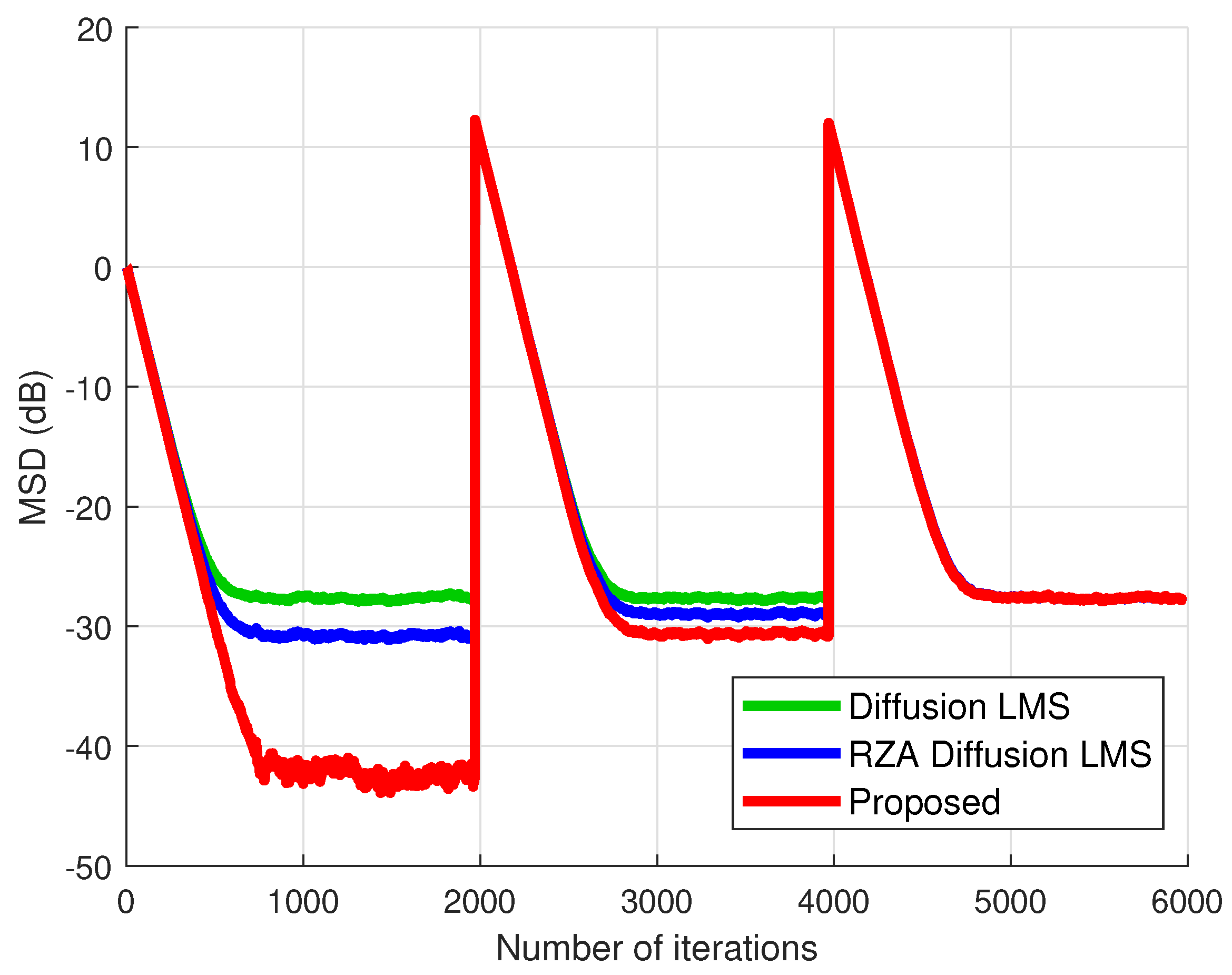
4.1. Performance Comparison

We conducted computer simulations to illustrate the effectiveness of our proposed algorithm.

Example of simulation setup: We consider a network topology composed of 16 interconnected nodes, as depicted in the top of Figure 1. The input regressors have zero-mean white Gaussian distribution with variances ${\sigma }_{u,k}^2$ as illustrated in the middle of Figure 1. The background white noise power of individual nodes, denoted by ${\sigma }_{v,k}^2$, are shown in the bottom of Figure 1. The combination matrix A employs relative-degree weights, which are defined as $a_{l,k}=\frac{n_l}{\left({\sum }_{m\in {\mathcal{N}}_k}{n}_m\right)}$. The adaptation matrix C uses the Metropolis weights described by $c_{l,k}=\frac{1}{\max (n_k,n_l)}$ [6,29]. Here, $n_k$ represents the degree of node k, which corresponds to the size of its neighboring nodes. The length of the unknown vector is set to $M=32$, and the regressor vector has the same size. Our study involves three unknown channels with 32 weights, reflecting various sparsity scenarios as shown in Figure 2. We designate only one from the 32 weights of $w^o$ as one, resulting in a highly sparse system. Following 2000 iterations, we activate 16 randomly selected weights with one, leading to a sparsity ratio of 50%. After 4000 iterations, all weights are set to one, giving us a fully dense (non-sparse) system.

Performance comparison: In Figure 3, we present the learning curves related to network MSD for three distinct diffusion algorithms: diffusion LMS [13], RZA diffusion LMS [30], and our proposed algorithm. To ensure a balanced comparison, we used a consistent step size of $\mu =0.03$ across all algorithms. We derived our simulation outcomes by averaging over 50 independent trials. The sparsity parameters of the RZA diffusion LMS were determined as $\gamma =5\times {10}^{-5}$ and $\epsilon =0.01$. Meanwhile, the parameters for our proposed algorithm were set to $\gamma =5\times {10}^{-5}$ and $\alpha =3.25$ (with $\rho \approx$ 1800) to ensure an identical rate of convergence across all algorithms. As shown in Figure 3, in a highly sparse system, our proposed algorithm consistently outperforms both the standard diffusion LMS and the conventional RZA diffusion LMS algorithms in terms of steady-state performance. Our steady-state error is approximately 11.6 dB and 14.7 dB lower than that of the RZA diffusion LMS and standard diffusion LMS algorithms, respectively. For systems where the unknown vector exhibits 50% sparsity, our proposed algorithm demonstrated the lowest error, which is 2.1 dB and 3.3 dB lower than the respective algorithms. While sparse diffusion LMS algorithms still maintain a lower steady-state MSD compared to the standard diffusion LMS, the performance difference becomes less pronounced as sparsity decreases. In fully dense systems, the performance of all algorithms appears largely equivalent.

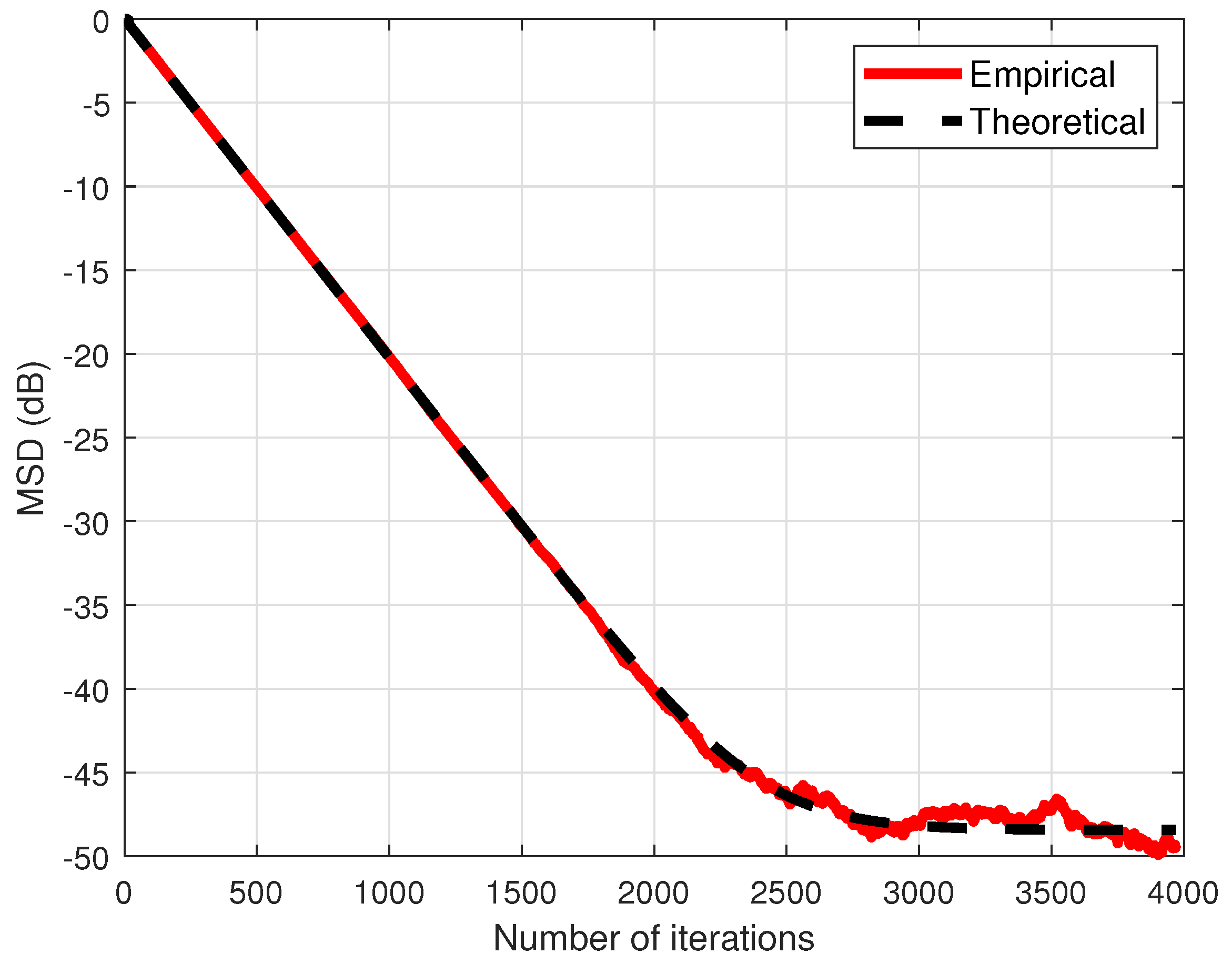
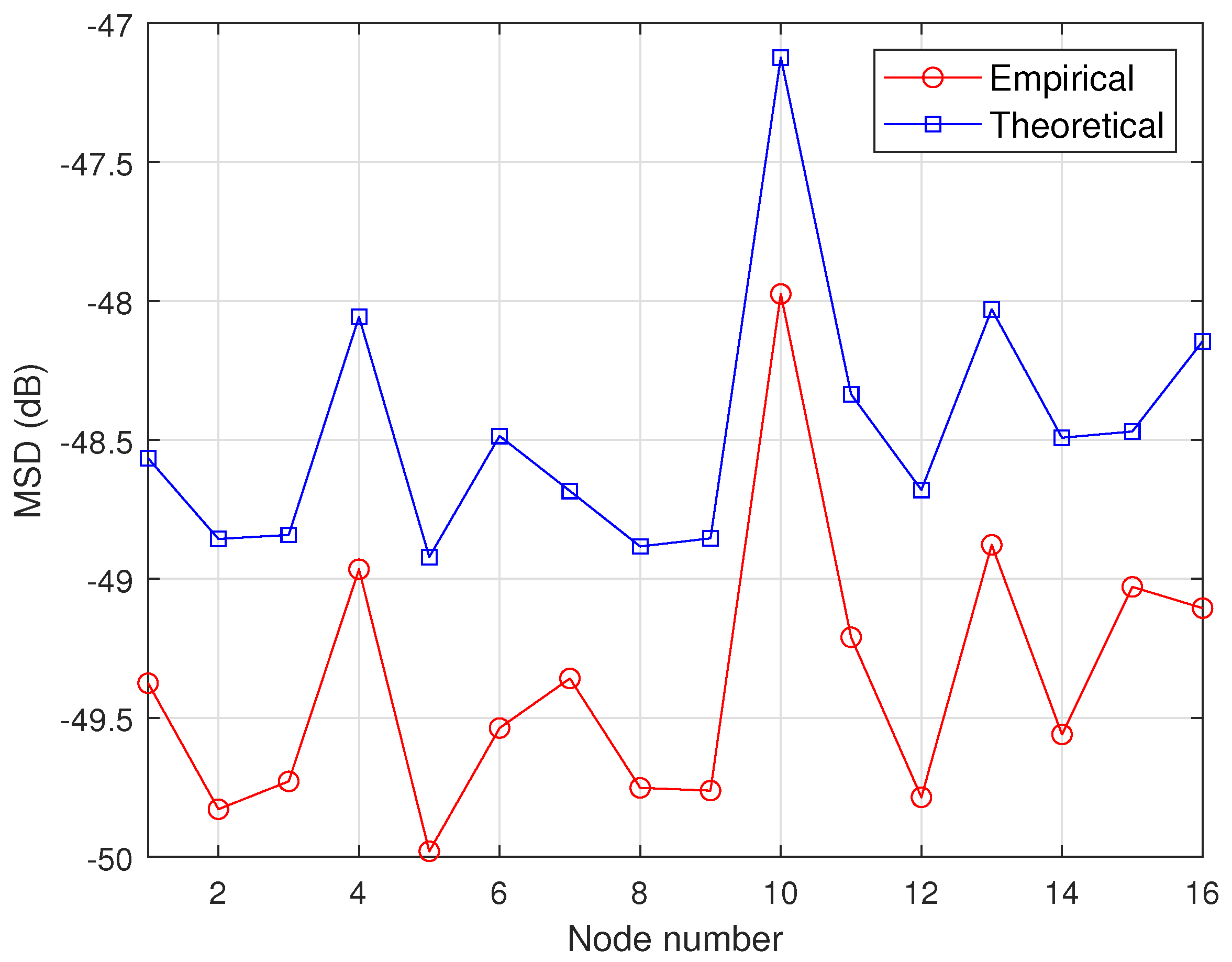
4.2. Theoretical Validation

In this subsection, we validate our theoretical findings compared to the empirical results. For this simulation, only the 9th weight was set to one and the others were set to zeros. The step size was set to $\mu =0.01$. The other parameters remained consistent with those outlined in Section 4.1.

Figure 4 displays the transient network MSD of our proposed algorithm alongside its theoretical result. The theoretical result is well matched with the empirical result throughout all iterations.

Finally, to verify the steady-state MSE analysis, the theoretical result (62) is compared with the simulation outcomes at each node as shown in Figure 5. Despite the theoretical results being slightly higher than the empirical results at the steady state, their overall agreement is satisfactory. This minor deviation can be attributed to the simplifications in our analysis stemming from several assumptions and approximations.

5. Conclusions

In this paper, we introduced a novel sparse distributed estimation method based on the diffusion LMS algorithm. Sparse systems are typically characterized by the predominance of zero coefficients. To achieve this sparse representation, we incorporated $L_0$-norm regularization into the diffusion LMS update equation and employed a hard-thresholding technique. Our rigorous statistical analysis resulted in theoretical insights into the mean stability as well as both transient and steady-state MSD behaviors. Simulation results confirmed the improvement of our proposed algorithm and exhibited the consistency between the theoretical results and empirical observations. Significantly, our proposed algorithm demonstrated superior performance compared to conventional sparse algorithms, including the standard diffusion LMS and RZA diffusion LMS, especially in the highly sparse system scenario of distributed estimation over networks. Based on our findings, we recognize the need to expand on the current limitations. Future work will explore enhancements to the sparse diffusion normalized LMS (NLMS) and sparse diffusion affine projection algorithms, aiming to speed up the convergence rate in the presence of highly correlated input signals.

References

1. Sayed, A.H. Adaptation, learning, and optimization over networks. Found. Trends Mach. Learn. 2014, 7, 311–801. [Google Scholar] [CrossRef]
2. Lopes, C.G.; Sayed, A.H. Incremental adaptive strategies over distributed networks. IEEE Trans. Signal Process. 2007, 55, 4064–4077. [Google Scholar] [CrossRef]
3. Schizas, I.D.; Mateos, G.; Giannakis, G.B. Distributed LMS for consensus-based in-network adaptive processing. IEEE Trans. Signal Process. 2009, 57, 2365–2382. [Google Scholar] [CrossRef]
4. Soatti, G.; Nicoli, M.; Savazzi, S.; Spagnolini, U. Consensus-based algorithms for distributed network-state estimation and localization. IEEE Trans. Signal Inf. Process. Netw. 2016, 3, 430–444. [Google Scholar] [CrossRef]
5. Lopes, C.G.; Sayed, A.H. Diffusion least-mean squares over adaptive networks: Formulation and performance analysis. IEEE Trans. Signal Process. 2008, 56, 3122–3136. [Google Scholar] [CrossRef]
6. Cattivelli, F.S.; Sayed, A.H. Diffusion LMS strategies for distributed estimation. IEEE Trans. Signal Process. 2010, 58, 1035–1048. [Google Scholar] [CrossRef]
7. Liu, Y.; Li, C.; Zhang, Z. Diffusion sparse least-mean squares over networks. IEEE Trans. Signal Process. 2012, 60, 4480–4485. [Google Scholar] [CrossRef]
8. Sayed, A.H. Diffusion adaptation over networks. In Academic Press Library Signal Processing; Elsevier: Amsterdam, The Netherlands, 2014; Volume 3, pp. 323–453. [Google Scholar]
9. Tu, S.Y.; Sayed, A.H. Diffusion strategies outperform consensus strategies for distributed estimation over adaptive networks. IEEE Trans. Signal Process. 2012, 60, 6217–6234. [Google Scholar] [CrossRef]
10. Lee, J.W.; Kim, S.E.; Song, W.J.; Sayed, A.H. Spatio-temporal diffusion strategies for estimation and detection over networks. IEEE Trans. Signal Process. 2012, 60, 4017–4034. [Google Scholar] [CrossRef]
11. Jung, S.M.; Seo, J.H.; Park, P. A variable step-size diffusion normalized least-mean-square algorithm with a combination method based on mean-square deviation. Circuits Syst. Signal Process. 2015, 34, 3291–3304. [Google Scholar] [CrossRef]
12. Yu, Y.; He, H.; Yang, T.; Wang, X.; de Lamare, R.C. Diffusion normalized least mean M-estimate algorithms: Design and performance analysis. IEEE Trans. Signal Process. 2020, 68, 2199–2214. [Google Scholar] [CrossRef]
13. Cattivelli, F.S.; Lopes, C.G.; Sayed, A.H. Diffusion recursive least-squares for distributed estimation over adaptive networks. IEEE Trans. Signal Process. 2008, 56, 1865–1877. [Google Scholar] [CrossRef]
14. Li, L.; Chambers, J.A. Distributed adaptive estimation based on the APA algorithm over diffusion networks with changing topology. In Proceedings of the IEEE Statistical Signal Processing Workshop, Cardiff, UK, 31 August–3 September 2009; pp. 757–760. [Google Scholar]
15. Takahashi, N.; Yamada, I.; Sayed, A.H. Diffusion least-mean squares with adaptive combiners: Formulation and performance Analysis. IEEE Trans. Signal Process. 2010, 58, 4795–4810. [Google Scholar] [CrossRef]
16. Lee, H.S.; Kim, S.E.; Lee, J.W.; Song, W.J. A variable step-size diffusion LMS algorithm for distributed estimation. IEEE Trans. Signal Process. 2015, 63, 1808–1820. [Google Scholar] [CrossRef]
17. Chu, Y.; Chan, S.C.; Zhou, Y.; Wu, M. A new diffusion variable spatial regularized LMS algorithm. Signal Process. 2021, 188, 108207. [Google Scholar] [CrossRef]
18. Shi, K.; Shi, P. Convergence analysis of sparse LMS algorithms with l1-norm penalty based on white input signal. Signal Process. 2010, 90, 3289–3293. [Google Scholar] [CrossRef]
19. Wagner, K.; Doroslovacki, M. Proportionate-type normalized least mean square algorithms with gain allocation motivated by mean-square error minimization for white input. IEEE Trans. Signal Process. 2011, 59, 2410–2415. [Google Scholar] [CrossRef]
20. Murakami, Y.; Yamagishi, M.; Yukawa, M.; Yamada, I. A sparse adaptive filtering using time-varying soft-thresholding techniques. In Proceedings of the IEEE International Conference on Acoustics, Speech and Signal Processing, Dallas, TX, USA, 14–19 March 2010; pp. 3734–3737. [Google Scholar]
21. Su, G.; Jin, J.; Gu, Y.; Wang, J. Performance analysis of l_0 norm constraint least mean square algorithm. IEEE Trans. Signal Process. 2012, 60, 2223–2235. [Google Scholar] [CrossRef]
22. Chen, Y.; Gu, Y.; Hero III, A.O. Sparse LMS for system identification. In Proceedings of the IEEE Internatinal Conference on Acoustics, Speech and Signal Processing, Taipei, Taiwan, 19–24 April 2009; pp. 3125–3128. [Google Scholar]
23. Lee, H.S.; Lee, J.W.; Song, W.J.; Kim, S.E. Adaptive algorithm for sparse system identification based on hard-thresholding techniques. IEEE Trans. Circuits Syst. II Exp. Briefs 2020, 67, 3597–3601. [Google Scholar] [CrossRef]
24. Donoho, D.L. Compressed sensing. IEEE Trans. Inf. Theory 2006, 52, 1289–1306. [Google Scholar] [CrossRef]
25. Yang, X.; Wu, L.; Zhang, H. A space-time spectral order sinc-collocation method for the fourth-order nonlocal heat model arising in viscoelasticity. Appl. Math. Comput. 2023, 457, 128192. [Google Scholar] [CrossRef]
26. Wang, W.; Zhang, H.; Jiang, X.; Yang, X. A high-order and efficient numerical technique for the nonlocal neutron diffusion equation representing neutron transport in a nuclear reactor. Ann. Nucl. Energy 2023, 195, 110163. [Google Scholar] [CrossRef]
27. Jiang, X.; Wang, J.; Wang, W.; Zhang, H. A predictor-corrector compact difference scheme for a nonlinear fractional differential equation. Fractal Fract. 2023, 7, 521. [Google Scholar] [CrossRef]
28. Yim, S.H.; Lee, H.S.; Song, W.J. Proportionate diffusion LMS algorithm for sparse distributed estimation. IEEE Trans. Circuits Syst. II Exp. Briefs 2015, 62, 992–996. [Google Scholar] [CrossRef]
29. Lee, H.S.; Yim, S.H.; Song, W.J. z2-proportionate diffusion LMS algorithm with mean square performance analysis. Signal Process. 2017, 131, 154–160. [Google Scholar] [CrossRef]
30. Lorenzo, P.D.; Sayed, A.H. Sparse distributed learning based on diffusion adaptation. IEEE Trans. Signal Process. 2013, 61, 1419–1433. [Google Scholar] [CrossRef]
31. Das, B.K.; Chakraborty, M.; Arenas-García, J. Sparse distributed estimation via heterogeneous diffusion adaptive networks. IEEE Trans. Circuits Syst. II Exp. Briefs 2016, 63, 1079–1083. [Google Scholar] [CrossRef]
32. Kumar, K.S.; George, N.V. Polynomial sparse adaptive estimation in distributed networks. IEEE Trans. Circuits Syst. II Exp. Briefs 2018, 65, 401–405. [Google Scholar]
33. Nautiyal, M.; Bhattacharjee, S.S.; George, N.V. Robust and sparse aware diffusion adaptive algorithms for distributed estimation. IEEE Trans. Circuits Syst. II Exp. Briefs 2022, 69, 239–243. [Google Scholar] [CrossRef]
34. Huang, W.; Chen, C.; Yao, X.; Li, Q. Diffusion fused sparse LMS algorithm over networks. Signal Process. 2020, 171, 107497. [Google Scholar] [CrossRef]
35. Huang, W.; Shan, H.; Xu, J.; Yao, X. Adaptive diffusion pairwise fused Lasso LMS algorithm over networks. IEEE Trans. Neural Netw. Learn. Syst. 2023, 34, 5816–5827. [Google Scholar] [CrossRef] [PubMed]
36. Martin, R.K.; Sethares, W.A.; Williamson, R.C.; Johnson, C.R. Exploiting sparsity in adaptive filters. IEEE Trans. Signal Process. 2002, 50, 1883–1894. [Google Scholar] [CrossRef]
37. Krishnan, D.; Fergus, R. Fast image deconvolution using hyper-Laplacian priors. In Proceedings of the Advances in Neural Information Processing Systems, Vancouver, BC, Canada, 6–11 December 2009; pp. 1033–1041. [Google Scholar]
38. Zuo, W.; Meng, D.; Zhang, L.; Feng, X.; Zhang, D. A generalized iterated shrinkage algorithm for non-convex sparse coding. In Proceedings of the IEEE International Conference on Computer Vision, Sydney, Australia, 1–8 December 2013; pp. 217–224. [Google Scholar]
39. Haykin, S.S. Adaptive Filter Theory; Pearson Education India: Noida, India, 2005. [Google Scholar]
40. Haddad, D.B.; Petraglia, R. Transient and steady-state MSE analysis of the IMPNLMS algorithm. Digital Signal Process. 2014, 33, 50–59. [Google Scholar] [CrossRef]
41. Saeed, M.O.B.; Zerguine, A.; Zunmo, S.A. A variable step-size strategy for distributed estimation over adaptive networks. EURASIP J. Adv. Signal Process. 2013, 1, 135. [Google Scholar] [CrossRef]
Figure 1. Network topology with 16 interconnected nodes (top), regressor variances σ u , k 2 (middle), and noise variances σ v , k 2 (bottom).
Mathematics 11 04638 g001
Figure 2. Unknwon vectors: Channel 1 (top), Channel 2 (middle), and Channel 3 (bottom).
Mathematics 11 04638 g002
Figure 3. Network MSD comparison of the proposed algorithm with the standard [13] and RZA [30] diffusion LMS algorithms.
Mathematics 11 04638 g003
Figure 4. Theoretical transient MSD compared with empirical results.
Mathematics 11 04638 g004
Figure 5. Theoretical steady-state MSD at each node compared with empirical results.
Mathematics 11 04638 g005