A Group MCP Approach for Structure Identification in Non-Parametric Accelerated Failure Time Additive Regression Model

Abstract

In biomedical research, identifying genes associated with diseases is of paramount importance. However, only a small fraction of genes are related to specific diseases among the multitude of genes. Therefore, gene selection and estimation are necessary, and the accelerated failure time model is often used to address such issues. Hence, this article presents a method for structural identification and parameter estimation based on a non-parametric additive accelerated failure time model for censored data. Regularized estimation and variable selection are achieved using the Group MCP penalty method. The non-parametric component of the model is approximated using B-spline basis functions, and a group coordinate descent algorithm is employed for model solving. This approach effectively identifies both linear and nonlinear factors in the model. The Group MCP penalty estimation exhibits consistency and oracle properties under regularization conditions, meaning that the selected variable set tends to have a probability of approaching 1 and asymptotically includes the actual predictive factors. Numerical simulations and a lung cancer data analysis demonstrate that the Group MCP method outperforms the Group Lasso method in terms of predictive performance, with the proposed algorithm showing faster convergence rates.

1. Introduction

In both economic and biological research, it is a common scenario that many theories do not prescribe specific functional forms for the relationships between predictors and outcomes. For example, in biomedical studies, the influence of predictors on survival time can exhibit nonlinearity. Attempting to fit a linear model in such cases can result in biased estimates or produce misleading results. However, the functional shape of a non-parametric model is determined by the available data, eliminating the need for a linear functional form to describe the influence of a covariate. Additionally, non-parametric models offer greater flexibility in fitting data compared to parametric models. This paper delves into the in-depth study of the non-parametric accelerated failure time additive regression (NP-AFT-AR) model:

$$t_i=u+{\displaystyle \sum }_{j\in S_1}{\beta }_j{x}_{ij}+{\displaystyle \sum }_{j\in S_2}{f}_j\left(x_{ij}\right)+{\epsilon }_i i=1,2,\dots ,n$$

(1)

where ($t_i,x_{i1},\dots ,x_{ip}, 1\le i\le n$) is random sample, $t_i$ is the logarithm of the response variable, that is, $t_i$ is the logarithm of survival time. $x_{i1},\dots ,x_{ip}$ is a $p\times 1$ vector of covariates, $S_1,S_2$ are mutually independent and complementary subsets of $\left\{1,\dots ,p\right\}$, $\left\{{\beta }_j:jϵS_1\right\}$ are regression coefficients of the covariates with indices in $S_1$, and $\left\{f_j:jϵS_2\right\}$ are unknown functions. The covariates in $S_1$ have a linear relationship with the mean response, whereas the connection with the other covariates is not determined by a finite number of parameters. Parameter models require explicit assumption constraints, and they tend to overfit when there is an excessive number of model parameters. Some of these models are also based on the assumption of linearity, making them inadequate for capturing complex nonlinear relationships. However, parameter models offer the advantages of clear interpretability for explicit parameters, efficiency, and accurate parameter estimation. Hence, this paper aims to leverage these characteristics of parameter models and explores a hybrid approach that combines both parameter and non-parameter models to enhance the adaptability and performance of the model. When the emphasis is on the relationship between $t_i$ and $\left\{x_{ij}:jϵS_1\right\}$, which can be approximated by a linear function. It provides enhanced interpretability compared to a purely non-parametric additive model. The random error term ${\epsilon }_i$ has a mean of zero and a finite variance ${\sigma }^2$. Assuming that certain components $f_j$ are zero, our main objective in this research is to distinguish the nonzero components from the zero components and estimate the nonzero components accurately. A secondary objective is to elucidate the functional forms of the nonzero components, thereby suggesting a more concise model. The techniques we have established can readily be expanded to the partly linear additive AFT regression model, particularly when certain covariates may be discrete and not amenable to modeling using smoothing techniques like B-splines. We utilize the lung cancer data example to demonstrate this extension.

The structure identification method is effective in distinguishing linear variables from nonlinear ones, and numerous scholars have contributed to relevant research methods. Tibshirani [1] combined the least square estimation technique introduced by Bireman [2] with minimizing the residual sum of squares under constraints, transforming the solution into a continuous optimization process. This approach is known as the Lasso method, where penalties are applied to select variables, and estimated coefficients are continuously shrunk toward zero to automatically identify important explanatory variables. However, researchers such as Zhao and Yu [3] and Zou [4] discovered that the Lasso method may not consistently select the correct model, and the estimated regression coefficients do not exhibit asymptotic normality. To address this limitation, Fan and Li [5] proposed the SCAD penalty, which substitutes the penalty in Lasso with a quadratic spline penalty function to reduce deviations. In the context of linear models, the SCAD method can uniformly identify the true model and possess oracle properties. Nonetheless, the non-convex nature of the SCAD penalty makes it challenging to optimize in practical applications, leading to numerical instability during the solution process. Zhang [6] introduced the non-concave MCP (smoothly clipped absolute deviation) penalty and developed the MCP penalty likelihood procedure as an alternative approach. The MCP penalty method replaces the ${\mathcal{l}}_1$ penalty in Lasso with a quadratic spline penalty function to reduce bias. MCP exhibits the capability to consistently select the correct model with a probability of 1 and provides corresponding estimates with oracle properties.

Heller [7] employed the weighted kernel smooth rank regression method to estimate the unknown parameters in the AFT model, particularly in the case of censored data. Gu [8] introduced an empirical model selection approach for non-parametric components based on the Kullback–Leibler geometric structure. Schumaker [9] utilized the Lasso iterative method for selecting parametric covariates, while non-parametric components were estimated using the sieve method. Johnson [10] extended the rank-based Lasso-type estimation, which can encompass a portion of the linear AFT model. Huang and Ma [11] applied the AFT model to analyze the relationship between gene expression and survival time, using the bridge penalty method for individual-level regularized estimation and gene selection. Long et al. [12] established a risk prediction score through regularized rank estimation within a portion of the linear AFT model. Wei et al. [13] explored the application extension of subgroup identification methods based on Adaptive Elastic Net and the AFT model. Wang and Gao [14] conducted empirical likelihood inference for the AFT model under right-censored data. Cai et al. [15] compared parametric and semiparametric AFT models in clustered survival data. Liu et al. [16] introduced a new semiparametric approach that allows for the simultaneous selection of important variables, model structure identification, and covariate effect estimation within the AFT model.

Researchers used different methods for variable selection and parameter estimation. For instance, Fan and Li [5] employed the Newton algorithm to estimate the penalty likelihood function. Cui et al. [17] introduced the concept of penalty regression spline approximation and group structure identification within the additive model. However, their approach faced computational instability issues as they relied on truncated power series to approximate non-parametric truncation. Huang and Ma [11] proposed a two-step method where, with a fixed number of predictors, nonzero variables are simultaneously selected and estimated in the additive model, using Group Lasso in the first stage and Adaptive Group Lasso in the second stage. Leng and Ma [18] used the COSSO penalty to handle non-parametric covariate effects in the AFT model. However, due to the non-smooth nature of the penalty function at the origin, the computation can be challenging, and these methods require a significant amount of time to calculate the inverse matrix of the Hessian matrix, especially when dealing with high-dimensional covariates. Therefore, in this paper, the group coordinate descent (GCD) algorithm is employed to approximate and estimate the parameters in the non-parametric additive accelerated failure time model. GCD capitalizes on the assumption of model sparsity, and the algorithm is simple and operates at a fast pace. The GCD algorithm closely resembles the standard Newton–Raphson algorithm, but each iteration involves solving a weighted least squares problem with a penalty function.

Under the assumption that the dimensionality of covariates is allowed to diverge, this paper rigorously proves that the Group MCP penalty estimator in the non-parametric accelerated failure time model exhibits consistency and oracle properties. As the generalized cross-validation criterion is inconsistent in model selection when the sample size tends to infinity, meaning it may select irrelevant variables, the Bayesian Information Criterion (BIC) does not suffer from such issues. BIC, as shown by Golub et al. [19], has the desirable property of selecting the true model with a probability of 1. Therefore, in the context of structure identification in the non-parametric accelerated failure time model, this study opts for tuning based on the BIC criterion.

The remaining sections of the paper are organized as follows. In Section 2, we describe the construction of the AFT model with penalty estimation and variable selection based on Group MCP. Section 3 introduces the algorithm and parameter tuning for the effective identification of both linear and nonlinear factors in the model. In Section 4, we provide proof of the Group MCP’s selection consistency property, where the selected variable set asymptotically tends to include the actual predictive factors with a probability approaching 1. 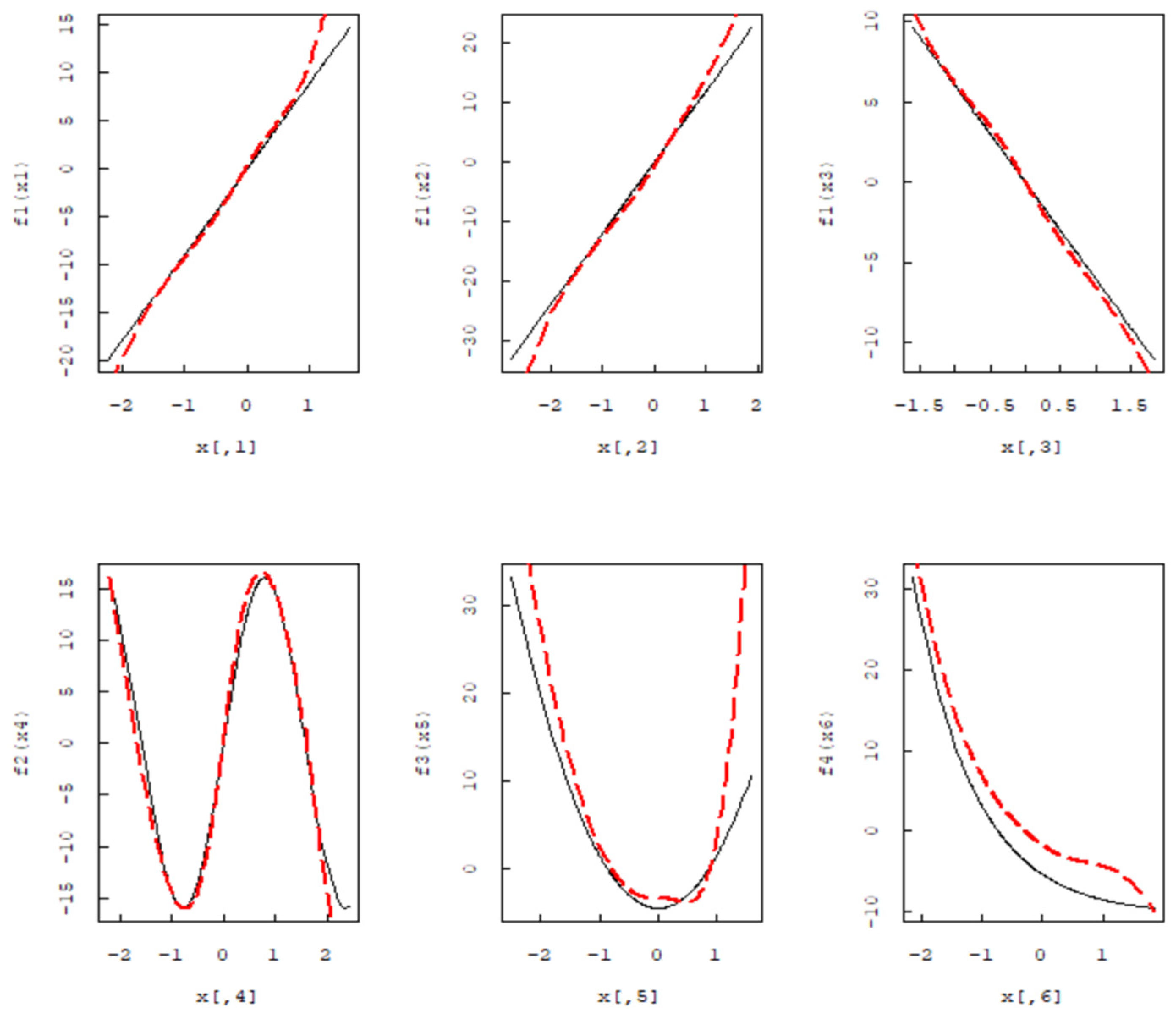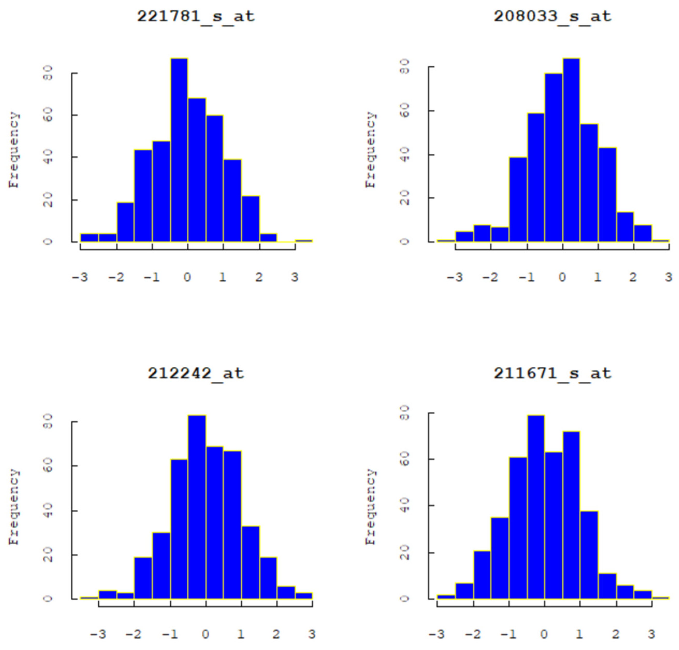Section 5 primarily focuses on numerical simulations and empirical analysis, demonstrating the method’s strong predictive performance. We also apply the method to the analysis of lung cancer data. Section 6 provides a brief summary of the corresponding conclusions.

2. Penalized Estimation and Variable Selection

2.1. Method

$T_i$ is the natural logarithm of the $i^{th}$ censoring time, $C_i$ is the natural logarithm of the survival time and ${\delta }_i$ represents the event indicator, i.e., ${\delta }_i=I\left(T_i\le C_i\right)$, which takes value 1 if the event time is observed or 0 if the event time is censored. $Y_i$ is the logarithm of the minimum of the survival time and the censoring time, i.e., $Y_i=\mathit{log}\left[\mathit{min}\left(T_i,C_i\right)\right]$. Then, the observed data are assumed to be independent and identically distributed (i.i.d.) samples from $\left(Y,\delta ,X\right)$, in the form of $\left(X_i,{\delta }_i,Y_i\right), i=1,\cdots ,n$. $Y_{\left(1\right)}\le Y_{\left(2\right)}\le \cdots \le Y_{\left(n\right)}$ is the order statistics of $Y_i{}^{\prime }\mathrm{s}$, ${\delta }_{\left(1\right)},\cdots ,{\delta }_{\left(n\right)}$, and $X_{\left(1\right)},\cdots ,X_{\left(n\right)}$ are the respective censoring indicators and covariates. F represents the distribution of T, and ${\widehat{F}}_n$ is its Kaplan–Meier estimator by [20].${\widehat{F}}_n\left(y\right)={\displaystyle \sum }_{i=1}^n{w}_{ni}I\left(Y_{\left(i\right)}\le y\right)$, where the $w_{ni}{}^{\prime }s$ are Kaplan–Meier weights calculated by $w_{n1}={\delta }_{\left(1\right)}/n$, and $w_{ni}=\left[{\delta }_{\left(i\right)}/(n-i+1\right)]{{\displaystyle \prod }}_{j=1}^{i-1}{\left(\left(n-j\right)/\left(n-j+1\right)\right)}^{{\delta }_{\left(j\right)}},i=2,\dots ,n$. After processing $T_i$ and considering whether $T_i\le C_i$ is established, transform $T_i$ into $Y_i$, when other conditions remain unchanged, the above conversion Formula (1) can be expressed as

$$Y_i=u+{\displaystyle \sum }_{j\in S_1}{\beta }_j{x}_{ij}+{\displaystyle \sum }_{j\in S_2}{f}_j\left(x_{ij}\right)+{\epsilon }_i i=1,2,\dots ,n$$

(2)

The following introduces the method of coefficient estimation in Equation (2), assuming that each group is orthonormal, i.e., $X_j^{\prime }{X}_k=0$, $j\ne k$ and $X_j^{\prime }{X}_j/n=I_{d_j}$. $\mathrm{z}=X_j^{\prime }\mathrm{y}/n$ is the least squares estimate of $\theta$, where $\theta$ is the unknown parameter associated with marker effects by [21]. Because of $X_j^{\prime }{X}_j/n=I_{d_j}$, the least squares objective function with penalty term can be expressed as $2^{-1}\parallel z-\theta {\parallel }_2^2+\rho \left(\parallel \theta {\parallel }_2;\lambda ,\gamma \right)$. The linear part of Formula (2) is expressed as a function and then is brought into the additive non-parametric regression model to obtain:

$$y_i=u+f_1\left(x_{i1}\right)+\cdots +f_p\left(x_{ip}\right)+{\epsilon }_{i }$$

(3)

To ensure unique identification of the $f_j{}^{\prime }\mathrm{s}$, we assume that $E{f}_j\left(x_{ij}\right)=0,1\le j\le p$. If some of the $f_j{}^{\prime }\mathrm{s}$ are linear, then Equation (3) transforms into the partially linear additive model (2). The problem shifts to determining the linear or nonlinear forms. Therefore, we decompose $f_j$ into a linear part and a non-parametric part $f_j\left(x\right)={\beta }_{0j}+{\beta }_{j}x+g_j\left(x\right)$. Consider a truncated series expansion for approximating $g_j$, that is $g_{nj}={\displaystyle \sum }_{k=1}^{m_n}{\theta }_{jk}{\phi }_k\left(x\right)$. Where $\left\{{\phi }_k\left(x\right),k=1,\dots ,m_n\right\}$ is a set of basis functions and $m_n\to \infty$ at certain rate as $n\to \infty$. If ${\theta }_{jk}=0, \left(1\le k\le m_n, j=1,\dots ,p\right)$, then $f_j$ has the linear form. Therefore, based on this equation, the current task is to ascertain which groups of $\left\{{\theta }_{jk},j=1,\dots ,p, k=1,\dots ,m_n\right\}$ are zero. Let $\beta ={\left({\beta }_1,\dots ,{\beta }_p\right)}^{\prime }$ and ${\theta }_n={\left({\theta }_{1n}{}^{\prime },\dots ,{\theta }_{pn}{}^{\prime }\right)}^{\prime }$, where ${\theta }_{jn}={\left({\theta }_{j1},\dots ,{\theta }_{j{m}_n}\right)}^{\prime }$. Define the penalized least squares criterion.

$$\begin{array}{cc}\hfill L\left(u,\beta ,\theta ;\lambda ,\gamma \right)=& \frac{1}{2n}{\displaystyle {\displaystyle \sum }_{i=1}^n}{w}_{ni}\Vert y_i-u-{\displaystyle {\displaystyle \sum }_{j=1}^p}{\beta }_j{x}_{ij}-{\displaystyle {\displaystyle \sum }_{j=1}^p}{\displaystyle {\displaystyle \sum }_{k=1}^{m_n}}{\theta }_{jk}{\phi }_k\left(x_{ij}\right){\Vert }_2^2\hfill \\ & +{\displaystyle {\displaystyle \sum }_{j=1}^p}{\rho }_{\gamma }(\Vert {\theta }_{jn}{\Vert }_{A_j};\sqrt{m_n}\lambda ) \hfill \end{array}$$

(4)

where $\rho$ is the penalty function based on the penalty parameter $\lambda \ge 0$ and regularization parameter $\gamma$. $u$ represents the intercept. $\Vert {\theta }_{nj}{\Vert }_{A_j}={\left({\theta }_{nj}{}^{\prime }{A}_j{\theta }_{nj}\right)}^{\frac{1}{2}}$ is the norm with respect to the positive definite matrix $A_j$. However, it is important to choose a suitable choice of $A_j$ to facilitate the computation. Let ${\tilde{X}}_{\left(i\right)}={\left(n{w}_{ni}\right)}^{1/2}\left(X_{\left(i\right)}-{\overline{X}}_W\right),$and ${\tilde{Y}}_{\left(i\right)}={\left(n{w}_{ni}\right)}^{1/2}\left(Y_{\left(i\right)}-{\overline{Y}}_W\right)$; ${\overline{X}}_W={\displaystyle \sum }_{i=1}^n{w}_{ni}{\mathit{X}}_{\left(i\right)}/{\displaystyle \sum }_{i=1}^n{w}_{ni}$ and ${\overline{Y}}_W={\displaystyle \sum }_{i=1}^n{w}_{ni}{Y}_{\left(i\right)}/{\displaystyle \sum }_{i=1}^n{w}_{ni}$, then the weight $w_{ni}$ in Formula (4) can not be expressed, and Formula (4) can be transformed into

$$L\left(\beta ,\theta ;\lambda ,\gamma \right)=\frac{1}{2n}{\displaystyle {\displaystyle \sum }_{i=1}^n}\Vert {\tilde{y}}_i-{\displaystyle {\displaystyle \sum }_{j=1}^p}{\beta }_j{\tilde{x}}_{ij}-{\displaystyle \sum }_{j=1}^p{\displaystyle \sum }_{k=1}^{m_n}{\theta }_{jk}{\phi }_k\left({\tilde{x}}_i\right){\Vert }_2^2+{\displaystyle \sum }_{j=1}^p{\rho }_{\gamma }(\Vert {\theta }_j{\Vert }_{A_j};\sqrt{m_n}\lambda )$$

(5)

We apply Group MCP penalty to the penalty term, i.e., ${\rho }_{\gamma }\left(t;\lambda \right)=\lambda {{\displaystyle \int }}_0^t{\left(1-x/\left(\gamma \lambda \right)\right)}_{+}dx,t\ge 0.$

$\gamma$ controls the concavity of $\rho$ and $\lambda$ is the penalty parameter. Here, $x_{+}$ denotes the nonnegative part of x, that is, $x_{+}=x{I}_{\left\{x\ge 0\right\}}$. We require $\lambda \ge 0 \mathrm{and} \gamma >1$. Taking the derivative with respect to ${\rho }_{\gamma }\left(t;\lambda \right)$ yields${\dot{\rho }}_{\gamma }\left(t;\lambda \right)=\lambda {\left(1-t/\left(\gamma \lambda \right)\right)}_{+},t\ge 0$. It initiates with the application of group MCP penalization at the same rate as the group lasso, gradually easing this penalization until, when $t>\lambda \gamma$, the rate of group MCP penalization diminishes to 0. This approach offers a spectrum of penalties, encompassing the ${\mathcal{l}}_1$ penalty at $\gamma =\infty$ and the hard-thresholding penalty when $\gamma \to 1+$. Notably, it encompasses the Lasso penalty as a specific case when $\gamma =\infty$.

The penalty in Equation (4) combines the penalty function ${\rho }_{\gamma }\left(·;\lambda \right)$ with a weighted ${\mathcal{l}}_2$ norm of ${\theta }_j$. ${\rho }_{\gamma }\left(·;\lambda \right)$ serves as a penalty for individual variable selection, and when applied to the norm of ${\theta }_j$, it selects the coefficients in ${\theta }_j$ as a group. This approach is favorable since the nonlinear components are captured by the coefficients in ${\theta }_j{}^{\prime }s$ as groups. We term the penalty function in Equation (4) as the group minimax concave penalty or simply the group MCP. The penalized least squares estimator is defined by $\left({\widehat{u}}_n,{\widehat{\beta }}_n,{\widehat{\theta }}_n\right)=\underset{u,\beta ,{\theta }_n}{argmin}L\left(u,\beta ,{\theta }_n;\lambda ,\gamma \right)$, subject to the constraints${\displaystyle \sum }_{i=1}^n{\displaystyle \sum }_{k=1}^{m_n}{\theta }_{jk}{\phi }_k\left(x_{ij}\right)=0, 1\le j\le p$. These centering constraints are sample analogs of the identifying restriction $E{f}_j\left(x_{ij}\right)=0,1\le i\le n,1\le j\le p$. $z_{ij}={\left({\phi }_{j1}\left(x_{ij}\right),\dots ,{\phi }_{j{m}_n}\left(x_{ij}\right)\right)}^{\prime }$, $z_{ij}$ consists of the centered basis functions at the $i$th observation of the $j$th covariate. Let $Z=\left(Z_1,\dots ,Z_P\right)$, where $Z_j={\left(z_{1j},\dots ,z_{nj}\right)}^{\prime }$ is the $n\times m_n$ design matrix corresponding to the $j$th expansion. Let $\tilde{\mathrm{y}}={\left({\tilde{y}}_1,\dots ,{\tilde{y}}_n\right)}^{\prime },{\tilde{x}}_i=\left({\tilde{x}}_{i1},\dots ,{\tilde{x}}_{ip}\right),$ and $\tilde{X}=\left({\tilde{x}}_1,\dots ,{\tilde{x}}_p\right)$. We can write

$$\left({\widehat{\beta }}_n,{\widehat{\theta }}_n\right)=\underset{\beta ,{\theta }_n}{argmin}\left\{L\left(\beta ,{\theta }_n;\lambda ,\gamma \right)=(1/2n)\Vert \tilde{y}-\tilde{X}\beta -Z{\theta }_n{\Vert }_2^2+{\displaystyle {\displaystyle \sum }_{j=1}^p}{\rho }_{\gamma }(\Vert {\theta }_{nj}{\Vert }_{A_j};\sqrt{m_n}\lambda )\right\}$$

(6)

Here, we excluded $u$ from the arguments of $L$, as the intercept is zero as a result of centering. Therefore, the constrained optimization problem transforms into an unconstrained one.

2.2. Penalized Profile Least Squares

The penalized profile least squares approach is used to calculate $\left({\widehat{\beta }}_n,{\widehat{\theta }}_n\right)$. The $\widehat{\beta }$ that minimizes $L$ inherently satisfies ${\tilde{X}}^{\prime }\left(\tilde{y}-\tilde{X}\beta -Z{\theta }_n\right)=0$ for any given ${\theta }_n$, resulting in $\beta ={({\tilde{X}}^{\prime }\tilde{X})}^{-1}{\tilde{X}}^{\prime }\left(\tilde{y}-Z{\theta }_n\right)$. Define $Q=I-P_{\tilde{X}}$, $P_{\tilde{X}}=\tilde{X}{({\tilde{X}}^{\prime }\tilde{X})}^{-1}{\tilde{X}}^{\prime }$ represents the projection matrix onto the column space of $\tilde{\mathrm{X}}$. Consequently, the profile objective function of ${\theta }_n$ becomes:

$$L\left({\theta }_n;\lambda ,\gamma \right)=(1/2n)\Vert Q\left(\tilde{y}-Z{\theta }_n\right){\Vert }^2+{\displaystyle {\displaystyle \sum }_{j=1}^p}{\rho }_{\gamma }(\Vert {\theta }_{nj}{\Vert }_{A_j};\sqrt{m_n}\lambda )$$

(7)

We use $A_j=n^{-1}{Z}_j^{\prime }{Q}^{\prime }{Z}_j$, this choice of $A_j$ standardizes the covariate matrices associated with ${\theta }_{nj}{}^{\prime }s$ and leads to an explicit expression for computation in the group coordinate algorithm described below. For any given $\left(\lambda ,\gamma \right)$, the penalized profile least squares estimator of ${\theta }_n$ is defined by ${\widehat{\theta }}_n=argmi{n}_{{\theta }_n}L\left({\theta }_n;\lambda ,\gamma \right)$. We compute ${\widehat{\theta }}_n$ using the group coordinate descent algorithm. The set of covariates estimated to have a linear form in the regression model (1) is denoted as ${\widehat{S}}_1\equiv \left\{j:\Vert {\widehat{\theta }}_{nj}\Vert =0\right\}$. Then, we obtain ${\widehat{g}}_{nj}\left(\tilde{x}\right)=0,j\in {\widehat{S}}_1 \mathrm{and} {\widehat{g}}_{nj}\left(\tilde{x}\right)={\displaystyle \sum }_{k=1}^{m_n}{\widehat{\theta }}_{jk}{\phi }_k\left(\tilde{x}\right),j\notin {\widehat{S}}_1$. Denote ${\widehat{X}}_{\left(1\right)}=\left(\left({\tilde{x}}_j\right), j\in {\widehat{S}}_1\right), {\widehat{Z}}_{\left(2\right)}=\left(Z_j:j\notin {\widehat{S}}_1\right)$ and ${\widehat{\theta }}_{n\left(2\right)}={\left({\widehat{\theta }}_{nj}^{\prime }:j\notin {\widehat{S}}_1\right)}^{\prime }$. We have ${\widehat{\beta }}_n={({\tilde{X}}^{\prime }\tilde{X})}^{-1}{\tilde{X}}^{\prime }\left(\tilde{y}-{\widehat{Z}}_{\left(2\right)}{\widehat{\theta }}_{n\left(2\right)}\right)$. Then, the estimator of the coefficients of the linear components is ${\widehat{\beta }}_{n1}={\left({\widehat{\beta }}_j: \mathrm{j}\in {\widehat{S}}_1\right)}^{\prime }, \widehat{g}\left(\tilde{\mathrm{x}}\right)={\left({\widehat{g}}_1\left(\tilde{\mathrm{x}}\right),\dots ,{\widehat{g}}_p\left(\tilde{\mathrm{x}}\right)\right)}^{\prime }$. Then, ${\widehat{\beta }}_{n1}={\left({\widehat{X}}_{\left(1\right)}^{\prime }{\widehat{X}}_{\left(1\right)}\right)}^{-1}{\widehat{X}}_{\left(1\right)}^{\prime }\left(y-{\displaystyle \sum }_{\mathrm{j}\notin {\widehat{S}}_1}{\widehat{g}}_j\left({\tilde{\mathrm{x}}}_i\right)\right)$ is the estimator of the coefficient vector of the linear components. The coefficients of the linear and nonlinear parts can be identified and estimated, and then the structure identification of the non-parametric can be added to the AFT model.

3. Computation

3.1. Computation Algorithm

Assuming that there is a standard between each group, i.e., $X_j^{\prime }{X}_k=0,j\ne k$ and $X_j^{\prime }{X}_j/n=I_{d_j}$. Let $z=X_j^{\prime }y/n$ is the least squares estimate of $\theta$. We use $S\left(z;t\right)={\left(1-t/\Vert z{\Vert }_2\right)}_{+}z$ to calculate the solution of group Lasso with the group coordinate descent algorithm, and the expression of group Lasso is ${\widehat{\theta }}_{\mathrm{gLASSO}}\left(\mathrm{z};\lambda \right)=S\left(\mathrm{z},\lambda \right)$. When $\gamma >1$, the group MCP of the quadratic norm can be expressed as ${\widehat{\theta }}_{\mathit{gMCP}}(\mathit{z}; \lambda ,\gamma )=\left\{\begin{array}{c}\frac{\gamma }{\gamma -1}S\left(z,\lambda \right) if \Vert z{\Vert }_2\le \gamma \lambda \\ z if \Vert z{\Vert }_2>\gamma \lambda \end{array}\right.$. When $\gamma \to \infty$, ${\widehat{\theta }}_{gMCP}\left(\cdot ;\lambda ,\gamma \right)\to {\widehat{\theta }}_{gLasso}\left(\cdot ;\lambda \right)$, for $\lambda >0$ and $\gamma \to 1$, ${\widehat{\theta }}_{gMCP}\left(\cdot ;\lambda ,\gamma \right)\to H\left(\cdot ;\lambda \right)$. $H\left(z;\lambda \right)\equiv \left\{\begin{array}{cc}0,& \mathit{if} \Vert z{\Vert }_2\le \lambda ,\\ z,& \mathit{if} \Vert z{\Vert }_2>\lambda .\end{array}\right.$. So we can use $\left\{{\widehat{\theta }}_{gMCP}\left(\cdot ;\lambda ,\gamma \right):1<\gamma \le \right.\infty \}$ to express hard threshold function of group MCP and when $\gamma =1$ or $\gamma =\infty$ can to be soft threshold function.

Group coordinate descent algorithm is used to compute ${\widehat{\theta }}_n$ in this paper. GCD algorithm is a natural extension of the standard coordinate descent algorithm [22,23] commonly used in optimization problems involving convex penalties like the Lasso. GCD algorithm optimizes the target function one group at a time, cycling through all groups iteratively until convergence is achieved. It is particularly well-suited for computing ${\widehat{\theta }}_n$ because it offers a straightforward closed-form expression for a single-group model, as presented in (8) below. $A_j=R_j^{\prime }{R}_j$ for an $m_n\times m_n$ upper triangular matrix $R_j$ via the Cholesky decomposition. Let $b_j=R_j{\theta }_j, \tilde{y}=Qy, {\tilde{Z}}_j=Q{Z}_j{R}_j^{-1}$. Simple algebra shows that $L\left(b;\lambda ,\gamma \right)=(1/2n)\Vert \tilde{y}-{\displaystyle \sum }_{j=1}^p{\tilde{Z}}_j{b}_j{\Vert }^2+{{\displaystyle \sum }}_{j=1}^p{\rho }_{\gamma }(\Vert b_j\Vert ;\sqrt{m_n}\lambda )$. Note that$n^{-1}{\tilde{Z}}_j{}^{\prime }{\tilde{Z}}_j=R_j^{-1}{}^{\prime }\left(n^{-1}{Z}_j^{\prime }Q{Z}_j\right)R_j^{-1}=I_{m_n}$. Let ${\tilde{y}}_j=\tilde{y}-{\displaystyle \sum }_{k\ne j}^p{\tilde{Z}}_k{b}_k$. Denote $L_j\left(b_j;\lambda ,\gamma \right)=(1/2n)\Vert {\tilde{y}}_j-{\tilde{Z}}_j{b}_j{\Vert }_2^2+{\rho }_{\gamma }\left(\Vert b_j\Vert ;\sqrt{m_n}\lambda \right)$. Let ${\eta }_j={\tilde{Z}}_j{({\tilde{Z}}_j{}^{\prime }{\tilde{Z}}_j)}^{-1}{\tilde{y}}_j=n^{-1}{\tilde{Z}}_j{}^{\prime }{\tilde{y}}_j$. when $\gamma >$ 1, the value minimizing $L_j$ with respect to $b_j$ is

$${\tilde{b}}_{j,GM}\left(\lambda ,\gamma \right)=M\left({\eta }_j;\lambda ,\gamma \right)=\left\{\begin{array}{cc}0, & if \Vert {\eta }_j\Vert \le \sqrt{m_n}\lambda \\ \frac{\gamma {\eta }_j}{\gamma -1}\left(1-\frac{\sqrt{m_n}\lambda }{\Vert {\eta }_j\Vert }\right), & if \sqrt{m_n}\lambda <\Vert {\eta }_j\Vert \le \gamma \sqrt{m_n}\lambda \\ {\eta }_j& if \Vert {\eta }_j\Vert >\sqrt{m_n}\lambda \end{array}\right.$$

(8)

In particular, when $\gamma =\infty$, we have ${\tilde{b}}_{j,GL}={\left(1-\sqrt{m_n}\lambda /\Vert {\eta }_j\Vert \right)}_{+}{\eta }_j$, which is the group Lasso estimate for a single-group model, GCD algorithm can be implemented as follows based on the above expressions. Let the group coefficient ${\tilde{b}}_k^{\left(s\right)},k\ne j$ is given. We want to minimize $L$ with respect to $b_j$. Define $L_j\left(b_j;\lambda ,\gamma \right)=(1/2n)\Vert \tilde{y}-{\displaystyle \sum }_{k\ne j}{\tilde{Z}}_k{\tilde{b}}_k^{\left(s\right)}-{\tilde{Z}}_j{\tilde{b}}_j^{\left(s\right)}{\Vert }^2+{\rho }_{\gamma }\left(\Vert b_j\Vert ;\sqrt{m_n}\lambda \right)$. Denote ${\tilde{y}}_j={{\displaystyle \sum }}_{k\ne j}{\tilde{Z}}_k{\tilde{b}}_k^{\left(s\right)}$ and ${\eta }_j=n^{-1}{\tilde{Z}}_j{}^{\prime }\left(\tilde{y}-{\tilde{y}}_j\right)$. Let ${\tilde{b}}_j$ denote the minimizer of $L_j\left(b_j;\sqrt{m_n}\lambda ,\gamma \right)$. When $\gamma >1$, we have ${\tilde{b}}_j=M\left({\eta }_j;\sqrt{m_n}\lambda ,\gamma \right)$. Equation (8) is used to iterate through one component at a time for any given $\left(\lambda ,\gamma \right)$. The initial value is ${\tilde{\beta }}^{\left(0\right)}={\left({\tilde{\beta }}_1^{{\left(0\right)}^{\prime }},\dots , {\tilde{\beta }}_p^{{\left(0\right)}^{\prime }}\right)}^{\prime }$. The proposed GCD algorithm is as follows: Initialize the residual vector $r=y-\tilde{y}$. Let $\tilde{y}={{\displaystyle \sum }}_{j=1,\dots ,p}{\tilde{Z}}_j{b}_j{}^{\left(0\right)}$. For $s=0,1,\dots ,$ carry out the following calculation until convergence. For $j=1,\dots ,p$, repeat the following steps:

(1)

Calculate ${\tilde{\eta }}_j=n^{-1}{\tilde{Z}}_j^{\prime }r+{\tilde{b}}_j^{\left(0\right)}.$

(2)

Update ${\tilde{b}}_j^{\left(s+1\right)}=M\left({\tilde{\eta }}_j;\lambda ,\gamma \right)$.

(3)

Update $r\leftarrow r-{\tilde{Z}}_j\left({\tilde{b}}_j^{\left(s+1\right)}-{\tilde{b}}_j^{\left(s\right)}\right)$ and $j\leftarrow j+1$.

The final step ensures that $r$ holds the current values of the residuals. While the objective function may not necessarily be convex, it exhibits convexity concerning an individual group when the coefficients of all other groups are fixed.

3.2. Tuning Parameter Selection

Methods such as AIC, BIC, and Generalized Cross-Validation (GCV) are widely used for selection consistency. Let $L\left(\cdot \right)$ be the likelihood function, and $\parallel \cdot {\parallel }_q$ represents the $L_q$ norm of the vector, $P_{\lambda }\left(\cdot \right)$ is a penalty function related to the parameter $\lambda >0$, The penalty method of structure recognition mainly considers the important variables by finding the extreme value of the objective function $(1/n)L\left(\beta \right)-{{\displaystyle \sum }}_{j=1}^p{P}_{\lambda }\left(\left|{\beta }_j\right|\right)$. Tibshirani [20] used the $L_1$ norm as the penalty function to obtain Lasso. AIC criterion is used to solve the over-fitting problem in which the value of the model likelihood function increases with the increase of the parameters, where $AIC=-2\mathit{log}\left(L\right)+2k$. BIC criterion penalizes the number of parameters more strongly, where $BIC=-2\mathit{log}\left(L\right)+kln\left(n\right)$. L is the maximum value of the likelihood function, k is the number of parameters in the model. When $\lambda$→0, $\beta$ close to ordinary least squares estimation; when $\lambda$→∞, almost only penalty items remain in the selection criteria. Therefore, we use the faster BIC method to select the parameters of each concave penalty model. The expression of the BIC criterion is $BIC\left(\lambda ,d_n\right)=\log \left(RS{S}_{\lambda ,d_n}\right)+lo{g}_n(d{f}_{\mathsf{\lambda },d_n})/n$. RSS is the sum of squared residuals, $df$ is the number of variables selected for a given ($\lambda$,$d_n$). $d_n$ is selected from an increasing sequence with multiple nodes, and then selects $\lambda$ from a sequence of length 100 for any given $d_n$. The maximum value of the sequence is ${\mathsf{\lambda }}_{max}=ma{x}_{1\le j\le p}\left(\Vert {\tilde{Z}}_j^{\prime }Y{\Vert }_2/\sqrt{d_n}\right)$, where $Z_j^{\prime }$ is a $n\times d_n$ dimensional matrix about the covariate $X_j, j=1,\dots ,p$, the minimum is $0.01{\lambda }_{max}$.

4. Theoretical Properties of Group MCP

Let $\left|A\right|$ denote the cardinality of any set $A\subseteq \left\{1,\dots ,p\right\}$, and $X_A=(X_j,j\in A,{\displaystyle \sum }_A=X_A^{\prime }W{X}_A/n$, where $X$ is $n\times p$ covariance matrix, $W=diag\left(n{w}_1,\dots ,n{w}_n\right)$. Let ${\beta }_0=\left\{{\beta }_{01},\dots ,{\beta }_{0p}\right\}$ be the true regression coefficient and $A_1=\left\{j:{\beta }_{0j}\ne 0\right\}$ be the set of nonzero regression coefficients, $q=\left|A_1\right|$ Represents the number of elements in the set $A_1$, and satisfies the following conditions:

(C1) $Eg\left(x_j\right)=0$ and there are constants $C_1$ and $C_2$such that the density distribution function ${\eta }_j\left(x\right)$ of$x_j$ satisfies $0<C_1\le {\eta }_j\left(x\right)\le C_2<\infty$ on [a,b] for $1\le j\le p$.

(C2) $\left(X_i,{\delta }_i,Y_i\right),i=1,\dots ,n$ is independent and identically distributed (i.i.d), and the error term ${\epsilon }_1,\dots ,{\epsilon }_i$ is i.i.d in $N\left(0,{\sigma }^2\right)$ and exists $K_1,K_2>0$, which is constant for all $x_i\ge 0$, $P\left(\left|{\epsilon }_i\right|>x_i\right)\le K_2\mathit{exp}\left(-K_1{x}_i^2\right)$.

(C3) The error term (${\epsilon }_1,\dots ,{\epsilon }_n$) is independent of the Kaplan–Meier weight ($w_1,\dots ,w_n$), and there is a constant satisfying that for any $1\le i\le n,1\le j\le p$, there is $\left|X_{ij}\right|\le M$, that is, the covariate is bounded.

(C4) The covariate matrix satisfies the SRC condition, exists $0<c_{*}<c^{*}<\infty ,q^{*}=\left(3+4C\right)q,C=C=c^{*}/c_{*}$, converges to 1 with probability and satisfies $c_{*}\le v^{\prime }{{\displaystyle \sum }}_{A}v/\Vert v{\Vert }^2\le c^{*}$.

Condition (C1) can ensure that the model is sparse even when the number of covariates is large; that is, the number of covariates with nonzero coefficients can be controlled to a small number; condition (C2) can ensure the tail probability of the model under high-dimensional linear regression The assumption is still valid; according to condition (C3), the sub-Gaussian nature of the model is still guaranteed even if the data is censored; (C4) Ensure that the model meets the SRC condition, that is, ensure that the characteristic root of matrix $X^{\prime }WX/n$ is always between $c_{*}$ and$c^{*}$, and any model with a dimension smaller than $q^{*}$ can be identified. Where $\tilde{\beta }=\left({\tilde{\beta }}_1,\dots ,{\tilde{\beta }}_p\right)$ represents the estimated coefficient, and $\widetilde{A_1}=\left\{j,{\tilde{\beta }}_j\ne 0\right\}$ represents a set of all nonzero coefficients. Denote $f_j\left(\mathrm{x}\right)={\beta }_{0j}+{\beta }_{j}x+g_j\left(x\right)$ is the regression component of the true value, $g_{nj}\left(x\right)={\displaystyle \sum }_{k=1}^{m_n}{\theta }_{jk}{\phi }_k\left(x\right),j=1,\dots ,p$ is B-spline basis function expansion of $g_{nj}\left(x\right)$, and $S_1=\left\{j:\Vert g_{nj}\left(x\right){\Vert }_2=0 \right\}$, $\Vert {\theta }_{nj}{\Vert }_2=0$. Let $q=\left|S_1\right|$ be the cardinality of $S_1$, which is the number of linear components in the AFT regression model. Define

$${\widehat{\theta }}_n=\underset{{\theta }_n}{argmin}\left\{\frac{1}{2n}\Vert Q\left(y-Z{\theta }_n\right){\Vert }^2:{\theta }_{nj}=0,jϵS_1\right\}$$

(9)

This represents the oracle estimator of ${\theta }_{0n}$ under the assumption that the identity of the linear components is known. It’s worth noting that the oracle estimator cannot be computed as $S_1$ is unknown. Nevertheless, we employ it as the reference point for evaluating our proposed estimator. Similar to the actual estimates outlined in Section 2.2, let’s define the oracle estimators as ${\tilde{g}}_{nj}\left(x\right)=0, jϵS_1 \mathrm{and} {\tilde{g}}_{nj}\left(x\right)={{\displaystyle \sum }}_{k=1}^{m_n}{\tilde{\theta }}_{jk}{\phi }_k\left(x\right), j\notin S_1$. Denote $X_{\left(1\right)}=\left(x_j, jϵS_1\right), X_{\left(2\right)}=\left(x_j, jϵS_2\right) \mathrm{and} {\tilde{\theta }}_{n\left(2\right)}={\left({\tilde{\theta }}^{\prime }{}_{nj}, jϵS_2\right)}^{\prime }$. Let ${\tilde{f}}_j\left(x\right)={\tilde{\beta }}_{0j}+{\tilde{\beta }}_{j}x+{\tilde{g}}_j\left(x\right),jϵS_2$.The oracle estimator of the coefficients of the linear components is ${\tilde{\beta }}_{n1}={(X^{\prime }{}_{\left(1\right)}{X}_{\left(1\right)})}^{-1}{X^{\prime }}_{\left(1\right)}\left(y-{{\displaystyle \sum }}_{jϵS_2}{\tilde{f}}_j\left(x\right)\right)$. Without loss of generality, suppose that $S_1=\left\{1,\dots ,q\right\}$. Write ${\tilde{\theta }}_n={\left(O_{q{m}_n}^{\prime },{\tilde{\theta }}^{\prime }{}_{\left(2\right)}\right)}^{\prime }$, where $O_{q{m}_n}$ is a $\left(q{m}_n\right)$-dimensional vector of zeros and${\tilde{\theta }}_{n\left(2\right)}={\left(Z_{\left(2\right)}^{\prime }Q{Z}_{\left(2\right)}\right)}^{-1}{Z}_{\left(2\right)}^{\prime }Qy$. ${\theta }_{*}=mi{n}_{jϵS_1}\Vert {\theta }_{0nj}\Vert$ represents the minimal coefficient norm in the B-spline expansions of the nonlinear components. Consider a non-negative integer $k$ and take $0<\alpha \le 1$, such that $d=k+\alpha >0.5$. Now, let’s define $\mathcal{G}$ as the set of functions $g$ on $\left[0,1\right]$, where the $\mathrm{kth}$ derivative $g^{\left(k\right)}$ exists and adheres to a Lipschitz condition of order $\alpha$: $\left|g^{\left(k\right)}\left(s\right)-g^{\left(k\right)}\left(t\right)\right|\le C{\left|s-t\right|}^{\alpha }$ for $s,tϵ\left[a,b\right]$.

Theorem 1.

Suppose that $m_n=O\left(n^{\frac{1}{2d+1}}\right)$, $\frac{1}{\sqrt{m_n\gamma }}$ is less than the smallest eigenvalue of $Z^{\prime }QZ/n$, and $\frac{1}{m_n^{\frac{2d-1}{2}}\left({\theta }_{*}-\lambda \gamma \right)}+\frac{1}{\lambda \sqrt{n}}\to 0$.

Then under (C1–C3), $P\left({\widehat{\theta }}_n\ne {\tilde{\theta }}_n\right)\to 0$, Consequently, $P\left(\widehat{S_1}=S_1\right)\to 1,P\left({\widehat{\beta }}_{n1}={\tilde{\beta }}_{n1}\right)\to 1$ and $P\left(\Vert {\widehat{f}}_{nj}\left(x\right)-{\tilde{f}}_{nj}\left(x\right){\Vert }_2=0,jϵS_2\right)\to 1$. Hence, given the conditions specified in Theorem 1, the proposed estimator can effectively differentiate between linear and nonlinear components with a high probability of accuracy. Additionally, the proposed estimator exhibits the oracle property, implying that it aligns with the oracle estimator’s performance, assuming the knowledge of linear and nonlinear component identities, except for events with vanishingly low probabilities.

Theorem 2.

Suppose (C1)–(C3) hold, we have

$${\displaystyle {\displaystyle \sum }_{j=1}^p}\Vert {\widehat{f}}_{nj}\left(x\right)-f_{0j}\left(x\right){\Vert }_2^2\le O_p\left(\frac{m_n}{n}\right)+O\left(\frac{1}{m_n^{2d}}\right)+O(m_n{\lambda }^2)$$

Theorem 2 provides the convergence rate of the proposed estimator within the non-parametric additive model, encompassing partially linear models as specific instances. Specifically, if we assume the second-order differentiability (d = 2) of each component and let $m_n=O\left(n^{\frac{1}{5}}\right)$ and $\lambda =n^{-\frac{1}{2}+\delta }$ tend toward small $\delta >0$, then ${{\displaystyle \sum }}_{j=1}^p\Vert {\widehat{f}}_{nj}\left(x\right)-f_{0j}\left(x\right){\Vert }_2^2=O_p\left(n^{-4/5}\right)$, representing the optimal convergence rate in non-parametric regression. We will now explore the asymptotic distribution of ${\widehat{\beta }}_{n1}$. Denote $H_j=\left\{h_j={\left(h_k:kϵS_1\right)}^{\prime }:E{h}_{jk}^2\left(u\right)<\infty \right\}, jϵS_2$. Each element of $H_j$ is a $\left|S_1\right|$-vector of square-integrable functions with mean zero. Let the sumspace $H=\left\{h={{\displaystyle \sum }}_{jϵS_2}{h}_j:h_jϵH_j\right\}$. The projection of the centered covariate vector $x_{\left(1\right)}-E\left(x_{\left(1\right)}\right)ϵR^q$ onto the sumspace $H$ is defined to be the ${\left(h_1^{*},\dots ,h_r^{*}\right)}^{\prime }$ with $E{h}_j^{*}\left(x_j\right)=0,j\le {\widehat{S}}_2$ that minimizes $W\left(h\right)=E\Vert x_{\left(1\right)}-E\left(x_{\left(1\right)}\right)-{{\displaystyle \sum }}_{j\in S_2}{h}_j\left(x_j\right){\Vert }^2$. For $x_{\left(2\right)}=\left(x_j:jϵS_2\right)$, denote $h^{*}\left(x_{\left(2\right)}\right)={{\displaystyle \sum }}_{j\in S_2}{h}^{*}{}_j\left(x_j\right)$. Therefore, the orthogonal projection $h^{*}$ onto $H$ is well-defined and unique. Additionally, each individual component $h^{*}{}_j$ is also well-defined and unique.

Theorem 3.

Assuming the conditions stated in Theorem 1 and the fulfillment of (C4), and given that A is non-singular. Then, $\sqrt{n}\left({\widehat{\beta }}_{n1}-{\beta }_{\left(1\right)}\right)\stackrel{d}{\to }N\left(0,\Sigma \right)$, where ${\beta }_{\left(1\right)}={\left({\beta }_j: jϵS_1\right)}^{\prime }$ and $\Sigma ={\sigma }^2{A}^{-1}$.

Theorem 3 provides sufficient conditions under which the proposed estimator ${\tilde{\beta }}_{n1}$ of the linear components in the model is asymptotically normal with the same limit normal distribution as the oracle estimator ${\tilde{\beta }}_{n1}$. Suppose that the first $q$ addable parts are important functions, and the remaining $p-q$ are non-important functions. Let $A_0=\left\{q+1,\cdots ,p\right\}$ be the set of non-important functions. Let $X=\left(X_1,\cdots ,X_p\right)$, $\mathsf{\Sigma }=X^{\prime }X/n$, for any $A\subseteq \left\{1,\cdots ,p\right\}$, $X_A=\left(X_j,j\in A\right)$, ${\mathsf{\Sigma }}_A=X_A^{\prime }{X}_A/n$, $\left|A\right|$ represents the cardinality of set A and $d_A=\left|A\right|d_n$.

5. Numerical Simulation and Empirical Analysis

5.1. Numerical Simulation

Simulation is employed to assess the performance of the group MCP method in finite samples. Two examples are included in the simulation. For each of these simulated models, we consider two sample sizes (n = 100, 200) and conduct a total of 100 replications. We examine the following four functions defined on $\left[0,1\right]$, $f_1\left(X_1\right)=\mathit{sin}\left(2X_1\right),f_2\left(X_2\right)=cos\left(X_2\right), f_3\left(X_3\right)=5X_3, \mathrm{and} f_4\left(X_4\right)=e^{-X_4}-2.5$. In the implementation, we utilize B-splines with seven basis functions to approximate each function.

Based on n = 200, the black solid line is the actual function, and the red dashed line is the Group MCP estimation function curve. It can be seen from Figure 1 that when the Group MCP method is used for B-spline expansion, the estimated function fits the real function well. In addition, we do not consider the intercept term of the model, $X_j, j=1,2,3,4,5,6 \mathrm{and} \epsilon$ independent and identically distributed in $N\left(0,0.1\right)$, some functions as follows:$f_1\left(X_1\right)=3X_1, f_2\left(X_2\right)=2\mathit{sin}\left(2X_2\right),f_3\left(X_3\right)=X_3^2-0.75, f_4\left(X_4\right)=e^{-X_4}-25/12$. Let q = 6. Consider the model $y=3f_1\left(x_1\right)+4f_1\left(x_2\right)-2f_1\left(x_3\right)+8f_2\left(x_4\right)+6f_3\left(x_5\right)+5f_4\left(x_6\right)+\epsilon$. In this model, the first three variables demonstrate a linear effect, while the last three variables exhibit a nonlinear effect. When n = 200, the black solid line is the actual function, and the red dashed line is the Group MCP estimation function curve. Figure 2 demonstrates that for the non-parametric additive accelerated failure time model, the non-parametric component estimates fit the true function well after B-spline estimation. In Figure 1 and Figure 2, the red dashed line represents the estimated function, while the black solid line represents the real function.

Table 1. The performance of group LASSO and group MCP.

Method	NL	ER	IN%	CS%	Time (min)
	p = 6 n = 100
group LASSO	1.25	0.31	100	100	2.51
	(1.14)	(0.16)	(0.00)	(0.00)
group MCP	2.35	0.24	100	100	1.23
	(1.01)	(0.15)	(0.00)	(0.00)
	p = 6 n = 200
group LASSO	0.26	0.15	100	100	4.49
	(0.51)	(0.05)	(0.00)	(0.00)
group MCP	0.69	0.13	100	100	3.47
	(0.67)	(0.04)	(0.00)	(0.00)
	p = 6 n = 500
group LASSO	0.19	0.11	100	100	7.36
	(0.24)	(0.01)	(0.00)	(0.00)
group MCP	0.36	0.08	100	100	6.18
	(0.27)	(0.01)	(0.00)	(0.00)

Note: the corresponding standard errors are in parentheses.

displays simulation results based on 1000 replications. The columns provide the following information: the average number of selected nonlinear components (NL), the average model error (ER), the percentage of occasions on which the correct nonlinear components are included in the selected model (IN%), and the percentage of occasions on which the exact nonlinear components are chosen (CS%) in the final model. To compare the computational efficiency of group Lasso and group MCP, using time units in minutes (Time). The standard errors corresponding to these values are enclosed in parentheses. The Group MCP penalty outperforms the Group Lasso in terms of both the percentage of occasions on which the correct nonlinear components are included in the selected model (IN%) and the percentage of occasions on which the exact nonlinear components are chosen (CS%) in the final model. As the sample size increases from 100 to 500, both methods exhibit improved performance in terms of including all the nonlinear components (IN%) and selecting the exact correct model (CS%). The computational efficiency of group MCP surpasses that of group Lasso. This improvement is expected as larger sample sizes provide more information about the underlying model.

Table 2. Mean square error of important functions.

Method	${\mathit{f}}_1\mathsf{(}.\mathsf{)}$	${\mathit{f}}_2\mathsf{(}.\mathsf{)}$	${\mathit{f}}_3\mathsf{(}.\mathsf{)}$	${\mathit{f}}_4\mathsf{(}.\mathsf{)}$	${\mathit{f}}_5\mathsf{(}.\mathsf{)}$	${\mathit{f}}_6\mathsf{(}.\mathsf{)}$
	n = 100
Group Lasso	24.44	52.29	20.00	79.21	18.44	67.58
Group MCP	22.88	45.17	17.79	69.88	20.80	111.05
	n = 200
Group Lasso	28.30	43.77	11.48	68.04	10.90	23.08
Group MCP	24.55	38.93	9.68	62.85	15.73	25.45
	n = 500
Group Lasso	30.40	23.78	8.17	32.34	4.92	6.13
Group MCP	27.62	16.82	5.46	26.15	2.37	8.54

shows the number of times each component is estimated as a nonlinear function. Table 2 shows that the Group MCP method is more accurate in distinguishing between linear and nonlinear functions compared to the Group Lasso. Additionally, the Group MCP penalty method results in smaller mean squared errors, indicating more accurate estimation. The research demonstrates that the proposed approach using the Group MCP penalty is effective in distinguishing between linear and nonlinear components in simulated models, thereby enhancing model selection and estimation accuracy.

5.2. Lung Cancer Data Example

This study is based on survival analysis using the survival time data of 442 lung cancer patients and the gene expression data of 22,283 genes extracted from tumor samples. These data are available from the official website of the National Cancer Institute (http://cancergenome.nih.gov/) (accessed on 12 November 2023). In the original data, a two-column matrix denoted as T represents the survival data. The first column contains survival time in months, while the second column serves as an indicator function where 1 represents the state of death, and 0 represents the state of survival. The measured gene expression data are represented as X, with 22,283 gene expressions. The objective of this study is to identify covariates with nonlinear effects on survival time.

Due to the high dimensionality of the original data (p = 22,283, n = 442), it is necessary to transform the data from high-dimensional to low-dimensional. Assuming that the correlation coefficient between the independent variable and the dependent variable is equal to 0, the alternative hypothesis posits that the correlation coefficient between the independent variable and the dependent variable is not equal to 0. R programming language program is used to calculate the p-value for the correlation coefficient between each gene expression and survival time. When the p-value is less than the critical value, the null hypothesis is rejected in favor of the alternative hypothesis, indicating a significant correlation between the independent variable and the dependent variable. A smaller p-value provides stronger evidence of the association between gene expression and survival time. In this study, the p-values of the independent variables are computed and sorted in ascending order, and the top 50 independent variables with the smallest p-values are selected as input variables. The remaining gene expressions are discarded, achieving initial dimensionality reduction. As a result, the original data are transformed into lower dimensional data (p = 50, n = 442), and then covariates with nonlinear effects on survival time are identified.

Figure 3 displays the frequency distribution histograms of four randomly selected gene expressions, indicating that the distributions of these four gene expressions are all skewed. Based on the skewed data, this study considered using a non-parametric additive AFT model, with B-spline basis functions used to expand each covariate in the non-parametric part. The Group MCP method was employed to select and compress the coefficients of the B-spline basis functions, ultimately identifying gene expressions with nonlinear effects on survival time. Furthermore,

Table 3. The genes selected by Group Lasso and Group MCP.

Gene Symbol	gLASSO	gMCP
208033_s_at	√
212242_at	√
211671_s_at	√
216364_s_at	√
205944_s_at	√
214143_x_at	√
217155_at	√
202734_at	√
219720_s_at	√	√
214991_s_at	√	√
214944_at	√
215544_s_at	√
217106_x_at	√
216180_s_at	√
208917_x_at	√
210802_s_at	√	√
221781_s_at	√
55583_at	√
204446_s_at	√

compares the results selected by the Group Lasso and Group MCP penalization methods. Under the Group Lasso penalization, all gene symbols were selected, indicating a tendency to over-select nonlinear variables. In contrast, Group MCP outperformed Group Lasso in selecting nonlinear variables. Genes 219720_s_at, 214991_s_at, and 210802_s_at were simultaneously selected, indicating that these three gene expressions are nonlinear variables. The three selected genes are associated with lung cancer research and can potentially be used to identify cancer biomarkers, understand tumor biology and develop treatment strategies. In order to comprehensively assess the significance of these specific genes in cancer research, further experimentation and literature studies are required. This decision may necessitate the support of specialized knowledge in the field of cancer biology and experimental data. This also represents a future direction for research.

The analysis compares the selection results of Group Lasso and Group MCP. Table 3 provides that all gene symbols are selected by the Group Lasso penalty, that is, √ indicates that the gene has been selected. This suggests that Group Lasso tends to over-select nonlinear variables, potentially including some variables that do not have true nonlinear effects. However, Group MCP performs better than Group Lasso in selecting nonlinear variables. It offers a more effective approach to identifying genes with nonlinear relationships with survival time. Lastly, genes with the symbols 219720_s_at, 214991_s_at, and 210802_s_at are simultaneously selected by all penalty methods. This consistent selection across different penalty methods confirms with certainty that these three gene expressions have nonlinear effects on survival time. These results underscore the superior performance of the Group MCP penalty method in accurately identifying genes with nonlinear relationships in high dimensional data, particularly in the context of survival time analysis. The selection of the same genes by multiple penalty methods strengthens the confidence in their nonlinear effects on survival time.

6. Concluding Remarks

This paper introduces a semi-parametric regression pursuit method for distinguishing between linear and nonlinear components in semi-parametric partially linear models. This approach enables the adaptive determination of parametric and non-parametric components in the semi-parametric model based on the available data. However, this method deviates from the standard semi-parametric inference approach, where parametric and non-parametric components are pre-specified before analysis. The study demonstrated that the proposed method possesses oracle properties. In other words, it performs as well as the standard semiparametric estimator, assuming that the model structure is known with high probability. The authors also conducted a simulation study that confirmed the effectiveness of the proposed method, particularly in finite sample sizes. It is worth noting that the semi-parametric regression pursuit method is primarily applied to partially linear models where the number of covariates (p) is less than the number of observations (n). However, genomic datasets may have a higher dimension (p > n). In cases where p > n and the model is sparse, this implies that the number of significant covariates is much smaller than n; it may be necessary to perform dimensionality reduction first to reduce the model dimension. Once the dimension is reduced, the proposed semiparametric regression pursuit method can be applied effectively to distinguish linear from nonlinear components. This research provides a valuable tool for model selection and feature identification in semiparametric modeling, and it highlights the potential need for dimensionality reduction in high-dimensional datasets.

This paper exclusively investigated the application of the group MCP penalty method to high dimensional non-parametric additive accelerated failure time models. Further research can be conducted to study the performance and theoretical properties of the group MCP penalty method in high-dimensional semiparametric accelerated failure time models. Additionally, its characteristics can be elucidated based on single-index models.

References

1. Tibshirani, R. Regression shrinkage and selection via the lasso. J. R. Stat. Soc. Ser. B Stat. Methodol. 1996, 58, 267–288. [Google Scholar] [CrossRef]
2. Breiman, L. Heuristics of instability and stabilization in model selection. Ann. Stat. 1996, 24, 2350–2383. [Google Scholar] [CrossRef]
3. Zhao, P.; Yu, B. On model selection consistency of Lasso. J. Mach. Learn. Res. 2006, 7, 2541–2563. [Google Scholar]
4. Zou, H. The adaptive lasso and its oracle properties. J. Am. Stat. Assoc. 2006, 101, 1418–1429. [Google Scholar] [CrossRef]
5. Fan, J.; Li, R. Variable selection via nonconcave penalized likelihood and its oracle properties. J. Am. Stat. Assoc. 2001, 96, 1348–1360. [Google Scholar] [CrossRef]
6. Zhang, C.H. Nearly unbiased variable selection under minimax concave penalty. Ann. Stat. 2010, 38, 894–942. [Google Scholar] [CrossRef]
7. Heller, G. Smoothed rank regression with censored data. J. Am. Stat. Assoc. 2007, 102, 552–559. [Google Scholar] [CrossRef]
8. Gu, C. Model diagnostics for smoothing spline ANOVA models. Can. J. Stat. 2004, 32, 347–358. [Google Scholar] [CrossRef]
9. Schumaker, L. Spline Functions: Basic Theory; Wiley: New York, NY, USA, 1981. [Google Scholar]
10. Johnson, B.A. Rank-based estimation in the -regularized partly linear model for censored outcomes with application to integrated analyses of clinical predictors and gene expression data. Biostatistics 2009, 10, 659–666. [Google Scholar] [CrossRef]
11. Huang, J.; Ma, S. Variable selection in the accelerated failure time model via the bridge method. Lifetime Data Anal. 2010, 16, 176–195. [Google Scholar] [CrossRef]
12. Long, Q.; Chung, M.; Moreno, C.S.; Johnson, B.A. Risk prediction for prostate cancer recurrence through regularized estimation with simultaneous adjustment for nonlinear clinical effects. Ann. Appl. Stat. 2011, 5, 2003–2023. [Google Scholar] [CrossRef] [PubMed]
13. Wei, H.; Kang, P.; Liu, Y. Application Extension of Subset Identification Method Based on Adaptive Elastic Net and Accelerated Failure Time Model. South. Med. Univ. J. 2021, 41, 391–398. [Google Scholar]
14. Wu, D.; Gao, Q. Empirical Likelihood Inference for Accelerated Failure Time Models with Right-Censored Data; Zhejiang University of Finance and Economics: Hangzhou, China, 2019. [Google Scholar]
15. Cai, H.; Kang, F.; Wu, F. Comparison of Clustering Survival Data in Parametric and Semi-Parametric Accelerated Failure Time Models. J. Beijing Univ. Inf. Sci. Technol. Nat. Sci. Ed. 2020, 35, 8–14. [Google Scholar]
16. Liu, L.; Wang, H.; Liu, Y.; Huang, J. Model pursuit and variable selection in the additive accelerated failure time model. Stat. Pap. 2021, 62, 2627–2659. [Google Scholar] [CrossRef]
17. Cui, X.; Peng, H.; Wen, S. Component selection in the additive regression model. Scand. J. Stat. 2013, 40, 491–510. [Google Scholar] [CrossRef]
18. Leng, C.; Ma, S. Accelerated failure time models with nonlinear covariates effects. Aust. N. Z. J. Stat. 2007, 49, 155–172. [Google Scholar] [CrossRef]
19. Golub, G.H.; Heath, M.; Wahba, G. Generalized cross-validation as a method for choosing a good ridge parameter. Technometrics 1979, 21, 215–223. [Google Scholar] [CrossRef]
20. Stute, W. Almost sure representations of the product-limit estimator for truncated data. Ann. Stat. 1993, 21, 146–156. [Google Scholar] [CrossRef]
21. Huang, J.; Ma, S. Regularized estimation in the accelerated failure time model with high-dimensional covariates. Biometrics 2006, 62, 813–820. [Google Scholar] [CrossRef]
22. Fu, W.J. Penalized regressions: The bridge versus the lasso. J. Comput. Graph. Stat. 1998, 7, 397–416. [Google Scholar]
23. Wu, T.; Lange, K. Coordinate descent algorithms for Lasso penalized regression. Ann. Appl. Stat. 2008, 2, 224–244. [Google Scholar] [CrossRef]
Figure 1. Simulation of one linear and three nonlinear B-spline estimates.
Mathematics 11 04628 g001
Figure 2. Simulation of three linear and three nonlinear B-spline estimates.
Mathematics 11 04628 g002
Figure 3. The frequency distribution histogram of four arbitrarily selected genes.
Mathematics 11 04628 g003