Abstract
This paper studies a class of the non-autonomous competition and cooperation model of two enterprises involving discrete time delays and feedback controls. The paper proposes new criteria for analyzing the permanence, periodic solution, and global attractiveness of the model. The common mathematical techniques of the Lyapunov method, the continuation theorem, and the comparison principle are used in this paper. By means of the comparison principle and inequality techniques, the concept of permanence is investigated, which refers to the long-term survival of the enterprises within the competitive and cooperative framework. Meanwhile, using the continuation theorem, we establish conditions under which the system exhibits periodic behavior. Additionally, the global attractiveness of the system is derived by constructing multiple Lyapunov functionals. Finally, an example is presented to illustrate the applicability and validity of the proposed criteria in this paper. This example serves as a demonstration that showcases the main results derived from the analysis.
Keywords:
competition and cooperation model; feedback control; permanence; global attractivity; discrete delay MSC:
34A34; 34D05; 34D23; 34K13; 37B55
1. Introduction
It is well known that the survival of the species is crucial for maintaining ecosystems and coexistence is a fundamental aspect of nature. Similarly, in the business world, coexistence among enterprises is essential for the development and sustainability of enterprise clusters. In recent years, there has been growing interest among scholars in studying enterprise clusters using concepts and principles from ecological theory and dynamic system theory [1,2,3,4,5,6]. By applying these theories, researchers have proposed various models to explore the dynamic properties of enterprise clusters. For example, Tian and Nie [1] studied the following non-delayed autonomous model
where and denote the output of the enterprises and , denotes the carrying capacity of mark under nature unlimited conditions, and are the intrinsic growth rates of enterprises and , denotes the rate of intra-enterprise competition from , denotes the rate of conversion of the commodity into the reproduction of enterprise , and and are the initial productions of enterprises and . Letting in the above model, then system takes the form:
Inspired by model (1) and considering time delays, Liao et al. [2] investigated the following two-time delayed autonomous model
and discussed the dynamic behavior of system (2). When , then we can derive the following model
In [3], the authors investigated the bifurcation behavior and stability of system (3). In [4], Li et al., discussed the system with four time delays
They restricted themselves to the case when , and denote and by and , then by choosing as the bifurcation parameter, they obtained some results on the bifurcation behavior and stability of system (4). Moreover, there have been some studies [7,8] related to the study of the dynamical behavior of autonomous fractional-order competition and cooperation models involving two enterprises with delays.
It is worth noting that the market carrying capacity, enterprise output, and resource availability within an enterprise cluster ecosystem change over time. These changes have a direct impact on the growth patterns and characteristics of the enterprise clusters. As a result, the mathematical models of enterprise clusters need to consider these time-varying factors to accurately describe the dynamics of the system. The existing models (1–4), may have limitations in fully describing the complex and dynamic nature of enterprise cluster systems. Therefore, it becomes necessary to study enterprise cluster models in a non-autonomous environment. Non-autonomous scenarios allow for the incorporation of time-varying factors, such as changing market demands, technological advancements, resource availability, and government policies. By considering these time-dependent influences, non-autonomous models can better reflect the real-world dynamics of enterprise clusters. For example, focused on model (1), in [9], the authors discussed the following non-autonomous model without time delay
By means of the Lyapunov function method and useful inequality techniques, the authors in [9] derived several conditions on the dynamic properties of system (5).
On the other hand, feedback controls are widely used in various fields, including economics, engineering, electronics, automation, and process control. The main purpose of feedback controls is to maintain stability and accuracy in a system by continuously monitoring and adjusting its output. By comparing the actual output with the desired output, feedback controls help to identify and correct any errors or deviations, ensuring that the system operates as intended. Overall, the feedback controls play a crucial role in achieving precise and stable operation in complex systems, enabling efficient and reliable performance in a wide range of applications. Recently, there have been a few studies [10,11,12] about the delayed non-autonomous competition and cooperation model of two enterprises that consider dynamic behaviors for feedback control cases. Based on the above analysis and as an extension of previously works [1,2,3,4,5,6,9], this paper will consider the following non-autonomous model with feedback controls and time delays:
where and represent the output of enterprise and enterprise , and represent the indirect feedback control variables, and represent the feedback control coefficients at time t, respectively.
The purpose of this study is to derive some conditions on the permanence, periodic solution, and global attractiveness for model (6).
2. Preliminaries
In this paper, we introduce the following assumptions for system (6):
- ()
- , , , , , and are continuous bounded functions, , are constants.
- ()
- , , , , and are continuous -periodic functions on , , are constants.
Throughout the article, for system (6), we introduce the following initial conditions
where are non-negative and continuous functions defined on satisfying and
.
For a continuous and bounded function defined on , we define and .
Now, we present two useful lemmas.
Lemma 1
([13]). Assume that is a function defined on and satisfies that
where
are constants. Then, there is a constant such that
where is the unique positive solution of equation
Lemma 2
([13]). Assume that is a function defined on and satisfies that
are constants. If inequality (7) holds, then there is a constant such that
3. Permanence and Periodic Solution
Firstly, we provide the two following lemmas.
Lemma 3.
Suppose that () holds, then for any positive solution of system (6), there exist real numbers , and such that and as .
Proof.
First, from system (6), for , we have
By Lemma 1, we have
then, for any constant , there exists a constant such that
then from system (6), we have
where . Since is arbitrary, by Lemma 1, we have
where .
On the other hand, from system (6), we have
where and . Then, we have
□
Lemma 4.
Suppose that () holds and , then for any positive solution of system (6), there exist real numbers and such that and as . Where , , .
Proof.
From system (6) and Lemma 3 for , we have
where and .
Using Lemma 2, we have
and
Next, from system (6) for , we have
Then, we have
□
Theorem 1.
Suppose that () holds and ; then, system (6) is permanent, where , , .
From the above two lemmas, we can see the permanence of system (6). Next, in order to obtain the positive periodic solution of system (6), we need the following lemma.
Lemma 5.
If is an ϖ-periodic solution of (6), then satisfies the system
where
The converse is also true.
Proof.
From system (6) with the initial conditions and the variation-constants formula in ordinary differential equations, we have
Then, we obtain
and
Considering that is a -periodic solution of system (6) with the initial conditions, we obtain
then
which implies
that is,
Thus, we have
Next, let be a -periodic solution of system (8), then
Then, from direct calculation, we obtain
This completes the proof. □
One can see that, in order to prove that system (6) has at least one -periodic solution, we only need to prove that system (8) has at least one -periodic solution.
Now, for the convenience of statements, we denote
The following theorem is about the existence of positive periodic solutions of system (6).
Theorem 2.
Suppose that and hold; then, system (6) has at least one positive periodic solution, where is defined in Lemma 3.
Proof.
Set
Then, by (8), we obtain
Let denote the space of all continuous functions . We take
with norm
Then, one can see that and are the Banach spaces.
Now, define a linear operator Dom and a continuous operator as follows.
and
where
Let and be the continuous projector
Then, and . Thus, obtain that Im is closed in and dimKer. Since, for any , there are unique and with
such that , we have codimIm. Therefore, is a Fredholm mapping of index zero. Next, the generalized inverse (to ) Im Ker Dom is given in the following form
Let , where
Thus, we have
and
From (13) and (14), one can see that and are continuous operators and by using the Arzelà–Ascoli theorem, one can find that is compact for any open bounded set and is bounded. Thus, is -compact on for any open bounded subset .
Let the following equation
correspond to the operator equation with parameter . Furthermore, assume that is a solution of system (15) for some parameter . Then, by integrating system (15) over the interval , we obtain
By (16), we have
By (15) and (17), we obtain
and
that is,
For , we have
Similarly, we obtain
From the continuity of , there exist constants such that
From (17), (19)–(21), and the boundedness of solutions, we further obtain
where
From (18) and (22), we have
and
Therefore, from (23) and (24), we have
One can see that the constants are independent of parameter .
For any , from (12), we can obtain
where
Now, consider the following system of algebraic equations
From the assumption of Theorem 1 and the similar method in [14], we can find that (25) has a unique positive solution . Thus, the equation has a unique solution .
Let be large enough such that and ; then, a bounded open set can be defined as follows
One can see that fulfills the first and second conditions of the coincidence degree theory [15].
On the other hand, we can obtain
where .
This shows that satisfies the last condition of the coincidence degree theory [13]. Therefore, system (10) has a -periodic solution . Hence, system (6) has a positive -periodic solution .
□
4. Global Attractivity
Firstly, for convenience, we denote the following functions
where and are any two positive solutions of system (6).
Theorem 3.
Assume that () hold and , then
where
Proof.
For any two positive solutions and of system (6), there exist real numbers and such that as . Let
where
By the calculation of and system (6), we have
Define
where
By calculation of and (26), we have
Define
where
and
By the calculation of and (27), we have
Next, we define
From the assumptions of Theorem 3 and by (28), for we derive
Taking integral from to t on both sides of (29) we obtain
Then, we obtain
From the boundedness of system (6) and (30), we obtain that and bounded on . Thus, and . Furthermore, from Barbalat’s theorem, we can obtain
□
Corollary 1.
Assume that the conditions of Theorem 2 hold and , then system (6) has a global attractive positive periodic solution.
Remark 1.
The theoretical results obtained in our article can be seen as supplementary and extended findings to previously known works [1,2,3,4,5,6,9,10] and provide a more comprehensive understanding of enterprise cluster dynamics and behaviors.
5. Numerical Example
Example 1.
In system (31), firstly we let , , then we have
One can see that the conditions of Theorems 1–3 and Corollary 1 hold.
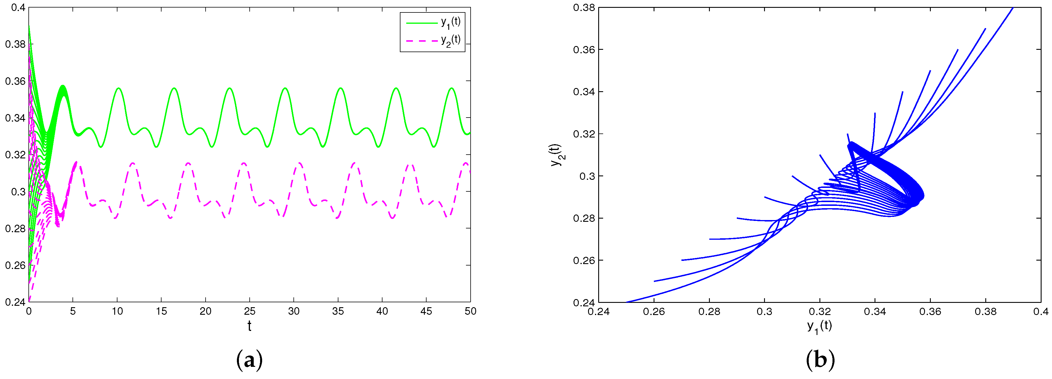
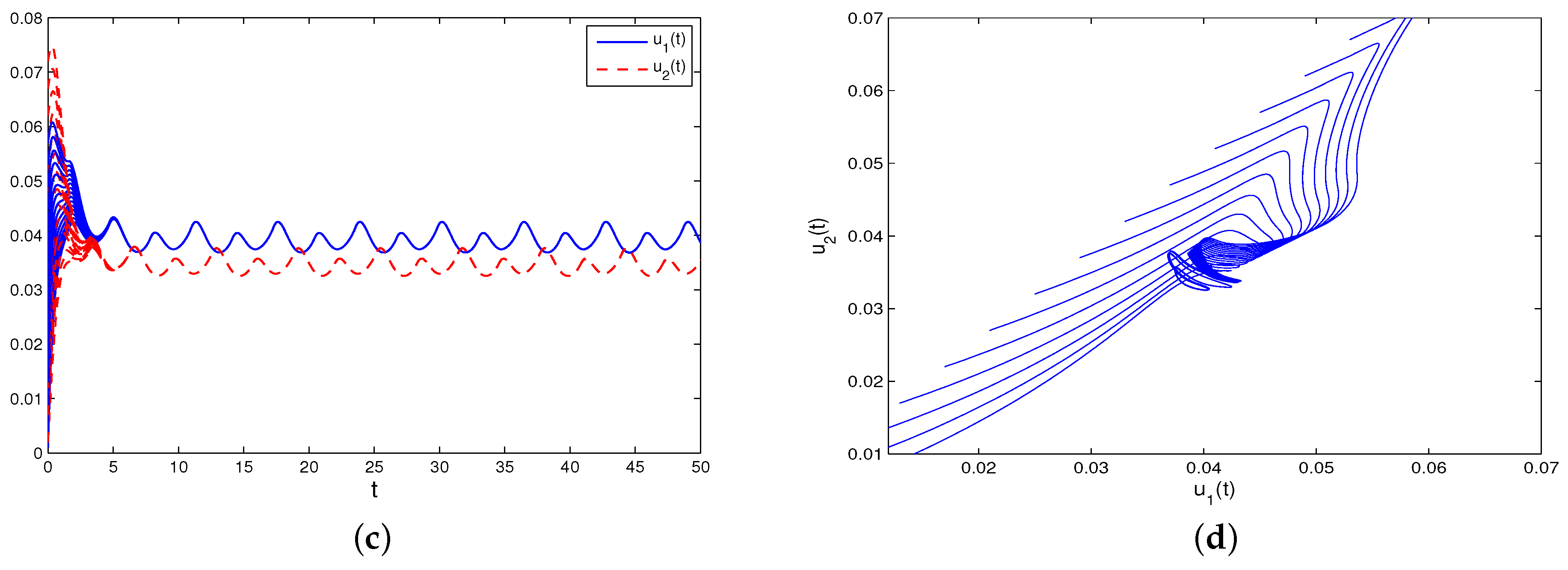
From Figure 1, one can find a permanent and globally attractive positive periodic solution for system (31).
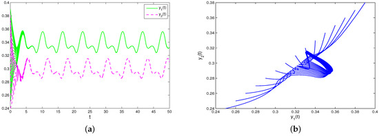
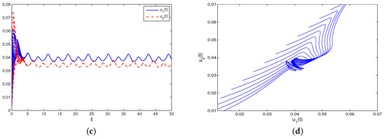
Figure 1.
Permanence, periodic solution, and global attractivity of system (31). (a,b) Permanence, periodic solution, and global attractivity of and . (c,d) Permanence, periodic solution, and global attractivity of and .
Remark 2.
The numerical simulations in Figure 1a–d illustrate that if the coefficients (intrinsic growth rates , intra-enterprise competition rate , conversion of commodity into the reproduction rate , initial productions , and feedback control coefficients ) of model (31) satisfy the conditions of Theorems 1–3, and Corollary 1, then system (31) remains stable for a long time, which means the competition and cooperation of enterprises can reach a dynamical balance, and solutions and (output of enterprises) are also uniquely remnants between the determined quantities and for a long time.
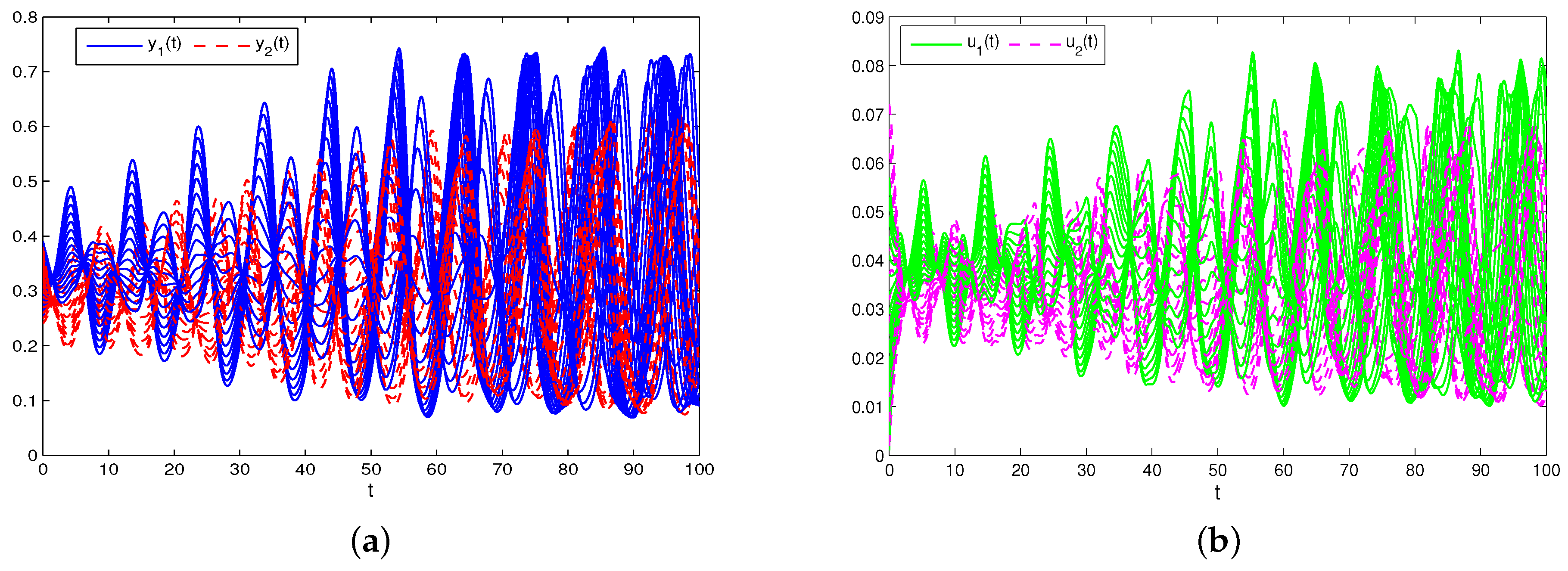
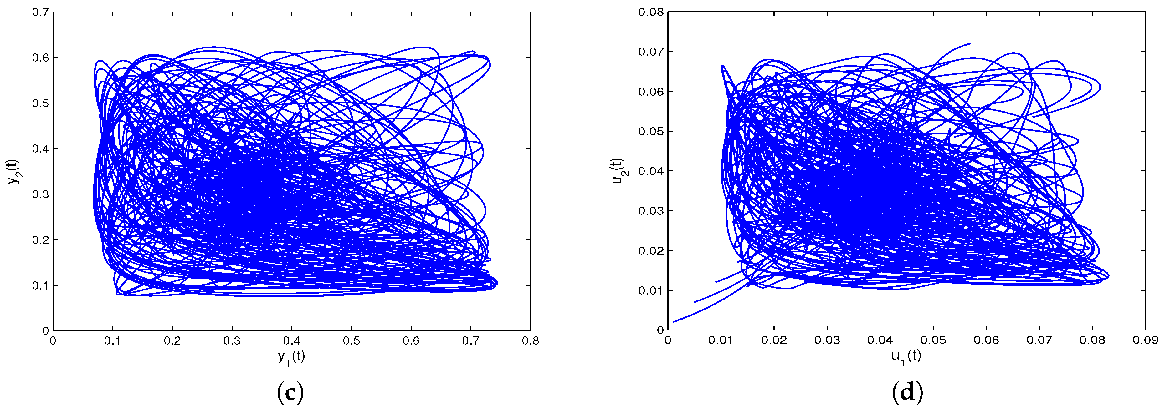
Next, we take ; then, we have
Evidently, the conditions of Theorem 3 are failed.
From Figure 2, one can find that system (31) is not globally attractive.
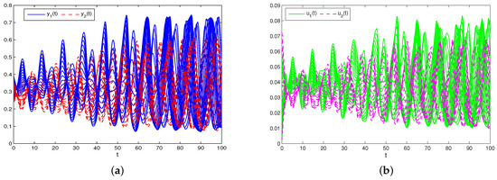
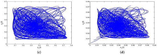
Figure 2.
Non-global attractivity of system (31). (a,c) Non-global attractivity of and . (b,d) Non-global attractivity of and .
6. Conclusions
In this study, by proposing system (6), which incorporates time-varying coefficients and feedback controls, we expanded upon existing models (1–5) and enriched the understanding of enterprise clusters. The derived conditions for dynamic behaviors in system (6) offer new insights into the growth patterns, stability, and coexistence within enterprise clusters. Hence, the derivation of conditions for dynamic behaviors in system (6) contribute to the existing body of knowledge on enterprise cluster modeling. Additionally, we can see from the conditions and results of Theorems 1–3, Corollary 1, and Example 1, that discrete time delays and feedback control coefficients and have influence on the aforementioned dynamic behaviors of model (6). In conclusion, the fate of an enterprise cluster is influenced by multiple factors, including feedback control effects, time delay effects, self-development, market saturation degree, competition power, and varying economic environments. Understanding and effectively managing these factors can help enterprises navigate challenges, seize opportunities, and achieve sustainable growth in a competitive business landscape.
Author Contributions
Conceptualization, A.M.; writing—original draft preparation, A.M. and Y.M.; writing—review and editing, A.M. and Y.M.; supervision, A.M. methodology. All authors have read and agreed to the published version of the manuscript.
Funding
This research is supported by the Talent Project of Tianchi Doctoral Program in Xinjiang Uygur Autonomous Region (No. 51052300524), National Natural Science Foundation of Xinjiang (grant no. 2021D01C067), and the Open Project of Key Laboratory of Applied Mathematics of Xinjiang Uygur Autonomous Region (grant no. 2023D04045).
Data Availability Statement
Not applicable.
Conflicts of Interest
The authors declare no conflict of interest.
References
- Tian, X.; Nie, Q. On model construction of enterprises, interactive relationship from the perspective of business ecosystem. South. Econ. J. 2006, 4, 50–57. [Google Scholar]
- Liao, M.; Xu, C.; Tang, X. Dynamical behavior for a competition and cooperation model of enterpries with two delays. Nonlinear Dyn. 2014, 75, 257–266. [Google Scholar] [CrossRef]
- Liao, M.; Xu, C.; Tang, X. Stability and Hopf bifurcation for a competition and cooperation model of two enterprises with delay. Commun. Nonlinear Sci. Numer. 2014, 19, 3845–3856. [Google Scholar] [CrossRef]
- Li, L.; Zhang, C.; Yan, X. Stability and Hopf bifurcation analysis for a two-enterprise interaction model with delays. Commun. Nonlinear Sci. Numer. Simulat. 2016, 30, 70–83. [Google Scholar] [CrossRef]
- Guerrini, L. Small delays in a competition and cooperation model of enterprises. Appl. Math. Sci. 2016, 52, 2571–2574. [Google Scholar] [CrossRef]
- Xu, C.; Shao, Y. Existence and global attractivity of periodic solution for enterprise clusters based on ecology theory with impulse. J. Appl. Math. Comput. 2012, 39, 367–384. [Google Scholar] [CrossRef]
- Xu, C.; Liao, M.; Li, P. Bifurcation control of a fractional-order delayed competition and cooperation model of two enterprises. Sci. China Technol. Sci. 2019, 62, 2130–2143. [Google Scholar] [CrossRef]
- Xu, C.; Liao, M.; Li, P.; Yuan, S. New insights on bifurcation in a fractional-order delayed competition and cooperation model of two enterprises. J. Appl. Anal. Comput. 2021, 11, 1240–1258. [Google Scholar] [CrossRef] [PubMed]
- Muhammadhaji, A.; Nureji, M. Dynamical behavior of competition and cooperation dynamical model of two enterprises. J. Quant. Econ. 2019, 36, 94–98. [Google Scholar]
- Xu, C.; Li, P.; Liao, M.; Yuan, S. New results on competition and cooperation model of two enterprises with multiple delays and feedback controls. Bound. Value Probl. 2019, 36, 12. [Google Scholar] [CrossRef]
- Lu, L.; Lian, Y.; Li, C. Dynamics for a discrete competition and cooperation model of two enterprises with multiple delays and feedback controls. Open Math. 2017, 15, 218–232. [Google Scholar] [CrossRef]
- Xu, C.; Li, P. Almost periodic solutions for a competition and cooperation model of two enterprises with time-varying delays and feedback controls. J. Appl. Math. Comput. 2017, 53, 397–411. [Google Scholar] [CrossRef]
- Nakata, Y.; Muroya, Y. Permanence for nonautonomous Lotka-Volterra cooperative systems with delays. Nonl. Anal. RWA 2010, 11, 528–534. [Google Scholar] [CrossRef]
- Zhang, Z.; Wu, J.; Wang, Z. Periodic solutions of nonautonomous stage-structured cooperative system. Comput. Math. Appl. 2004, 47, 699–706. [Google Scholar] [CrossRef]
- Gaines, R.E.; Mawhin, J.L. Coincidence degree and nonlinear differential equations. In Lecture Notes in Mathematics; Springer: Berlin/Heidelberg, Germany, 1977; Volume 568. [Google Scholar]
Disclaimer/Publisher’s Note: The statements, opinions and data contained in all publications are solely those of the individual author(s) and contributor(s) and not of MDPI and/or the editor(s). MDPI and/or the editor(s) disclaim responsibility for any injury to people or property resulting from any ideas, methods, instructions or products referred to in the content. |
© 2023 by the authors. Licensee MDPI, Basel, Switzerland. This article is an open access article distributed under the terms and conditions of the Creative Commons Attribution (CC BY) license (https://creativecommons.org/licenses/by/4.0/).