
Predicting Glycemic Control in a Small Cohort of Children with Type 1 Diabetes Using Machine Learning Algorithms

Abstract
:1. Introduction
2. Materials and Methods
2.1. Setting and Time Frame
2.2. Inclusion and Exclusion Criteria
2.3. Data Collection and Structure
2.4. Data Analysis
2.4.1. Bivariate Analysis
2.4.2. Logistic Regression
- is the output value (constrained between 0 and 1).
- is the input to the function, calculated as the weighted sum of inputs.
- is the probability that the dependent event occurred based on the linear combination of independent variables.
- is the regression coefficient for variable
- is the intercept value.
- is the true class label (0 or 1 in binary regression);
- is the predicted probability of the instance belonging to class 1.
- denotes the statistic from a bootstrap sample;
- is the original statistic, and the bias correction is given as follows:
- is the quantile function of the standard normal distribution,
- is the number of bootstrap resamples,
- I is the indicator function.
- is the statistic with the ith observation removed.
- is the average of jackknife estimates.
- is the quantile of the standard normal distribution.
2.4.3. Two-Step Cluster Algorithm
- is the number of data points in the cluster.
- corresponds to individual data points in the cluster.
- is the total number of data points.
- is the number of clusters.
- is a weight (defined as one if the datapoint I belongs to cluster j and 0 otherwise);
- is the ith data point;
- is the centroid of the jth cluster;
- is the squared Euclidean distance, which measures how far a point is from the centroid of its cluster.
- is the number of parameters in the model;
- is the number of data points in the set.
- represents the parameters of the model;
- is the probability of the data point being observed given the parameters .
- is the total number of data records in cluster .
- is the total number of continuous variables.
- is the total number of categorical variables.
- is the estimated variance of the continuous variable for the entire dataset.
- is the estimated variance of the continuous variable in cluster .
- represents the entropy-based metric for categorical variables in cluster .
- is the number of categories for the -th categorical variable [54].
- is the number of observations in cluster s where the categorical variable k takes the value of l.
- is the total number of observations where the categorical variable k takes the value of l.
- is the average distance from the sample to the other points in the same cluster.
- is the smallest average distance from the sample to the points in other clusters and minimized over clusters.
2.4.4. CART Algorithm
- represents the number of samples in child node c;
- is the total number of samples in the current node (parent node) before the split.
- is the proportion of samples reaching the leaf;
- is the error at that leaf;
- controls the trade-off between the complexity and fit of the tree.
2.4.5. Method Comparison and Agreement
2.4.6. Handling Outliers
3. Results
3.1. Bivariate Analysis
3.1.1. Demographic and Socioeconomic Characteristics
3.1.2. Disease Characteristics
3.2. Binary Logistic Regression
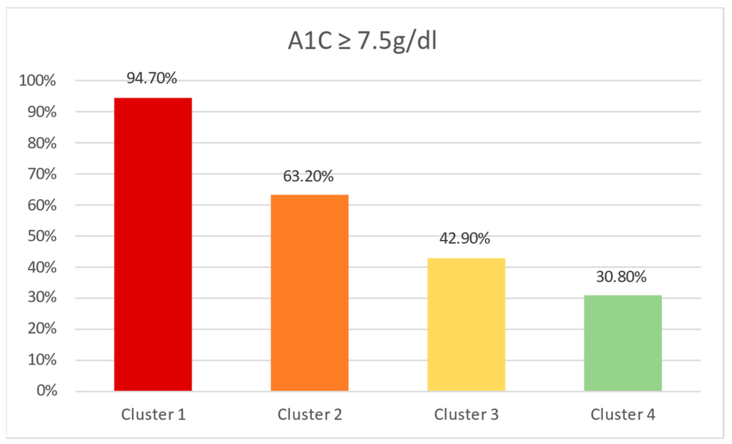
3.3. Two-Step Clustering Algorithm
3.4. CART Decision Tree
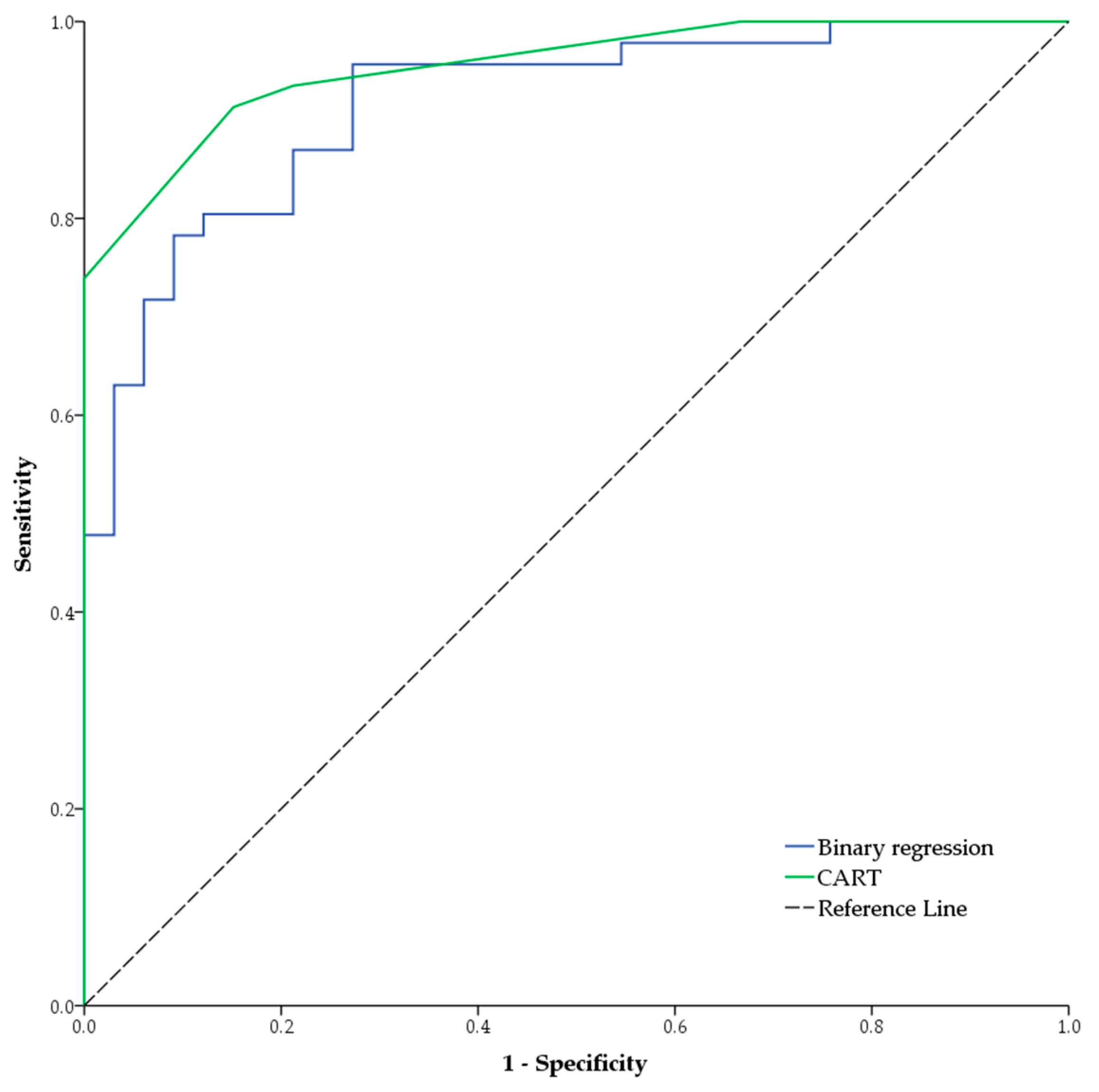
3.5. Comparison and Agreement between Methods
3.5.1. CART vs. Regression
3.5.2. Two-Step-Clustering vs. CART
3.6. Handling Outliers
4. Discussion
Strengths and Limitations
5. Conclusions
Author Contributions
Funding
Data Availability Statement
Conflicts of Interest
Appendix A. Results Obtained through Bivariate Analysis
References
- DiMeglio, L.A.; Evans-Molina, C.; Oram, R.A. Type 1 Diabetes. Lancet 2018, 391, 2449–2462. [Google Scholar] [CrossRef] [PubMed]
- Huo, L.; Harding, J.L.; Peeters, A.; Shaw, J.E.; Magliano, D.J. Life Expectancy of Type 1 Diabetic Patients during 1997–2010: A National Australian Registry-Based Cohort Study. Diabetologia 2016, 59, 1177–1185. [Google Scholar] [CrossRef] [PubMed]
- Petrie, D.; Lung, T.W.C.; Rawshani, A.; Palmer, A.J.; Svensson, A.-M.; Eliasson, B.; Clarke, P. Recent Trends in Life Expectancy for People with Type 1 Diabetes in Sweden. Diabetologia 2016, 59, 1167–1176. [Google Scholar] [CrossRef] [PubMed]
- American Diabetes Association Professional Practice Committee. 2. Classification and Diagnosis of Diabetes: Standards of Medical Care in Diabetes—2020. Diabetes Care 2020, 43 (Suppl. S1), S14–S31. [Google Scholar] [CrossRef]
- Cho, N.H.; Shaw, J.E.; Karuranga, S.; Huang, Y.; da Rocha Fernandes, J.D.; Ohlrogge, A.W.; Malanda, B. IDF Diabetes Atlas: Global Estimates of Diabetes Prevalence for 2017 and Projections for 2045. Diabetes Res Clin Pr. 2018, 138, 271–281. [Google Scholar] [CrossRef] [PubMed]
- Heier, M.; Margeirsdottir, H.D.; Brunborg, C.; Hanssen, K.F.; Dahl-Jørgensen, K.; Seljeflot, I. Inflammation in Childhood Type 1 Diabetes; Influence of Glycemic Control. Atherosclerosis 2015, 238, 33–37. [Google Scholar] [CrossRef]
- Gourgari, E.; Dabelea, D.; Rother, K. Modifiable Risk Factors for Cardiovascular Disease in Children with Type 1 Diabetes: Can Early Intervention Prevent Future Cardiovascular Events? Curr. Diabetes Rep. 2017, 17, 134. [Google Scholar] [CrossRef]
- Hafez, M.; Hassan, M.; Musa, N.; Abdel Atty, S.; Azim, S.A. Vitamin D Status in Egyptian Children with Type 1 Diabetes and the Role of Vitamin D Replacement in Glycemic Control. J. Pediatr. Endocrinol. Metab. 2017, 30, 389–394. [Google Scholar] [CrossRef]
- Jaiswal, M.; Divers, J.; Dabelea, D.; Isom, S.; Bell, R.A.; Martin, C.L.; Pettitt, D.J.; Saydah, S.; Pihoker, C.; Standiford, D.A.; et al. Prevalence of and Risk Factors for Diabetic Peripheral Neuropathy in Youth with Type 1 and Type 2 Diabetes: SEARCH for Diabetes in Youth Study. Diabetes Care 2017, 40, 1226–1232. [Google Scholar] [CrossRef]
- Savastio, S.; Cadario, F.; Genoni, G.; Bellomo, G.; Bagnati, M.; Secco, G.; Picchi, R.; Giglione, E.; Bona, G. Vitamin D Deficiency and Glycemic Status in Children and Adolescents with Type 1 Diabetes Mellitus. PLoS ONE 2016, 11, e0162554. [Google Scholar] [CrossRef]
- Ordooei, M.; Shojaoddiny-Ardekani, A.; Hoseinipoor, S.H.; Miroliai, M.; Zare-Zardini, H. Effect of Vitamin D on HbA1c Levels of Children and Adolescents with Diabetes Mellitus Type 1. Minerva Pediatr. 2017, 69, 391–395. [Google Scholar] [CrossRef]
- Rewers, M.; Ludvigsson, J. Environmental Risk Factors for Type 1 Diabetes. Lancet 2016, 387, 2340–2348. [Google Scholar] [CrossRef]
- Mohammad, H.; Farghaly, H.; Metwalley, K.; Monazea, E.; Abd El-Hafeez, H. Predictors of Glycemic Control in Children with Type 1 Diabetes Mellitus in Assiut-Egypt. Indian. J. Endocrinol. Metab. 2012, 16, 796. [Google Scholar] [CrossRef]
- Niba, L.L.; Aulinger, B.; Mbacham, W.F.; Parhofer, K.G. Predictors of Glucose Control in Children and Adolescents with Type 1 Diabetes: Results of a Cross-Sectional Study in Cameroon. BMC Res. Notes 2017, 10, 207. [Google Scholar] [CrossRef] [PubMed]
- Chiang, J.L.; Kirkman, M.S.; Laffel, L.M.B.; Peters, A.L. Type 1 Diabetes Through the Life Span: A Position Statement of the American Diabetes Association. Diabetes Care 2014, 37, 2034–2054. [Google Scholar] [CrossRef] [PubMed]
- DiMeglio, L.A.; Acerini, C.L.; Codner, E.; Craig, M.E.; Hofer, S.E.; Pillay, K.; Maahs, D.M. ISPAD Clinical Practice Consensus Guidelines 2018: Glycemic Control Targets and Glucose Monitoring for Children, Adolescents, and Young Adults with Diabetes. Pediatr. Diabetes 2018, 19, 105–114. [Google Scholar] [CrossRef]
- Cutfield, S.W.; Derraik, J.G.B.; Reed, P.W.; Hofman, P.L.; Jefferies, C.; Cutfield, W.S. Early Markers of Glycaemic Control in Children with Type 1 Diabetes Mellitus. PLoS ONE 2011, 6, e25251. [Google Scholar] [CrossRef] [PubMed]
- World Health Organisation. WHO Expert Committee on Diabetes Mellitus: Second Report. World Health Organ. Tech. Rep. Ser. 1980, 646, 1–80. [Google Scholar]
- Urbach, S.L.; LaFranchi, S.; Lambert, L.; Lapidus, J.A.; Daneman, D.; Becker, T.M. Predictors of Glucose Control in Children and Adolescents with Type 1 Diabetes Mellitus. Pediatr. Diabetes 2005, 6, 69–74. [Google Scholar] [CrossRef] [PubMed]
- Eurostat. International Standard Classification of Education (ISCED). Available online: https://ec.europa.eu/eurostat/statistics-explained/index.php?title=International_Standard_Classification_of_Education_(ISCED) (accessed on 22 September 2023).
- Beck, R.W.; Tamborlane, W.V.; Bergenstal, R.M.; Miller, K.M.; DuBose, S.N.; Hall, C.A. The T1D Exchange Clinic Registry. J. Clin. Endocrinol. Metab. 2012, 97, 4383–4389. [Google Scholar] [CrossRef] [PubMed]
- Samuelsson, U.; Steineck, I.; Gubbjornsdottir, S. A High Mean-HbA1c Value 3-15 Months after Diagnosis of Type 1 Diabetes in Childhood Is Related to Metabolic Control, Macroalbuminuria, and Retinopathy in Early Adulthood-a Pilot Study Using Two Nation-Wide Population Based Quality Registries. Pediatr. Diabetes 2014, 15, 229–235. [Google Scholar] [CrossRef]
- Springer, D.; Dziura, J.; Tamborlane, W.V.; Steffen, A.T.; Ahern, J.H.; Vincent, M.; Weinzimer, S.A. Optimal Control of Type 1 Diabetes Mellitus in Youth Receiving Intensive Treatment. J. Pediatr. 2006, 149, 227–232. [Google Scholar] [CrossRef] [PubMed]
- Carter, P.J.; Cutfield, W.S.; Hofman, P.L.; Gunn, A.J.; Wilson, D.A.; Reed, P.W.; Jefferies, C. Ethnicity and Social Deprivation Independently Influence Metabolic Control in Children with Type 1 Diabetes. Diabetologia 2008, 51, 1835–1842. [Google Scholar] [CrossRef]
- Gallegos-Macias, A.R.; Macias, S.R.; Kaufman, E.; Skipper, B.; Kalishman, N. Relationship between Glycemic Control, Ethnicity and Socioeconomic Status in Hispanic and White Non-Hispanic Youths with Type 1 Diabetes Mellitus. Pediatr. Diabetes 2003, 4, 19–23. [Google Scholar] [CrossRef]
- Overstreet, S.; Holmes, C.S.; Dunlap, W.P.; Frentz, J. Sociodemographic Risk Factors to Disease Control in Children with Diabetes. Diabet. Med. 1997, 14, 153–157. [Google Scholar] [CrossRef]
- Hassan, K.; Loar, R.; Anderson, B.J.; Heptulla, R.A. The Role of Socioeconomic Status, Depression, Quality of Life, and Glycemic Control in Type 1 Diabetes Mellitus. J. Pediatr. 2006, 149, 526–531. [Google Scholar] [CrossRef] [PubMed]
- Fredheim, S.; Johannesen, J.; Johansen, A.; Lyngsøe, L.; Rida, H.; Andersen, M.L.M.; Lauridsen, M.H.; Hertz, B.; Birkebæk, N.H.; Olsen, B.; et al. Diabetic Ketoacidosis at the Onset of Type 1 Diabetes Is Associated with Future HbA1c Levels. Diabetologia 2013, 56, 995–1003. [Google Scholar] [CrossRef]
- Duca, L.M.; Wang, B.; Rewers, M.; Rewers, A. Diabetic Ketoacidosis at Diagnosis of Type 1 Diabetes Predicts Poor Long-Term Glycemic Control. Diabetes Care 2017, 40, 1249–1255. [Google Scholar] [CrossRef] [PubMed]
- Viswanathan, V.; Sneeringer, M.R.; Miller, A.; Eugster, E.A.; DiMeglio, L.A. The Utility of Hemoglobin A1c at Diagnosis for Prediction of Future Glycemic Control in Children with Type 1 Diabetes. Diabetes Res. Clin. Pr. 2011, 92, 65–68. [Google Scholar] [CrossRef]
- Shalitin, S.; Phillip, M. Which Factors Predict Glycemic Control in Children Diagnosed with Type 1 Diabetes before 6.5 Years of Age? Acta Diabetol. 2012, 49, 355–362. [Google Scholar] [CrossRef] [PubMed]
- Rudberg, S.; Ullman, E.; Dahlquist, G. Relationship between Early Metabolic Control and the Development of Microalbuminuria? A Longitudinal Study in Children with Type 1 (Insulin-Dependent) Diabetes Mellitus. Diabetologia 1993, 36, 1309–1314. [Google Scholar] [CrossRef]
- Svensson, M.; Eriksson, J.W.; Dahlquist, G. Early Glycemic Control, Age at Onset, and Development of Microvascular Complications in Childhood-Onset Type 1 Diabetes. Diabetes Care 2004, 27, 955–962. [Google Scholar] [CrossRef]
- Borghi, E.; de Onis, M.; Garza, C.; Van den Broeck, J.; Frongillo, E.A.; Grummer-Strawn, L.; Van Buuren, S.; Pan, H.; Molinari, L.; Martorell, R.; et al. Construction of the World Health Organization Child Growth Standards: Selection of Methods for Attained Growth Curves. Stat. Med. 2006, 25, 247–265. [Google Scholar] [CrossRef] [PubMed]
- Guy, J.; Ogden, L.; Wadwa, R.P.; Hamman, R.F.; Mayer-Davis, E.J.; Liese, A.D.; D’Agostino, R.; Marcovina, S.; Dabelea, D. Lipid and Lipoprotein Profiles in Youth with and without Type 1 Diabetes. Diabetes Care 2009, 32, 416–420. [Google Scholar] [CrossRef] [PubMed]
- McKinney, P.A.; Feltbower, R.G.; Stephenson, C.R. Children and Young People with Diabetes in Yorkshire: A Population Based Clinical Audit of Patient Data 2005/6. Diabet. Med. 2008, 25, 1276–1282. [Google Scholar] [CrossRef] [PubMed]
- Hilliard, M.E.; Wu, Y.P.; Rausch, J.; Dolan, L.M.; Hood, K.K. Predictors of Deteriorations in Diabetes Management and Control in Adolescents with Type 1 Diabetes. J. Adolesc. Health 2013, 52, 28–34. [Google Scholar] [CrossRef]
- Hughes, J.W.; Riddlesworth, T.D.; DiMeglio, L.A.; Miller, K.M.; Rickels, M.R.; McGill, J.B. Autoimmune Diseases in Children and Adults with Type 1 Diabetes from the T1D Exchange Clinic Registry. J. Clin. Endocrinol. Metab. 2016, 101, 4931–4937. [Google Scholar] [CrossRef]
- Rewers, A. Predictors of Acute Complications in Children with Type 1 Diabetes. JAMA 2002, 287, 2511. [Google Scholar] [CrossRef]
- Fritsch, M.; Rosenbauer, J.; Schober, E.; Neu, A.; Placzek, K.; Holl, R.W. Predictors of Diabetic Ketoacidosis in Children and Adolescents with Type 1 Diabetes. Experience from a Large Multicentre Database. Pediatr. Diabetes 2011, 12 Pt 1, 307–312. [Google Scholar] [CrossRef]
- Guglielmi, C.; Leslie, R.D.; Pozzilli, P. Epidemiology and Risk Factors of Type 1 Diabetes. In Diabetes. Epidemiology, Genetics, Pathogenesis, Diagnosis, Prevention, and Treatment; Springer: Berlin/Heidelberg, Germany, 2018; pp. 41–54. [Google Scholar] [CrossRef]
- Virk, S.A.; Donaghue, K.C.; Cho, Y.H.; Benitez-Aguirre, P.; Hing, S.; Pryke, A.; Chan, A.; Craig, M.E. Association between HbA 1c Variability and Risk of Microvascular Complications in Adolescents with Type 1 Diabetes. J. Clin. Endocrinol. Metab. 2016, 101, 3257–3263. [Google Scholar] [CrossRef]
- Alemzadeh, R.; Berhe, T.; Wyatt, D.T. Flexible Insulin Therapy with Glargine Insulin Improved Glycemic Control and Reduced Severe Hypoglycemia among Preschool-Aged Children with Type 1 Diabetes Mellitus. Pediatrics 2005, 115, 1320–1324. [Google Scholar] [CrossRef]
- Singh, K.; Martinell, M.; Luo, Z.; Espes, D.; Stålhammar, J.; Sandler, S.; Carlsson, P.-O. Cellular Immunological Changes in Patients with LADA Are a Mixture of Those Seen in Patients with Type 1 and Type 2 Diabetes. Clin. Exp. Immunol. 2019, 197, 64–73. [Google Scholar] [CrossRef] [PubMed]
- Cheng, Y.; Yu, W.; Zhou, Y.; Zhang, T.; Chi, H.; Xu, C. Novel Predictor of the Occurrence of DKA in T1DM Patients without Infection: A Combination of Neutrophil/Lymphocyte Ratio and White Blood Cells. Open Life Sci. 2021, 16, 1365–1376. [Google Scholar] [CrossRef] [PubMed]
- Scutca, A.-C.; Nicoară, D.-M.; Mărăzan, M.; Brad, G.-F.; Mărginean, O. Neutrophil-to-Lymphocyte Ratio Adds Valuable Information Regarding the Presence of DKA in Children with New-Onset T1DM. J. Clin. Med. 2022, 12, 221. [Google Scholar] [CrossRef] [PubMed]
- Baghersalimi, A.; Koohmanaee, S.; Darbandi, B.; Farzamfard, V.; Hassanzadeh Rad, A.; Zare, R.; Tabrizi, M.; Dalili, S. Platelet Indices Alterations in Children with Type 1 Diabetes Mellitus. J. Pediatr. Hematol. Oncol. 2019, 41, e227–e232. [Google Scholar] [CrossRef]
- Söbü, E.; Demir Yenigürbüz, F.; Özçora, G.D.K.; Köle, M.T. Evaluation of the Impact of Glycemic Control on Mean Platelet Volume and Platelet Activation in Children with Type 1 Diabetes. J. Trop. Pediatr. 2022, 68, fmac063. [Google Scholar] [CrossRef]
- Pirgon, O.; Asya Tanju, I.; Alev Erikci, A. Association of Mean Platelet Volume between Glucose Regulation in Children with Type 1 Diabetes. J. Trop. Pediatr. 2007, 55, 63–64. [Google Scholar] [CrossRef]
- Hastie, T.; Tibshirani, R.; Friedman, J. The Elements of Statistical Learning: Data Mining, Inference, and Prediction, 2nd ed.; Springer: Stanford, CA, USA, 2008. [Google Scholar]
- Lin, Y.-Q.; Zhang, Y.-S.; Tian, G.-L.; Ma, C.-X. Fast QLB Algorithm and Hypothesis Tests in Logistic Model for Ophthalmologic Bilateral Correlated Data. J. Biopharm. Stat. 2021, 31, 91–107. [Google Scholar] [CrossRef]
- Davison, A.C.; Hinkley, D.V. Bootstrap Methods and Their Application; Cambridge University Press: Cambridge, UK, 1997. [Google Scholar] [CrossRef]
- Carpenter, J.; Bithell, J. Bootstrap Confidence Intervals: When, Which, What? A Practical Guide for Medical Statisticians. Stat. Med. 2000, 19, 1141–1164. [Google Scholar] [CrossRef]
- Șchiopu, D. Applying TwoStep Cluster Analysis for Identifying Bank Customer’s Profile. Econ. Insights—Trends Chall. 2010, 62, 66–75. [Google Scholar]
- Tan, P.-N.; Steinbach, M. Introduction to Data Mining, 2nd ed.; Pearson: London, UK, 2018. [Google Scholar]
- Jain, A.K.; Murty, M.N.; Flynn, P.J. Data Clustering. ACM Comput. Surv. 1999, 31, 264–323. [Google Scholar] [CrossRef]
- Rousseeuw, P.J. Silhouettes: A Graphical Aid to the Interpretation and Validation of Cluster Analysis. J. Comput. Appl. Math. 1987, 20, 53–65. [Google Scholar] [CrossRef]
- Conn, D.; Ramirez, C.M. Random Forests and Fuzzy Forests in Biomedical Research. In Computational Social Science; Cambridge University Press: Cambridge, UK, 2016; pp. 168–196. [Google Scholar] [CrossRef]
- James, G.; Witten, D.; Hastie, T.; Tibshirani, R. An Introduction to Statistical Learning with Applications in R, 2nd ed.; Springer: Berlin/Heidelberg, Germany, 2013. [Google Scholar]
- Landis, J.R.; Koch, G.G. The Measurement of Observer Agreement for Categorical Data. Biometrics 1977, 33, 159. [Google Scholar] [CrossRef]
- Noorani, M.; Ramaiya, K.; Manji, K. Glycaemic Control in Type 1 Diabetes Mellitus among Children and Adolescents in a Resource Limited Setting in Dar Es Salaam—Tanzania. BMC Endocr. Disord. 2016, 16, 29. [Google Scholar] [CrossRef] [PubMed]
- Dalmaijer, E.S.; Nord, C.L.; Astle, D.E. Statistical Power for Cluster Analysis. BMC Bioinform. 2022, 23, 205. [Google Scholar] [CrossRef]
- Rohan, J.M.; Delamater, A.; Pendley, J.S.; Dolan, L.; Reeves, G.; Drotar, D. Identification of Self-Management Patterns in Pediatric Type 1 Diabetes Using Cluster Analysis. Pediatr. Diabetes 2011, 12, 611–618. [Google Scholar] [CrossRef] [PubMed]
- Lu, M.-Y.; Liu, T.-W.; Liang, P.-C.; Huang, C.-I.; Tsai, Y.-S.; Tsai, P.-C.; Ko, Y.-M.; Wang, W.-H.; Lin, C.-C.; Chen, K.-Y.; et al. Decision Tree Algorithm Predicts Hepatocellular Carcinoma among Chronic Hepatitis C Patients Following Viral Eradication. Am. J. Cancer Res. 2023, 13, 190–203. [Google Scholar]
- Machuca, C.; Vettore, M.V.; Krasuska, M.; Baker, S.R.; Robinson, P.G. Using Classification and Regression Tree Modelling to Investigate Response Shift Patterns in Dentine Hypersensitivity. BMC Med. Res. Methodol. 2017, 17, 120. [Google Scholar] [CrossRef]
- Althnian, A.; AlSaeed, D.; Al-Baity, H.; Samha, A.; Dris, A.B.; Alzakari, N.; Abou Elwafa, A.; Kurdi, H. Impact of Dataset Size on Classification Performance: An Empirical Evaluation in the Medical Domain. Appl. Sci. 2021, 11, 796. [Google Scholar] [CrossRef]
- Van der Ploeg, T.; Austin, P.C.; Steyerberg, E.W. Modern Modelling Techniques Are Data Hungry: A Simulation Study for Predicting Dichotomous Endpoints. BMC Med. Res. Methodol. 2014, 14, 137. [Google Scholar] [CrossRef]
- Reininger, B.M.; Lopez, J.; Zolezzi, M.; Lee, M.; Mitchell-Bennett, L.A.; Xu, T.; Park, S.K.; Saldana, M.V.; Perez, L.; Payne, L.Y.; et al. Participant Engagement in a Community Health Worker-Delivered Intervention and Type 2 Diabetes Clinical Outcomes: A Quasiexperimental Study in MexicanAmericans. BMJ Open 2022, 12, e063521. [Google Scholar] [CrossRef] [PubMed]
- Gill, A.; Gothard, M.D.; Briggs Early, K. Glycemic Outcomes among Rural Patients in the Type 1 Diabetes T1D Exchange Registry, January 2016–March 2018: A Cross-Sectional Cohort Study. BMJ Open Diabetes Res Care 2022, 10, e002564. [Google Scholar] [CrossRef]
- Svoren, B.M.; Volkening, L.K.; Butler, D.A.; Moreland, E.C.; Anderson, B.J.; Laffel, L.M.B. Temporal Trends in the Treatment of Pediatric Type 1 Diabetes and Impact on Acute Outcomes. J. Pediatr. 2007, 150, 279–285. [Google Scholar] [CrossRef] [PubMed]
- Holl, R.; Swift, P.; Mortensen, H.; Lynggaard, H.; Hougaard, P.; Aanstoot, H.-J.; Chiarelli, F.; Daneman, D.; Danne, T.; Dorchy, H.; et al. Insulin Injection Regimens and Metabolic Control in an International Survey of Adolescents with Type 1 Diabetes over 3 Years: Results from the Hvidore Study Group. Eur. J. Pediatr. 2003, 162, 22–29. [Google Scholar] [CrossRef] [PubMed]


| Variable | Raw Data | Processed Variable Type (Explanation) | Ref. |
|---|---|---|---|
| Demographic characteristics | |||
| Gender | Dichotomous | Dichotomous (Male/Female) | [14,19] |
| Paternal level of education | Ordinal (ISCED 0–7) | Dichotomous (ISCED > 4 vs. ISCED ≤ 4) Higher education vs. no higher education | [13,14,21,22,23,24,25,26,27] |
| Maternal level of education | |||
| Family income | Continuous | Categorial (High/average/low compared to the average income in Romania for 2018) | |
| Living conditions | Dichotomous | Dichotomous (Rural/Urban) | |
| Disease characteristics | |||
| Family history of diabetes | Dichotomous | Dichotomous (Yes/No) | [14,21,28] |
| Type of onset | Nominal | Categorial (Asymptomatic or symptomatic with no ketoacidosis/ Mild or moderate ketoacidosis/ severe ketoacidosis) | [28,29] |
| A1C at onset | Continuous | Dihotomous (<7.5 g/dL/≥7.5 g/dL) | [22,30,31,32,33] |
| Age of onset | Continuous | Categorial (<5 years/5–10 years/>10 years) | [13,22,28] |
| BMI at onset (Z-score, according to WHO 2007 growth reference data [34]) | Continuous | Continuous, Categorical (underweight/normal weight/overweight or obese) according to WHO Reference values for BMI Z-score (<2; 2–1; >1) | [13,14,35] |
| Disease duration | Continuous | Continuous | [24,36,37] |
| Identified associated autoimmune diseases | Nominal | Dichotomous (Yes/No) | [38] |
| Episodes of hypoglicemia | Discrete | Dichotomous (Yes/No) | [21,39] |
| Episodes of ketoacidosis (excluding onset [39]) | Discrete | Dichotomous (Yes/No) | [39,40] |
| Episodes of viral infections | Discrete | Dichotomous (Yes/No) | [41] |
| Episodes of bacterial infections | Discrete | Dichotomous (Yes/No) | |
| Episodes of microalbuminuria | Discrete | Dichotomous (Yes/No) | [21,32,42] |
| Serum Cholesterol (last documented value) | Continuous | Dihotomous (≥200 mg/dL/<200 mg/dL) | [13,35] |
| Serum Triglycerides (last documented value) | Continuous | Dihotomous (≥150 mg/dL/<150 mg/dL) | |
| Insulin regimen | Nominal | Dichotomous (Regimen 1/Regimen 2—explained in text) | [13,14,43] |
| Neutrophil to lymphocyte ratio | Continuous | Continuous | [44,45,46] |
| Mean platelet volume | Continuous | Continuous | [47,48,49] |
| Variable | Categories | Frequency of Good Glycemic Control (% of Category) | Frequency of Poor Glycemic Control (% of Category) | Total (% of Grand Total) | p-Value |
|---|---|---|---|---|---|
| Gender | Male | 22 (48.9%) | 23 (51.1%) | 45 (57%) | 0.14 |
| Female | 11 (32.4%) | 23 (67.6%) | 34 (43%) | ||
| Family income | High | 8 (80%) | 2 (20%) | 10 (12.7%) | <0.01 |
| Average | 18 (45%) | 22 (55%) | 40 (50.6%) | ||
| Low | 7 (24.1%) | 22 (75.9%) | 29 (36.7%) | ||
| Living Environment | Urban | 26 (50%) | 26 (50%) | 52 (65.8%) | 0.04 |
| Rural | 7 (25.9%) | 20 (74.1%) | 27 (34.2%) | ||
| Maternal education | ≤ISCED 4 | 24 (36.4%) | 42 (63.6%) | 66 (83.5%) | 0.028 |
| >ISCED 4 | 9 (69.2%) | 4 (30.8%) | 13 (16.5%) | ||
| Paternal education | ≤ISCED 4 | 27 (39.1%) | 42 (60.9%) | 69 (87.3%) | 0.305 |
| >ISCED 4 | 6 (60%) | 4 (40%) | 10 (12.7%) |
| Variable | Categories | Frequency of Good Glycemic Control (% of Category) | Frequency of Poor Glycemic Control (% of Category) | Total (% of Grand Total) | p-Value |
|---|---|---|---|---|---|
| Family history of diabetes | Yes | 7 (38.9%) | 11 (61.1%) | 18 (22.8%) | 0.778 |
| No | 26 (42.6%) | 35 (57.4%) | 61 (77.2%) | ||
| Type of onset (Ketoacidosis severity) | None | 5 (62.5%) | 3 (37.5%) | 8 (10.1%) | 0.384 |
| Mild/moderate | 23 (39.7%) | 35 (60.3%) | 58 (73.4%) | ||
| Severe | 5 (38.5%) | 8 (61.5%) | 13 (16.5%) | ||
| A1C at onset | <7.5 g/dL | 8 (80%) | 2 (20%) | 10 (12.7%) | 0.011 |
| ≥7.5 g/dL | 25 (36.2%) | 44 (63.8%) | 69 (87.3%) | ||
| Age of onset | <5 years | 6 (68.4%) | 13 (31.6%) | 19 (24.7%) | 0.275 |
| 5–10 years | 10 (34.5%) | 19 (65.5%) | 29 (37.7%) | ||
| >10 years | 15 (51.7%) | 14 (48.3%) | 29 (37.7%) | ||
| Nutritional status at onset | Underweight | 11 (64.7%) | 6 (35.3%) | 17 (21.5%) | 0.08 |
| Normal weight | 18 (37.5%) | 30 (62.5%) | 48 (60.8%) | ||
| Overweight/obese | 4 (28.6%) | 10 (71.4%) | 14 (17.7%) | ||
| Autoimmune diseases | Yes | 2 (33.3%) | 4 (66.7%) | 6 (7.6%) | 1.0 |
| No | 31 (42.5%) | 42 (57.5%) | 73 (92.4%) | ||
| Hypoglicemia episodes | Yes | 4 (36.4%) | 7 (63.6%) | 11 (13.9%) | 0.754 |
| No | 29 (42.6%) | 39 (57.4%) | 68 (86.1%) | ||
| Ketoacidosis episodes | Yes | 0 (0%) | 15 (100%) | 15 (19%) | <0.01 |
| No | 33 (51.6%) | 31 (48.4%) | 64 (81%) | ||
| Viral infections | Yes | 11 (30.6%) | 25 (69.4%) | 36 (45.6%) | 0.064 |
| No | 22 (51.2%) | 21 (48.8%) | 43 (54.4%) | ||
| Bacterial infections | Yes | 11 (32. 4%) | 23 (67.6%) | 34 (43%) | 0.140 |
| No | 22 (48.9%) | 23 (51.1%) | 45 (57%) | ||
| Microalbuminuria | Yes | 8 (32%) | 17 (68%) | 25 (31.6%) | 0.231 |
| No | 25 (46.3%) | 29 (53.7%) | 54 (68.4%) | ||
| Serum Cholesterol | ≥200 mg/dL | 3 (12%) | 22 (88%) | 25 (31.6%) | <0.01 |
| <200 mg/dL | 30 (55.6%) | 24 (44.4%) | 54 (68.4%) | ||
| Serum Triglycerides | ≥150 mg/dL | 2 (15.4%) | 11 (84.6%) | 13 (16.5%) | 0.035 |
| <150 mg/dL | 31 (47%) | 35 (53%) | 66 (83.5%) | ||
| Insulin Regimen | 1 | 12 (34.3%) | 23 (65.7%) | 35 (44.3%) | 0.229 |
| 2 | 21 (47.7%) | 23 (52.3%) | 44 (55.7%) |
| Variable | Descriptive Parameter | Glycemic Control | p-Value | |
|---|---|---|---|---|
| Good | Poor | |||
| Disease duration (months) | Mean | 68.09 | 90.65 | 0.04 |
| StdDev | 57.78 | 58.27 | ||
| IQR | 64 | 87 | ||
| MIN | 6 | 7 | ||
| MAX | 252 | 252 | ||
| 95%CI | 47.57–88.55 | 73.35–107.96 | ||
| BMI Z-score | Mean | −1.32 | −0.32 | 0.01 |
| StdDev | 1.55 | 1.72 | ||
| IQR | 2.47 | 2.52 | ||
| MIN | −3.91 | −4.61 | ||
| MAX | 1.59 | 2.93 | ||
| 95%CI | −1.87–−0.77 | −0.83–0.19 | ||
| NLR | Mean | 1.91 | 1.73 | 0.477 |
| StdDev | 1.28 | 1 | ||
| IQR | 0.97 | 1.02 | ||
| MIN | 0.55 | 0.52 | ||
| MAX | 7.15 | 5.09 | ||
| 95%CI | 1.46–2.37 | 1.43–2.03 | ||
| MPV (fL) | Mean | 10.55 | 10.67 | 0.62 |
| StdDev | 0.9 | 1.24 | ||
| IQR | 1 | 1.35 | ||
| MIN | 8.7 | 7.9 | ||
| MAX | 12.8 | 13.6 | ||
| 95%CI | 10.22–10.87 | 10.3–11.04 | ||
| Variable | β | p | BCa 95% CI for β | |
|---|---|---|---|---|
| Lower | Higher | |||
| Ketoacidosis episodes (X1) | 21.1 | <0.01 | 17.62 | 39.2 |
| A1C at onset ≥ 7.5 g/dL (X2) | 3.12 | <0.01 | 0.38 | 30.25 |
| Family income low or average (X3) | 2.73 | 0.018 | 0.32 | 57.02 |
| Cholesterol ≥ 200 mg/dL (X4) | 2.43 | 0.029 | 0.15 | 38.74 |
| BMI Z-score (mean-centered) (X5) | 0.58 | <0.01 | 0.1 | 1.94 |
| Constant | −5.57 | <0.01 | −24.84 | −5.08 |
| Variable | Category | Cluster 1 | Cluster 2 | Cluster 3 | Cluster 4 | Predictor Importance |
|---|---|---|---|---|---|---|
| Count | - | 19 (24.1%) | 19 (24.1%) | 28 (35.4%) | 13 (16.5%) | - |
| Higher maternal education | No | 19 (100%) | 19 (100%) | 28 (100%) | 0 (0%) | 1 |
| Yes | 0 (0%) | 0 (0%) | 0 (0%) | 13 (100%) | ||
| Living environment | Rural | 8 (42.1%) | 19 (100%) | 0 (0%) | 0 (0%) | 0.73 |
| Urban | 11 (57.9%) | 0 (0%) | 28 (100%) | 13 (100%) | ||
| Family income | Low | 9 (47.4%) | 11 (57.9%) | 9 (31.1%) | 0 (0%) | 0.67 |
| Average | 10 (52.6$) | 8 (42.1%) | 19 (67.9%) | 3 (23.1%) | ||
| High | 0 (0%) | 0 (0%) | 0 (0%) | 10 (76.9%) | ||
| Ketoacidosis episodes | Yes | 15 (78.9%) | 0 (0%) | 0 (0%) | 0 (0%) | 0.73 |
| No | 4 (21.1%) | 19 (100%) | 28 (100%) | 13 (100%) | ||
| Elevated triglycerides | Yes | 12 (63.2%) | 0 | 0 | 1 (7.7%) | 0.49 |
| No | 7 (36.8%) | 19 (100%) | 28 (100%) | 12 (92.3%) |
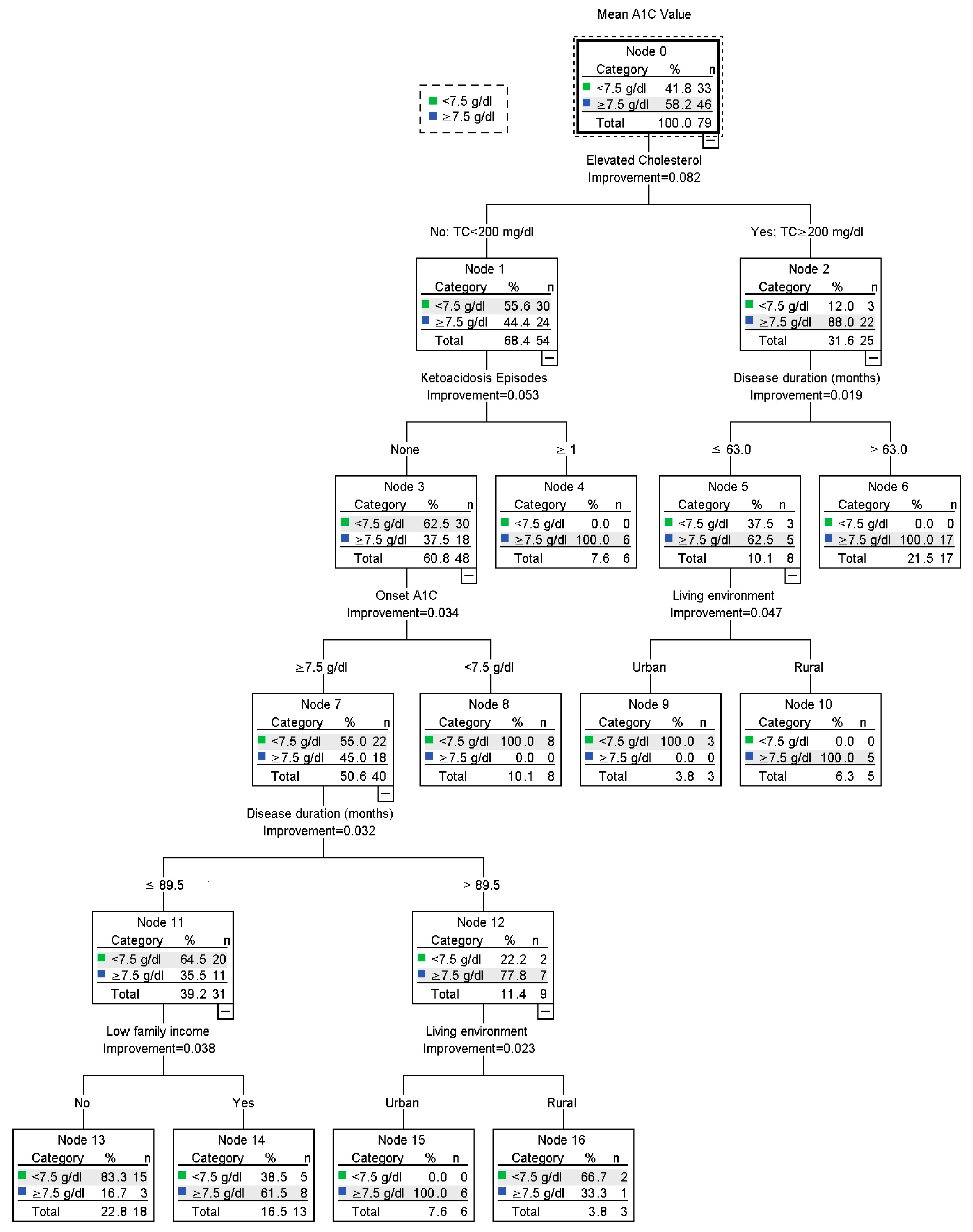
| Risk Category | Poor Glycemic Control (%) | Subgroup Characteristics |
|---|---|---|
| High | 100% | 22 patients with high cholesterol, 17 with a disease duration above 63 months, and 6 with a disease duration under 63 months but living in a rural environment. |
| 12 patients with normal cholesterol, 6 of which presented at least one episode of ketoacidosis (excluding onset) and 6 of which did not present any episodes of ketoacidosis but had an onset A1C above 7.5 g/dL, a disease duration above 89.5 months and lived in an urban environment. | ||
| Moderate | 61.5% | 13 patients with normal cholesterol levels, no ketoacidosis episodes, an A1C onset above 7.5 g/dL, a disease duration under 89.5 months, and a low family income. |
| 33.3% | 3 patients with normal cholesterol levels, no ketoacidosis episodes, an onset of A1C above 7.5 g/dL, and disease duration above 89.5 months, originating from a rural environment. | |
| Low | 16.7% | 18 patients with normal cholesterol levels, average or high family income, a disease duration of 89.5 months or under, an onset A1C of 7.5 g/dL or under, and no ketoacidosis episodes. |
| 0% | 8 patients with normal cholesterol levels, no ketoacidosis episodes, and an onset A1C of 7.5 g/dL or under. | |
| 0% | 3 patients with high cholesterol levels had a disease duration of 63 months or less and lived in an urban environment. |
| High Risk | Medium Risk | Low Risk | ||||||||
|---|---|---|---|---|---|---|---|---|---|---|
| Node 4 | Node 6 | Node 10 | Node 15 | Node 14 | Node 16 | Node 13 | Node 8 | Node 9 | ||
| High risk | Cluster 1 | 6 (100%) | 9 (52.9%) | 2 (40%) | 1 (16.7%) | 1 (7.7%) | 0 (0%) | 0 (0%) | 0 (0%) | 0 (0%) |
| Moderate risk | Cluster 2 | 0 (0%) | 4 (23.5%) | 3 (60%) | 0 (0%) | 5 (38.5%) | 3 (100%) | 2 (11.1%) | 2 (25%) | 0 (0%) |
| Cluster 3 | 0 (0%) | 2 (11.8%) | 0 (0%) | 4 (66.7%) | 7 (53.8%) | 0 (0%) | 9 (50%) | 5 (62.5%) | 1 (33%) | |
| Low risk | Cluster 4 | 0 (0%) | 0 (0%) | 0 (0%) | 1 (16.7%) | 0 (0%) | 0 (0%) | 7 (38.9%) | 1 (12.5%) | 2 (66%) |
| Variable | Method | Key Findings | Clinical Implications |
|---|---|---|---|
| Ketoacidosis episodes | Binary logistic regression | Highest impact variable in binary logistics regression. Essential predictor is prevalent across all methods. Steep modulatory impact across the conglomeration of all other predictor categories in CART and two-step cluster analysis. | High impact predictor. Requires attentive management and assertive prevention. |
| Two-step cluster analysis | |||
| CART | |||
| Family Income | Binary logistic regression | Essential predictor is prevalent across all methods. | An integrative approach is necessary to handle the environmental conditions of pediatric patients with type 1 diabetes. In particular, interventions should be adapted to caretaker comprehension levels and available resources with tailored information and management strategies for each category. |
| Two-step cluster analysis | |||
| CART | |||
| Living environment | Two-step cluster analysis | Important predictor, prevalent across methods that employ patient categorization | |
| CART | |||
| Higher maternal education | Two-step cluster analysis | Important modulatory effect when taken in conjunction with other essential socioeconomic and disease-related characteristics | |
| A1C at onset | Binary logistics regression | Prevalent across prediction algorithms | Disease onset can predict future outcomes. More aggressive screening strategies may be warranted. |
| CART | |||
| Elevated Cholesterol | Binary logistics regression | Prevalent across prediction algorithms | An integrated approach to lifestyle management and risk factor mitigation is essential. While some predictors may have a smaller impact on glycemic control, their modifiable nature presents unique therapeutic opportunities for an overall increased effect on clinical outcomes. |
| CART | |||
| Elevated Triglycerides | Two-step cluster analysis | Modulatory effect in conjunction with other disease characteristics and socioeconomic status | |
| BMI Z-score | Binary logistics regression | Low impact predictor, but present nonetheless | |
| Disease duration | CART | Modulatory impact on disease profiles | Dynamic changes within the disease patterns require attentive monitoring of pediatric patients with type 1 diabetes. Treatment up-scaling may take this aspect into consideration. |
Disclaimer/Publisher’s Note: The statements, opinions and data contained in all publications are solely those of the individual author(s) and contributor(s) and not of MDPI and/or the editor(s). MDPI and/or the editor(s) disclaim responsibility for any injury to people or property resulting from any ideas, methods, instructions or products referred to in the content. |
© 2023 by the authors. Licensee MDPI, Basel, Switzerland. This article is an open access article distributed under the terms and conditions of the Creative Commons Attribution (CC BY) license (https://creativecommons.org/licenses/by/4.0/).
Share and Cite
Neamtu, B.; Negrea, M.O.; Neagu, I. Predicting Glycemic Control in a Small Cohort of Children with Type 1 Diabetes Using Machine Learning Algorithms. Mathematics 2023, 11, 4388. https://doi.org/10.3390/math11204388
Neamtu B, Negrea MO, Neagu I. Predicting Glycemic Control in a Small Cohort of Children with Type 1 Diabetes Using Machine Learning Algorithms. Mathematics. 2023; 11(20):4388. https://doi.org/10.3390/math11204388
Chicago/Turabian StyleNeamtu, Bogdan, Mihai Octavian Negrea, and Iuliana Neagu. 2023. "Predicting Glycemic Control in a Small Cohort of Children with Type 1 Diabetes Using Machine Learning Algorithms" Mathematics 11, no. 20: 4388. https://doi.org/10.3390/math11204388
APA StyleNeamtu, B., Negrea, M. O., & Neagu, I. (2023). Predicting Glycemic Control in a Small Cohort of Children with Type 1 Diabetes Using Machine Learning Algorithms. Mathematics, 11(20), 4388. https://doi.org/10.3390/math11204388