Nonparametric Estimation of Multivariate Copula Using Empirical Bayes Methods

Abstract

In the fields of finance, insurance, system reliability, etc., it is often of interest to measure the dependence among variables by modeling a multivariate distribution using a copula. The copula models with parametric assumptions are easy to estimate but can be highly biased when such assumptions are false, while the empirical copulas are nonsmooth and often not genuine copulas, making the inference about dependence challenging in practice. As a compromise, the empirical Bernstein copula provides a smooth estimator, but the estimation of tuning parameters remains elusive. The proposed empirical checkerboard copula within a hierarchical empirical Bayes model alleviates the aforementioned issues and provides a smooth estimator based on multivariate Bernstein polynomials that itself is shown to be a genuine copula. Additionally, the proposed copula estimator is shown to provide a more accurate estimate of several multivariate dependence measures. Both theoretical asymptotic properties and finite-sample performances of the proposed estimator based on simulated data are presented and compared with some nonparametric estimators. An application to portfolio risk management is included based on stock prices data.

1. Introduction

Copula models are useful tools for the analysis of multivariate data, since by using the well-known Sklar’s theorem, any multivariate joint distribution can be decomposed into its univariate marginal distributions and a copula function, which allows capturing of the arbitrary dependence structure between several random variables. As a result, copulas have been widely used in the fields of finance, insurance, system reliability, etc., among many other application areas. See, e.g., Jaworski et al. [1], Joe [2] and Nelsen [3] for more details about copulas and their applications.

Given a random vector $(X_1,\dots ,X_d)$ with joint cumulative distribution function (CDF) F and continuous marginal CDFs $F_j,j\in \{1,\cdots ,d\}$, by Sklar’s theorem (Sklar [4]), the CDF F can be expressed uniquely as $F(x_1,\dots ,x_d)=C(F_1\left(x_1\right),\dots ,F_d\left(x_d\right))$, where $C(·)$ denotes the copula function. A copula is itself the joint CDF of a random vector $(U_1=F_1\left(X_1\right),\dots ,U_d=F_d\left(X_d\right))$ having its marginals as uniform distributions on $[0,1]$, henceforth denoted by $Unif[0,1]$. It is to be noted that the original results in Sklar [4] are also applicable to discrete-valued random variables; however, the focus of this paper is modeling continuous-valued multivariate random vectors. Thus, for the rest of the paper, we assume that the marginal CDFs $F_j,j\in \{1,\cdots ,d\}$ are absolutely continuous.

As a copula plays an important role in capturing the general dependence structure between multiple variables, it is critical to estimate copulas in an accurate way, especially in higher dimensions where the dependence structure becomes much more complicated, is often illusive, and may even be supported on a lower-dimensional manifold. One of the primary goals of this paper is to estimate a smooth copula function C from a random sample of n independent identically distributed (iid) observations $(X_{i1},\dots ,X_{id})\stackrel{iid}{\sim }F(x_1,\dots ,x_d)$ for $i\in \{1,\dots ,n\}$.

Many parametric families have been proposed for modeling multivariate copulas, and there has been previous work addressing the corresponding parametric estimation methods. For detailed discussions, see, e.g., Joe [5], Joe [2], McNeil et al. [6], Nelsen [3], Smith [7] and Žežula [8], etc. However, regardless of how sophisticated and flexible the parametric models are that we may use, they might still lead to biased copula estimates when the parametric model is misspecified and thus may not be able to capture complex dependence structures required in practice. Compared to standard multivariate copulas, vine copula models allow for more flexibility in capturing complex dependency structures using appropriate vine tree structures by choosing bivariate copula families for each node of pair copulas from a vast array of parametric bivariate copulas. But it is often challenging to obtain estimates of multivariate dependence measures that involve high-dimensional integrals which are often algebraically intractable by using vine copulas.

Thus, recognizing some of the abovementioned limitations of parametric copula models, a variety of nonparametric estimators have been proposed for multivariate copula estimation. Most of the available nonparametric estimators rely on the empirical methods, e.g., the empirical copula and its multilinear extension, the empirical multilinear copula (Deheuvels [9]; Fermanian et al. [10]; Genest et al. [11]), or kernel-based methods such as local linear estimator (Chen and Huang [12]), mirror reflection estimator (Gijbels and Mielniczuk [13]), and improvements of these two estimators (Omelka et al. [14]). See alsoRémillard and Scaillet [15] and Scaillet and Fermanian [16] for other nonparametric copula estimators. However, except for the empirical multilinear copula, most of these estimators are valid copulas only asymptotically, meaning that they are not necessarily genuine copulas for finite samples. Moreover, multivariate dependent measures (e.g., Spearman’s rho, Kendall’s tau, etc.) based on such estimated copulas could take values outside of their natural range, thus making them unattractive in practice. On the other hand, there has been recent work on Bayesian nonparametric methods for estimating general d-dimensional copulas and, among many others, a noteworthy Bayesian nonparametric model is based on an infinite mixture of multivariate Gaussian or the skew-normal copulas proposed by Wu et al. [17]. The infinite mixture models provide a lot of flexibility in modeling various dependence structures, but those typically lack simple (analytic) expressions of dependence measures making them harder to compute in practice.

The primary focus of this paper is the nonparametric estimation of multivariate copulas for any arbitrary dimensions that are genuine copulas for any finite sample size and are uniformly consistent as the sample size becomes large. We consider an extension of the Bernstein copula (Sancetta and Satchell [18]), which is a family of copulas defined in terms of multivariate Bernstein polynomials. One of the primary advantages of the Bernstein copula is that it provides a class of nested models that are able to uniformly approximate any multivariate copula with minimal regularity conditions. A simple case of the Bernstein copula is the empirical Bernstein copula, which is a nonparametric copula estimator proposed by Sancetta and Satchell [18]. The asymptotic properties of the empirical Bernstein copula are well studied in Janssen et al. [19], and its application in testing independence is described in Belalia et al. [20]. The application of the Bernstein copula to the modeling of dependence structures of non-life-insurance risks is provided in Diers et al. [21], among many other applications.

However, the empirical Bernstein copula has two main drawbacks that could prevent us from obtaining accurate copula estimation for small samples: (i) the empirical Bernstein copula is not necessarily a valid copula itself, which is a common disadvantage for most nonparametric copula estimators; and (ii) the degrees of Bernstein polynomials are often set to be equal to an integer across different dimensions, which limits the flexibility of the Bernstein copula and thus might not be appropriate for large dimensions.

In order to address the above-described problem (i), Segers et al. [22] showed that the empirical Bernstein copula is a genuine copula if and only if all the polynomial degrees are divisors of the sample size, and further proposed a new copula estimator called the empirical beta copula, which can be seen as a special case of the empirical Bernstein copula when the degrees of Bernstein polynomials are all set equal to the sample size. The empirical beta copula is a valid copula itself and has been shown to outperform some classical copula estimators in terms of bias and variance, but it always has a larger variance compared to the empirical Bernstein copula with smaller polynomial degrees. It is surprising that much less attention has been given to the problem (ii), and even for equally set degrees, there has been limited work on the data-dependent choice of degrees in the literature. Janssen et al. [19] recommended an optimal choice of the equal degrees in the bivariate case by minimizing the asymptotic mean squared error. Nevertheless, such a choice requires the knowledge of the first- and second-order partial derivatives, which might not be easy to estimate in practice. Burda and Prokhorov [23] put priors on the polynomial degrees; however, their priors did not rely on data or sample size, and they used multivariate Bernstein density instead of Bernstein copula density. The Dirichlet process assigned as the prior for the copula does not guarantee the copula estimate to be a valid copula itself. In addition, the number of weights grows exponentially as the dimension increases, leading to computational inefficiency of MCMC methods for larger dimensions. To the best of our knowledge, Lu and Ghosh [24] first developed a data-dependent grid search algorithm for the selection of polynomial degrees, which has shown superior empirical estimation properties for small- to moderate-sized samples, but the methodology is limited to bivariate cases, and extension to larger dimensions remains challenging.

For the purpose of addressing the two problems described above, we introduce a new nonparametric smooth estimator for multivariate copula that we call the empirical checkerboard Bernstein copula (ECBC), which is constructed by extending the Bernstein copula, allowing for varying degrees of the polynomials. It is shown to be a genuine smooth copula for any number of degrees and any finite sample size. Furthermore, we develop an empirical Bayesian method that takes the data into account to automatically choose the degrees of the proposed estimator using its posterior distribution, thereby accounting for the uncertainty of such tuning parameter selection. As shown in Segers et al. [22], larger degrees of the Bernstein copula lead to a larger variance of the estimation, so a choice of degrees that is relatively small compared to the sample size but sufficient for a good copula estimation is desirable. The degrees are allowed to be dimension-varying within the Bayesian model, which provides much more flexibility and accuracy, especially in higher dimensions.

It is especially noteworthy that while the focus of the paper is to estimate the copula function, it is straightforward to obtain a closed-form estimate of the corresponding copula density by taking derivatives of the ECBC. However, direct estimation of a closed-form copula function has many advantages compared to first estimating a copula density, e.g., it is often easier to differentiate than to integrate for higher dimensions. In addition, for those copulas which are not absolutely continuous, such as Marshall–Olkin copulas (Embrechts et al. [25]) having support on a possibly lower-dimensional manifold, the direct estimation of the copula density could be difficult. Owing to the closed form of the estimated copula function and its density, it can be shown that the proposed ECBC allows for straightforward estimation of various dependence measures.

The rest of the paper is organized as follows: in Section 2, we present an empirical Bayes nonparametric copula model. In Section 2.1, we derive the closed-form expression of estimates of popular multivariate dependence measures based on the novel methodology of multivariate copula estimation. We then illustrate the performance of the proposed methodology in Section 3. Section 3.1 shows the finite-sample performance for bivariate cases. The accuracy of the estimation of multivariate dependence measures is investigated in Section 3.2. Section 3.3 illustrates the estimation of tuning parameters of the proposed ECBC copula estimator, and the comparison with the empirical Bernstein copulas is provided in Section 3.4. Section 4 provides an application to portfolio risk management. Finally, we make some general comments in Section 5.

2. An Empirical Bayes Nonparametric Copula Model

Suppose we have i.i.d. samples $(X_{i1},\dots ,X_{id})\sim F(x_1,\dots ,x_d),i\in \{1,\dots ,n\}$, where F is a cumulative distribution function and $F_j$ is the absolutely continuous marginal CDF of the j-th component. By Sklar ’s theorem (Sklar [4]), there exists a unique copula $C(·)$ such that

$$F(x_1,\dots ,x_d)=C(F_1\left(x_1\right),\dots ,F_d\left(x_d\right)),\forall (x_1,\dots ,x_d)\in {\mathbb{R}}^d,$$

and

$$(F_1\left(X_1\right),\dots ,F_d\left(X_d\right))\sim C.$$

The Bernstein copula is a family of copulas defined in terms of Bernstein polynomials, and it was first introduced by Sancetta and Satchell [18]. It is a flexible model that can be used to uniformly approximate any copula. The Bernstein polynomial with degrees $(m_1,\dots ,m_d)$ of a function $C:{[0,1]}^d\to \mathbb{R}$ is defined as

$$B_m\left(C\right)\left(\mathbf{u}\right)=\sum _{k_1=0}^{m_1}\cdots \sum _{k_d=0}^{m_d}C\left(\frac{k_1}{m_1},\dots ,\frac{k_d}{m_d}\right)\prod _{j=1}^d\left(\genfrac{}{}{0pt}{}{m_j}{k_j}\right)u_j^{k_j}{(1-u_j)}^{m_j-k_j},$$

(1)

and $B_m\left(C\right)$ is called the Bernstein copula when C is a copula.

A general estimation for the Bernstein copula of an unknown copula hlC is the empirical Bernstein copula (Sancetta and Satchell [18]) $B_m\left(C_n\right)$, where $C_n$ is the rank-based empirical copula. We denote the empirical Bernstein copula as

$$C_{m,n}\left(\mathbf{u}\right)=\sum _{k_1=0}^{m_1}\cdots \sum _{k_d=0}^{m_d}{\widehat{\theta }}_{k_1,\dots ,k_d}\prod _{j=1}^d\left(\genfrac{}{}{0pt}{}{m_j}{k_j}\right)u_j^{k_j}{(1-u_j)}^{m_j-k_j},$$

where

$${\widehat{\theta }}_{k_1,\dots ,k_d}=C_n\left(\frac{k_1}{m_1},\dots ,\frac{k_d}{m_d}\right)=\frac{1}{n}\sum _{i=1}^n\prod _{j=1}^d\mathbb{I}\left(F_{nj}^{\ast }\left(X_{ij}\right)\le \frac{k_j}{m_j}\right).$$

where $\mathbb{I}(·)$ denotes indicator function, and slightly modified empirical marginal distribution functions are defined as

$$F_{nj}^{\ast }\left(x_j\right)=\frac{1}{n+1}\sum _{i=1}^n\mathbb{I}(X_{ij}\le x_j),\mathrm{for}j\in \{1,\cdots ,d\},$$

where the modification $1/(n+1)$ instead of $1/n$ modifies the standard empirical marginal distribution to be away from 1 in order to reduce potential problems at boundaries.

However, the empirical Bernstein copula $C_{m,n}$ is not guaranteed to be a valid copula for finite samples as the empirical copula $C_n$ is not necessarily a genuine copula. Segers et al. [22] showed that the empirical Bernstein copula $C_{m,n}$ is a copula if and only if all the degrees $m_1,...,m_d$ are divisors of n. In order to obtain a valid copula estimation for any degrees, we replace the empirical copula $C_n$ with the empirical checkerboard copula $C_n^{\#}$, which is a simple multilinear extension of the empirical copula defined as

$$C_n^{\#}\left(\mathbf{u}\right)=\frac{1}{n}\sum _{i=1}^n\prod _{j=1}^{d}min(max((n{u}_j-R_{i,j}^{\left(n\right)}+1),0),1),$$

where $R_{i,j}^{\left(n\right)}$ is the rank of $X_{ij}$ among $X_{1j},\dots ,X_{nj}$; see, e.g., Carley and Taylor [26] and Li et al. [27] for more details. Notice that the main difference between the empirical copula $C_n$ and the empirical checkerboard copula $C_n^{\#}$ is that $C_n^{\#}$ is a genuine copula, so we can obtain a valid copula estimation $C_{m,n}^{\#}$ taking the form

$$C_{m,n}^{\#}\left(\mathbf{u}\right)=\sum _{k_1=0}^{m_1}\cdots \sum _{k_d=0}^{m_d}{\tilde{\theta }}_{k_1,\dots ,k_d}\prod _{j=1}^d\left(\genfrac{}{}{0pt}{}{m_j}{k_j}\right)u_j^{k_j}{(1-u_j)}^{m_j-k_j},$$

(2)

where

$${\tilde{\theta }}_{k_1,\dots ,k_d}=C_n^{\#}\left(\frac{k_1}{m_1},\dots ,\frac{k_d}{m_d}\right)=\frac{1}{n}\sum _{i=1}^n\prod _{j=1}^{d}min(max\left(\left(n\frac{k_j}{m_j}-R_{i,j}^{\left(n\right)}+1\right),0),1\right),$$

(3)

and we call the proposed empirical checkerboard Bernstein copula (ECBC).

Unlike the empirical Bernstein copula, the ECBC is a genuine copula for any degrees $m_1,m_2,\dots ,m_d\in {\mathbb{Z}}^{+}$, and any fixed sample size n. It is known that Bernstein polynomials with smaller values of degrees $m_j$s may lead to biased estimates while unnecessary larger degrees of Bernstein polynomials will necessarily lead to larger variances. Therefore, it is critical to choose the proper degrees of the ECBC based on a given sample. In order to do that, we develop an empirical Bayes method for choosing ‘optimal’ degrees $(m_1,m_2,\dots ,m_d)$, where $m_j$s are allowed to be different for different $j\in \{1,\cdots ,d\}$ and also depend on the random sample of observations.

As illustrated in Sancetta and Satchell [18], using partial derivatives of (2) with respect to each $u_j$ and rearranging, we can obtain the density corresponding to ECBC as follows:

$$\begin{array}{cc}\hfill c_{m,n}^{\#}\left(\mathbf{u}\right)& =\sum _{k_1=0}^{m_1-1}\cdots \sum _{k_d=0}^{m_d-1}{\tilde{w}}_{k_1,\dots ,k_d}\prod _{j=1}^d{m}_j\left(\genfrac{}{}{0pt}{}{m_j-1}{k_j}\right)u_j^{k_j}{(1-u_j)}^{m_j-k_j-1}\hfill \\ \hfill & =\sum _{k_1=0}^{m_1-1}\cdots \sum _{k_d=0}^{m_d-1}{\tilde{w}}_{k_1,\dots ,k_d}\prod _{j=1}^{d}Beta(u_j,k_j+1,m_j-k_j),\hfill \end{array}$$

(4)

where

$$\begin{array}{cc}\hfill {\tilde{w}}_{k_1,\dots ,k_d}& =\sum _{l_1=0}^1\cdots \sum _{l_d=0}^1{(-1)}^{d+l_1+\dots +l_d}{C}_n^{\#}\left(\frac{k_1+l_1}{m_1},\dots ,\frac{k_d+l_d}{m_d}\right).\hfill \\ \hfill \end{array}$$

(5)

Clearly, the Bernstein copula is a mixture of independent Beta distributions leading to a tensor product form. For notational convenience, let us denote

$$U_{ij}\equiv F_{nj}^{\ast }\left(X_{ij}\right)i\in \{1,\dots ,n\},j\in \{1,\cdots ,d\},$$

Following the work by Gijbels et al. [28], the pseudo-observations $(U_{i1},\dots U_{id}),i\in \{1,\dots ,n\}$ can be treated as samples from $(F_1\left(U_{i1}\right),\dots ,F_d\left(U_{id}\right))\sim C$. We then use this approximation to build an empirical Bayesian hierarchical model:

$$U_{ij}|L_{ij}\stackrel{ind}{\sim }Beta(L_{ij}+1,m_j-L_{ij}),i\in \{1,\dots ,n\},j\in \{1,\cdots ,d\},$$

$$L_{ij}=\lfloor m_j{V}_{ij}\rfloor ,$$

where $\lfloor a\rfloor$ is the ‘floor’ function denoting the largest integer not exceeding the value a, and

$$(V_{i1},\dots ,V_{id})\stackrel{i.i.d}{\sim }{C}_n^{\#}(·),i\in \{1,\dots ,n\},$$

i.e., $(V_{i1},\dots ,V_{id}),i\in \{1,\dots ,n\}$ are samples from the empirical checkerboard copula $C_n^{\#}$. It then follows that

$$\begin{array}{cc}\hfill {\tilde{w}}_{k_1,\dots ,k_d}& =Pr(L_{i1}=k_1,\dots ,L_{id}=k_d)\hfill \\ \hfill & =Pr\left(\frac{k_1}{m_1}\le V_{i1}<\frac{k_1+1}{m_1},\dots ,\frac{k_d}{m_d}\le V_{id}<\frac{k_d+1}{m_d}\right).\hfill \end{array}$$

Based on the proposition 1 in Genest et al. [11], $V_{ij}$ can be drawn using the following hierarchical scheme:

$$\begin{array}{c}\hfill {\pi }_i\stackrel{i.i.d}{\sim }DisUnif\{1,\dots ,n\},i\in \{1,\dots ,n\},\\ \hfill {\Lambda }_{ij}\stackrel{i.i.d}{\sim }Unif(0,1)i\in \{1,\dots ,n\},j\in \{1,\cdots ,d\}.\\ \hfill V_{ij}=(1-{\Lambda }_{ij})F_{n,j}(X_{{\pi }_{i}j}-)+{\Lambda }_{ij}{F}_{n,j}\left(X_{{\pi }_{i}j}\right),\end{array}$$

where $F_{n,j}\left(x_j\right)=1/n{\sum }_{i=1}^{n}I(X_{ij}\le x_j)$ and $DisUnif$ denotes the discrete uniform distribution, i.e., $Pr[{\pi }_i=j]=1/n$ for $j\in \{1,\cdots ,d\}$. Assuming that there are no ties in the pseudo samples $U_{1j},\dots ,U_{nj}$ (owing to absolute continuity of marginal distributions or breaking it by random assignment in practice), we can equivalently represent the $V_{ij}$’s more conveniently as

$$\begin{array}{cc}\hfill V_{ij}& =(1-{\Lambda }_{ij})\frac{R_{{\pi }_i,j}^{\left(n\right)}-1}{n}+{\Lambda }_{ij}\frac{R_{{\pi }_i,j}^{\left(n\right)}}{n}\hfill \\ \hfill & =\frac{R_{{\pi }_i,j}^{\left(n\right)}-1+{\Lambda }_{ij}}{n}.\hfill \end{array}$$

Next, to account for the uncertainty in the estimation of the degrees $m_j$s, we propose to introduce a sample-size-dependent empirical prior distribution on the degrees $m_1,\dots ,m_d$ and obtain posterior estimates by Markov chain Monte Carlo (MCMC) methods. This would not only allow for the almost automatic adaptive estimation of the degrees (based on the observed data) but would also allow for quantifying the uncertainty of this crucial tuning parameter vector. Notice that the idea of putting priors on the polynomial degrees was also adopted by Burda and Prokhorov [23]. However, their priors did not rely on data or sample size and they used multivariate Bernstein density instead of Bernstein copula density, i.e., the weights belonged to a simplex without any more constraints. A Dirichlet process with a baseline of uniform distribution on ${[0,1]}^d$ was assigned as the prior for the copula C in (1), which did not guarantee C to be a valid copula. In order to avoid the construction of priors under constraints, we use the empirical estimates for the coefficients of the Bernstein copula instead of assigning priors to them.

Motivated by the asymptotic theory of the empirical Bernstein estimator, e.g., as in Janssen et al. [29], we propose the hierarchical shifted Poisson distributions as the prior distribution for $m_1,\dots m_d$:

$$m_j\mid {\alpha }_j\stackrel{ind}{\sim }Poisson\left(n^{{\alpha }_j}\right)+1,j\in \{1,\cdots ,d\}.$$

(6)

and

$${\alpha }_j\stackrel{i.i.d}{\sim }Unif\left(\frac{1}{3},\frac{2}{3}\right),j\in \{1,\cdots ,d\}.$$

(7)

The following theorem provides the large-sample consistency of the ECBC using the same set of assumptions as required for the large-sample consistency of the empirical checkerboard copula.

Theorem 1.

Given the empirical priors distribution of $m_1,\dots ,m_d$ as in (6) and (7), and assuming the regularity conditions for the consistency of the empirical checkerboard copula, the proposed ECBC is consistent in the following sense:

$$E\left(\right||C_{m,n}^{\#}-C\left|\right|)=E\left[\underset{\mathbf{u}\in {[0,1]}^d}{sup}\left|C_{m,n}^{\#}\left(\mathbf{u}\right)-C\left(\mathbf{u}\right)\right|\right]\stackrel{a.s.}{\to }0\mathit{as}n\to \infty .$$

where the expectation is taken with respect to the empirical prior distribution.

Proof. 

We denote the ECBC as $B_m\left(C_n^{\#}\right)$ for simplicity. Also, the empirical Bernstein copula and the Bernstein copula are denoted as $B_m\left(C_n\right)$ and $B_m\left(C\right)$, respectively. Let ${\displaystyle \left|\right|g\left|\right|=\underset{\mathbf{u}\in {[0,1]}^d}{sup}g\left(\mathbf{u}\right)}$ denote the supremum norm of a function $g(·)$ defined on d-dimensional square ${[0,1]}^d$. Using the familiar triangle inequality, we have

$$\left|\right|B_m\left(C_n^{\#}\right)-C\left|\right|\le \left|\right|B_m\left(C_n^{\#}\right)-B_m\left(C_n\right)\left|\right|+\left|\right|B_m\left(C_n\right)-B_m\left(C\right)\left|\right|+\left|\right|B_m\left(C\right)-C\left|\right|$$

First, under the assumption that the marginal CDFs are continuous, it follows from Remark 2 in Genest et al. [11] that

$$\left|\right|C_n^{\#}-C_n\left|\right|\le \frac{d}{n}.$$

Next, notice that

$$\begin{array}{cc}\hfill & \left|\right|B_m\left(C_n^{\#}\right)-B_m\left(C_n\right)\left|\right|\hfill \\ \hfill & =\underset{\mathbf{u}\in {[0,1]}^d}{sup}\left|\sum _{k_1=0}^{m_1}\cdots \sum _{k_d=0}^{m_d}\left(C_n^{\#}\left(\frac{k_1}{m_1},\dots ,\frac{k_d}{m_d}\right)-C_n\left(\frac{k_1}{m_1},\dots ,\frac{k_d}{m_d}\right)\right)\prod _{j=1}^d\left(\genfrac{}{}{0pt}{}{m_j}{k_j}\right)u_j^{k_j}{(1-u_j)}^{m_j-k_j}\right|\hfill \\ \hfill & \le \underset{0\le k_1\le m_1,\dots 0\le k_d\le m_d}{max}\left|C_n^{\#}\left(\frac{k_1}{m_1},\dots ,\frac{k_d}{m_d}\right)-C_n\left(\frac{k_1}{m_1},\dots ,\frac{k_d}{m_d}\right)\right|\hfill \\ \hfill & \le \left|\right|C_n^{\#}-C_n\left|\right|\le \frac{d}{n}\hfill \end{array}$$

In the above, the second inequality follows from the fact that since $\left(\genfrac{}{}{0pt}{}{m_j}{k_j}\right)u_j^{k_j}{(1-u_j)}^{m_j-k_j},k_j\in \{0,\dots ,m_j\}$ are binomial probabilities, ${\sum }_{k_j=0}^{m_j}\left(\genfrac{}{}{0pt}{}{m_j}{k_j}\right)u_j^{k_j}{(1-u_j)}^{m_j-k_j}=1$ for any $u_j\in [0,1]$ and for any $j\in \{1,\cdots ,d\}$.

Next, by using Lemma 1 in Janssen et al. [19] and Equation (3) in Kiriliouk et al. [30], we obtain

$$\begin{array}{cc}\hfill \left|\right|C_n-C\left|\right|& \le \left|\right|C_n-F_n(F_{n1}^{-1}\left(u_1\right),\dots ,F_{nd}^{-1}\left(u_d\right))\left|\right|\hfill \\ & +\left|\right|F_n(F_{n1}^{-1}\left(u_1\right),\dots ,F_{nd}^{-1}\left(u_d\right))-F(F_1^{-1}\left(u_1\right),\dots ,F_d^{-1}d\left(u_d\right)\left|\right|\hfill \\ & \le \frac{d}{n}+O\left(n^{-1/2}{(lnlnn)}^{1/2}\right)a.s.\hfill \\ \hfill & =O\left(n^{-1/2}{(lnlnn)}^{1/2}\right)a.s..\hfill \end{array}$$

Hence, it now follows that

$$\left|\right|B_m\left(C_n\right)-B_m\left(C\right)\left|\right|\le \left|\right|C_n-C\left|\right|\le O\left(n^{-1/2}{(lnlnn)}^{1/2}\right),a.s.$$

Also, by using Lemma 3.2 in Segers et al. [22], we have

$$\left|\right|B_m\left(C\right)-C\left|\right|\le \sum _{j=1}^d\frac{1}{2\sqrt{m_j}}$$

Thus, combining the above inequalities that are satisfied almost surely (a.s.) for every fixed $m_j$s, we obtain

$$\begin{array}{cc}\hfill \left|\right|B_m\left(C_n^{\#}\right)-C\left|\right|& \le \left|\right|B_m\left(C_n^{\#}\right)-B_m\left(C_n\right)\left|\right|+\left|\right|B_m\left(C_n\right)-B_m\left(C\right)\left|\right|+\left|\right|B_m\left(C\right)-C\left|\right|\hfill \\ \hfill & \le \frac{d}{n}+\sum _{j=1}^d\frac{1}{2\sqrt{m_j}}+O\left(n^{-1/2}{(lnlnn)}^{1/2}\right)a.s.\hfill \end{array}$$

Next, we consider the proposed empirical priors on the degrees $m_1,\dots ,m_d$ to be

$$m_j|{\alpha }_j\stackrel{ind}{\sim }Poisson\left(n^{{\alpha }_j}\right)+1\mathrm{and}{\alpha }_j\stackrel{iid}{\sim }Unif\left(\frac{1}{3},\frac{2}{3}\right)\mathrm{for}j\in \{1,\cdots ,d\}.$$

   □

We make use of the following simple lemma:

Lemma 1.

Suppose $M\sim Poisson\left(\lambda \right)$, then $E\left[\frac{1}{\sqrt{M+1}}\right]\le \sqrt{\frac{1-e^{-\lambda }}{\lambda }}$.

Proof of Lemma 1.

By Jensen’s inequality for the square-root function, it follows that

$$E\left(\frac{1}{\sqrt{M+1}}\right)\le \sqrt{E\left(\frac{1}{M+1}\right)}=\sqrt{\frac{1}{\lambda }\sum _{m=0}^{\infty }\frac{{\lambda }^{m+1}{e}^{-\lambda }}{(m+1)!}}=\sqrt{\frac{1-e^{-\lambda }}{\lambda }}.$$

Notice that as ${\alpha }_j\sim Unif(1/3,2/3)$, $Pr({\alpha }_j>1/3)=1$ and conditioning on ${\alpha }_j$, we then have, by the above lemma, $E\left(\sqrt{1/m_j}|{\alpha }_j\right)\le \sqrt{(1-e^{-n^{{\alpha }_j}})/n^{{\alpha }_j}}\to 0$ as $n\to \infty$. Thus, taking expectation with respect to the prior distribution, it follows that

$$\begin{array}{cc}\hfill E\left|\right|B_m\left(C_n^{\#}\right)-C\left|\right|& \le E\left|\right|B_m\left(C_n^{\#}\right)-B_m\left(C_n\right)\left|\right|+E\left|\right|B_m\left(C_n\right)-B_m\left(C\right)\left|\right|+E\left|\right|B_m\left(C\right)-C\left|\right|\hfill \\ \hfill & \le \frac{d}{n}+\sum _{j=1}^d\frac{1}{2}E\left(\frac{1}{\sqrt{m_j}}\right)+O\left(n^{-1/2}{(lnlnn)}^{1/2}\right)\to 0asn\to \infty a.s.\hfill \end{array}$$

   □

Notice that in the above result, the a.s. convergence is with respect to the empirical marginal distribution of the data integrating out the conditional empirical distribution of data (given the $m_j$s) weighted by the empirical prior distribution of the tuning parameters $m_j$s. This is not the usual notion of posterior consistency, but, rather, the notion can be viewed as using an integrated likelihood approach (Berger et al. [31]) with respect to the empirical marginal distribution obtained by integrating the priors given by Equations (6) and (7).

It is to be noted that the joint posterior distribution of ($m_1,\dots m_d$) may not necessarily preserve an exchangeable structure as the above prior. Using the empirical Bayes hierarchical structure of the above-proposed model, it can be shown that efficient MCMC methods can be utilized to draw approximate samples from the path of a geometrically ergodic Markov Chain with posterior distribution as its stationary distribution. By generating a sufficiently large number of MCMC samples, we can estimate the marginal posterior mode of the discrete-valued parameter $m_j$s as final estimates. Let $m_{j1},\dots ,m_{jK}$ denote K MCMC samples of $m_j,j\in \{1,\cdots ,d\}$ and for each j, let ${\tilde{m}}_{j1}<{\tilde{m}}_{j2}<\cdots <{\tilde{m}}_{j{D}_j}$ denote the distinct values among these MCMC samples. Then, the (marginal) posterior mode of $m_j$ is estimated by

$${\widehat{m}}_j=\underset{m_{jb},b=1,\dots ,D_j}{\mathrm{argmax}}\sum _{a=1}^K\mathbb{I}(m_{ja}={\tilde{m}}_{jb}),j\in \{1,\cdots ,d\}.$$

The final estimate of the smooth copula based on the proposed ECBC is then given by

$$C_{\widehat{m},n}^{\#}\left(\mathbf{u}\right)=\sum _{k_1=0}^{{\widehat{m}}_1}\cdots \sum _{k_d=0}^{{\widehat{m}}_d}{\tilde{\theta }}_{k_1,\dots ,k_d}\prod _{j=1}^d\left(\genfrac{}{}{0pt}{}{{\widehat{m}}_j}{k_j}\right)u_j^{k_j}{(1-u_j)}^{{\widehat{m}}_j-k_j}$$

where

$${\tilde{\theta }}_{k_1,\dots ,k_d}=C_n^{\#}\left(\frac{k_1}{{\widehat{m}}_1},\dots ,\frac{k_d}{{\widehat{m}}_d}\right).$$

It is to be noted that other posterior estimates (e.g., posterior mean when it exists or coordinate-wise posterior median or some version of multivariate posterior median) can also be used, but for simplicity (and the requirement that these posterior estimates of $m_j$s be necessarily integer-valued) we chose to use posterior mode based on the marginal posterior distributions of $m_j$s. Through many numerical illustrations, we show the easy applicability of this choice in various examples.

2.1. Multivariate Dependence Estimation

In higher dimensions, it is often of interest to evaluate the strength of dependence among variables. This is often performed using copulas since most dependence measures can be expressed as a function of copulas. Spearman’s rank correlation coefficient (Spearman’s rho) is one of the most widely used dependence measures. For a bivariate copula C, Spearman’s rho can be written as

$$\rho =12{\int }_0^1{\int }_0^{1}C(u,v)dudv-3=12{\int }_0^1{\int }_0^1(C(u,v)-uv)dudv.$$

A multivariate extension of Spearman’s rho given in Nelsen [32] takes the form

$${\rho }_d=\frac{{\int }_{I^d}C\left(\mathbf{u}\right)d\mathbf{u}-{\int }_{I^d}\Pi \left(\mathbf{u}\right)d\mathbf{u}}{{\int }_{I^d}M\left(\mathbf{u}\right)d\mathbf{u}-{\int }_{I^d}\Pi \left(\mathbf{u}\right)d\mathbf{u}}=\frac{d+1}{2^d-(d+1)}\left(2^d{\int }_{I^d}C\left(\mathbf{u}\right)d\mathbf{u}-1\right).$$

(8)

Compared to vine copulas that rely on pair copulas and complex tree structures, one of the advantages of our copula estimator is that it is straightforward to obtain an estimate of multivariate Spearman’s rho as

$${\widehat{\rho }}_d=\frac{d+1}{2^d-(d+1)}\left(2^d\sum _{k_1=0}^{{\widehat{m}}_1}\cdots \sum _{k_d=0}^{{\widehat{m}}_d}{\tilde{\theta }}_{k_1,\dots ,k_d}\prod _{j=1}^d\left(\genfrac{}{}{0pt}{}{{\widehat{m}}_j}{k_j}\right)B(k_j+1,{\widehat{m}}_j-k_j+1)-1\right).$$

(9)

where B is the beta function.

It can be shown that the multivariate Spearman’s rho is bounded by

$$\frac{2^d-(d+1)!}{d!(2^d-d-1)}\le {\rho }_d\le 1,$$

where the lower bound approaches to zero as dimension increases. Since our copula estimator is a genuine copula, the estimate of multivariate d-dimensional Spearman’s rho ${\widehat{\rho }}_d$ can avoid taking values out of the parameter space, which might be an issue for estimates built on other nonparametric copula estimators, e.g., the empirical copula (see Pérez and Prieto-Alaiz [33]).

Similar to Spearman’s rho, Kendall’s tau is another common dependence measure and has its multivariate version as well, which is given by Nelsen [32] as

$${\tau }_d=\frac{1}{2^{d-1}-1}\left(2^d{\int }_{I^d}C\left(\mathbf{u}\right)dC\left(\mathbf{u}\right)-1\right).$$

(10)

By applying (4) and (5), it is also easy to obtain an estimate of multivariate Kendall’s tau based on our copula estimator as

$$\begin{array}{c}\hfill {\widehat{\tau }}_d=\frac{1}{2^{d-1}-1}(2^d\sum _{k_1=0}^{{\widehat{m}}_1-1}\cdots \sum _{k_d=0}^{{\widehat{m}}_d-1}\sum _{l_1=0}^{{\widehat{m}}_1}\cdots \sum _{l_d=0}^{{\widehat{m}}_d}{\tilde{w}}_{k_1,\dots ,k_d}{\tilde{\theta }}_{l_1,\dots ,l_d}\\ \hfill \prod _{j=1}^d{\widehat{m}}_j\left(\genfrac{}{}{0pt}{}{{\widehat{m}}_j-1}{k_j}\right)\left(\genfrac{}{}{0pt}{}{{\widehat{m}}_j}{l_j}\right)B(k_j+l_j+1,2{\widehat{m}}_j-k_j-l_j)-1).\end{array}$$

Thus, using our proposed ECBC copula, not only are we able to obtain a fully nonparametric estimate of any copula function in closed form (once the tuning parameters $m_j,j\in \{1,\cdots ,d\}$ are estimated by their posterior modes), but we are also able to derive the closed-form expression of estimates of the popular multivariate measures of dependence for any arbitrary dimension $d\ge 2$.

Moreover, although we only illustrate the use of multivariate extensions of Kendall’s tau and Spearman’s rho as possible measures of multivariate dependence, any other multivariate notion of dependence measures that are suitable functionals of the underlying copula can also be computed using our closed-form expression of the ECBC estimator. This is particularly advantageous compared to even some of the flexible yet complicated parametric copula family (e.g., Archimedian, multivariate Gaussian, t, etc.) for which it may require high-dimensional numerical integration to compute multivariate versions of Spearman’s rho as given in (8) and/or Kendall’s tau given in (10). For vine copulas, it is particularly challenging to obtain estimates of these multivariate measures of dependence as such high-dimensional integrals are often algebraically and even numerically intractable, say for dimension $d\ge 5$, whereas for ECBC, even when a new measure of dependence is created as a functional of the copula that may be more complicated than those defined in Equations (8) and (10), we can easily obtain a large number of Monte Carlo (MC) samples from the ECBC and use MC-based approximation to estimate such new measures of multivariate dependence (we illustrate such a case in our real case study involving portfolio risk optimization in Section 4).

3. Numerical Illustrations Using Simulated Data

3.1. Finite-Sample Performance for Bivariate Cases

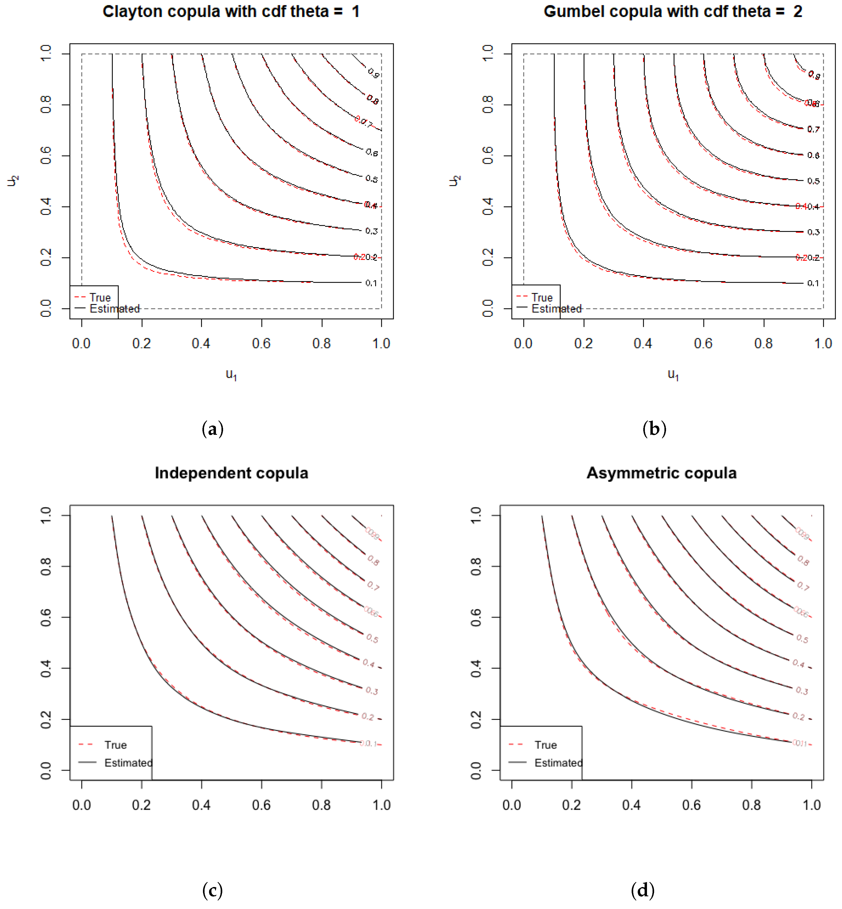
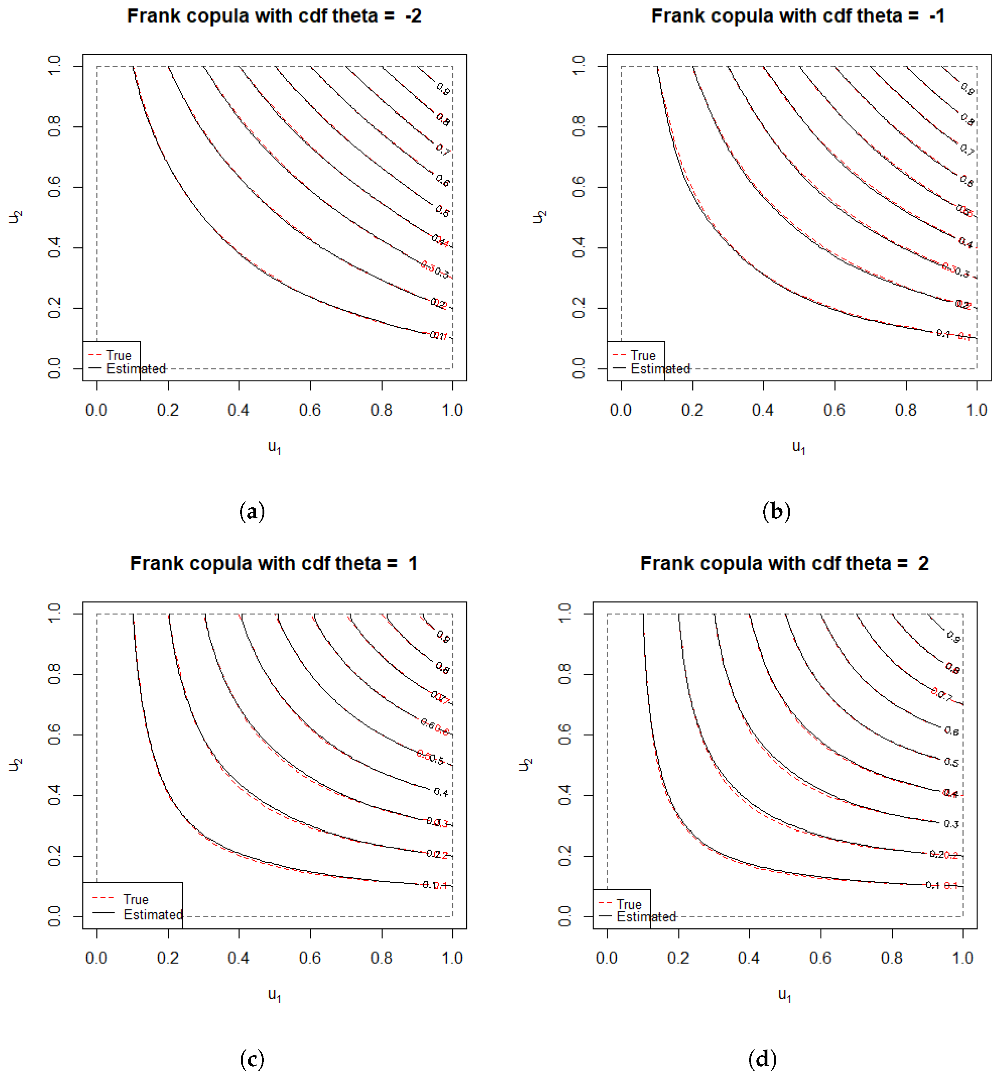
We investigate the finite-sample performance of the ECBC through a Monte Carlo simulation study. Samples from the true copula are generated using the package $\mathrm{copula}$ in $\mathrm{R}$ (Hofert et al. [34]). In order to visualize the results using contour plots, we first restrict our illustration to bivariate copulas. Three copula families with various parameters and an asymmetric copula are considered. The first four examples are the bivariate Frank copulas:

$$C_F(u,v)=-\frac{1}{\theta }ln\left(1+\frac{\left(\exp \right(-\theta u)-1)\left(\exp \right(-\theta v)-1)}{\exp (-\theta )-1)}\right),$$

with parameter $\theta$ equal to $-2,-1,1$, and 2, which reflects a wide range of dependence from negative to positive. The next two examples are the Clayton copula with parameter 1:

$$C_C(u,v)={(max\{u^{-1}+v^{-1}-1,0\})}^{-1},$$

and the Gumbel copula with parameter 2:

$$C_G(u,v)=\exp (-{({(-ln\left(u\right))}^2+{(-ln\left(v\right))}^2)}^{1/2}).$$

The value of Kendall’s tau is 0.33 for Clayton copula with parameter 1 and 0.5 for Gumbel copula with parameter 2. Both cases have a moderate positive dependence.

The next example is the independence copula $C(u,v)=uv$. Finally, we consider an asymmetric copula

$$C_a(u,v)=uv-0.12(1-v^2)\sin \left(8.3v\right)u(1-u).$$

In the simulation study, $n=100$ samples are drawn from the true copula for each replicate (of size $n=100$) and there are $N=100$ replicates. Degrees of the ECBC are estimated by posterior modes by obtaining 5000 MCMC samples following 2000 burn-in samples of two chains for each of the N replicated datasets generated from a chosen true copula model. It is to be noted that it takes about 2, 11, and 60 min to run 7000 iterations for two chains by using MacOS with 16 GB of RAM for $d=2$, $d=10$, and $d=50$, respectively, when data are drawn from multivariate Frank copula. Convergence of MCMC runs was monitored based on preliminary runs using standard diagnostics available in R packages rjags and coda. We show the results for eight copulas in Figure 1 and Figure 2. The contour plot of the true underlying copula and the empirical MC average of N copula estimates are given for comparison, and $({\overline{m}}_1,{\overline{m}}_2)$ represents the MC mean of the posterior modes of degree parameters.

We can see from the contour plots that the average of the estimated copula is extremely close to the underlying true copulas across all different dependence structures irrespective of the assumed parametric models. This illustrates that the proposed ECBC has a robust performance in estimating various true copulas.

3.2. Accuracy of Multivariate Dependence Measures (d = 3)

To assess the finite sample performance of the estimate of multivariate Spearman’s rho ${\widehat{\rho }}_d$, we conduct Monte Carlo simulations for $d=3$ copulas. We consider the independence copula and Clayton copulas with parameter value $\{0.5,1,2\}$, respectively. For each copula model, $N=100$ Monte Carlo replicates are generated with size $n=100$. For each replicate, we compute the proposed estimator ${\widehat{\rho }}_d$ in (9) and the estimator based on empirical copula ${\tilde{\rho }}_d$

$$\begin{array}{cc}\hfill {\tilde{\rho }}_d& =\frac{d+1}{2^d-(d+1)}\left(2^d{\int }_{I^d}{C}_n\left(\mathbf{u}\right)d\mathbf{u}-1\right)\hfill \\ \hfill & =\frac{d+1}{2^d-(d+1)}\left(\frac{2^d}{n}\sum _{i=1}^n\prod _{j=1}^d(1-U_{ij})-1\right).\hfill \end{array}$$

(11)

Finally, for each estimator we compute the mean, bias, variance, and mean square error (MSE) over all replicates.

Table 1. Comparison of two estimates of multivariate Spearman’s rho based on $N=100$ replications of size $n=100$ generated from the independence copula and Clayton copulas with different parameter values when dimension $d=3$.

Copula	${\mathit{\rho }}_{\mathit{d}}$	Estimator	Mean	Bias	Variance	MSE
Independence	0	${\widehat{\rho }}_d$	0.007	0.007	0.008	0.009
		${\tilde{\rho }}_d$	− 0.015	− 0.015	0.014	0.015
Clayton	0.308	${\widehat{\rho }}_d$	0.294	− 0.014	0.007	0.008
$\theta =0.5$		${\tilde{\rho }}_d$	0.287	− 0.021	0.028	0.029
Clayton	0.504	${\widehat{\rho }}_d$	0.477	−0.027	0.007	0.008
$\theta =1$		${\tilde{\rho }}_d$	0.519	0.015	0.039	0.040
Clayton	0.717	${\widehat{\rho }}_d$	0.680	−0.037	0.004	0.006
$\theta =2$		${\tilde{\rho }}_d$	0.732	0.015	0.050	0.051

shows the results of the estimation of multivariate Spearman’s rho for four different copulas. An approximated value of the true multivariate Spearman’s rho ${\rho }_d$ can be obtained by numerical integration since there is no analytical expression as a function of the parameter (see Pérez and Prieto-Alaiz [33]), which is also given in Table 1. The corresponding boxplots for the two estimates based on $N=100$ replicates along with a horizontal line for true multivariate Spearman’s rho ${\rho }_d$ are shown in Figure 3.

From the results, we can see our estimator ${\widehat{\rho }}_d$ outperforms ${\tilde{\rho }}_d$ with respect to variance and MSE. In terms of bias, ${\widehat{\rho }}_d$ tends to underestimate and have a larger bias as strength of dependence increases, but there is not a clear superiority of one estimator over the other. As shown in Figure 3c,d, where there is a moderate or strong dependence in trivariate cases, ${\tilde{\rho }}_d$ can take values out of parameter space $[-2/3,1]$ ($3\%$ and $12\%$ of ${\tilde{\rho }}_d$ are taking values greater than 1 in (c) and (d), respectively), which can be problematic in measuring dependence.

3.3. Estimation of Tuning Parameters of ECBC

We now illustrate one of the primary advantages of our proposed empirical Bayes estimate of the ECBC that allows for data-dependent automatic selection of dimension-varying degree parameters $m_j$s. We further explore the special case of choosing equal degrees $m_1=\dots =m_d=m$ by using the following prior distribution:

$$\begin{array}{c}\hfill m\mid \alpha \sim Poisson\left(n^{\alpha }\right)+1,\end{array}$$

(12)

$$\begin{array}{c}\hfill \mathrm{and}\alpha \sim Unif\left(\frac{1}{3},\frac{2}{3}\right)\end{array}$$

(13)

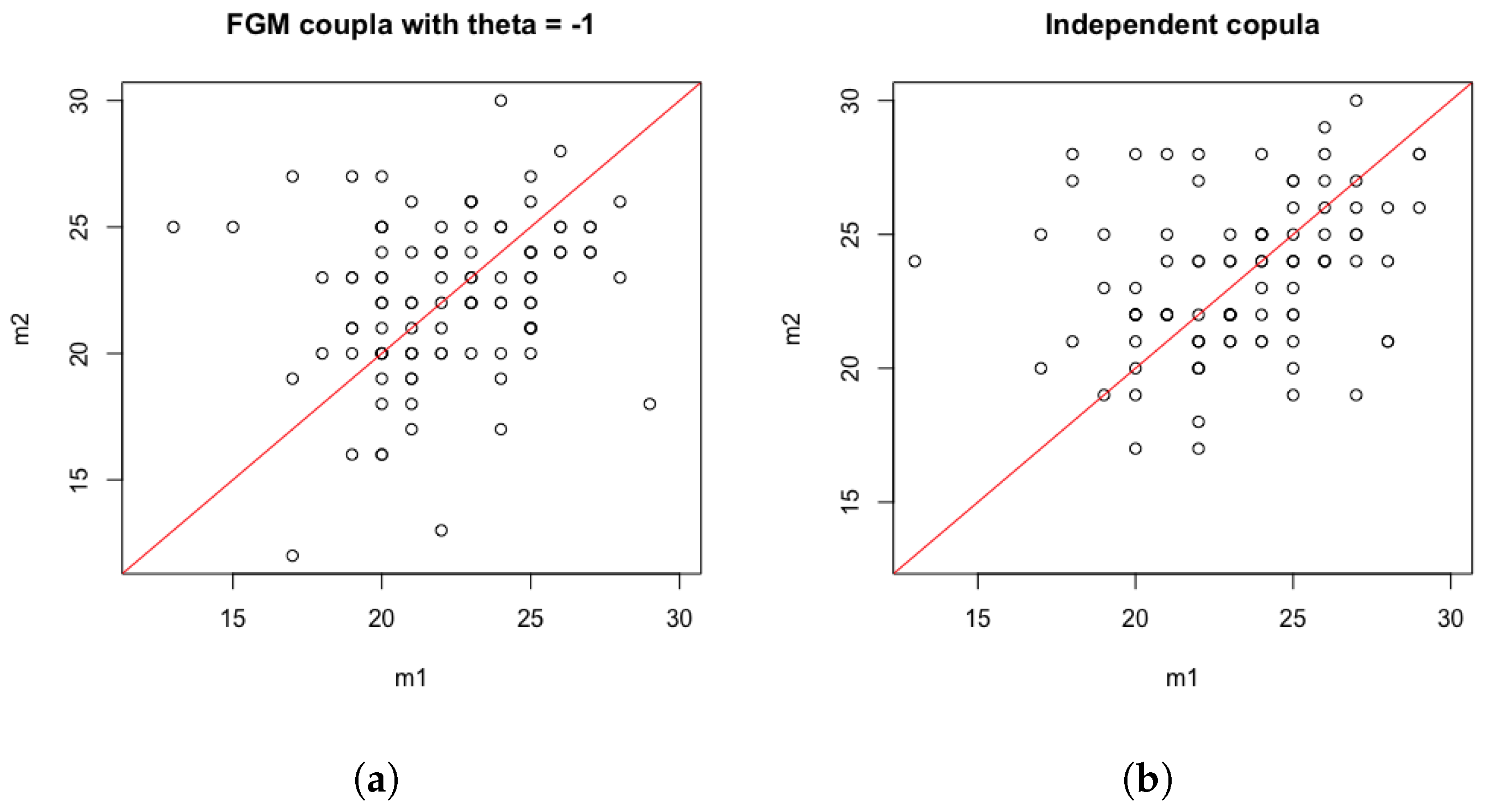
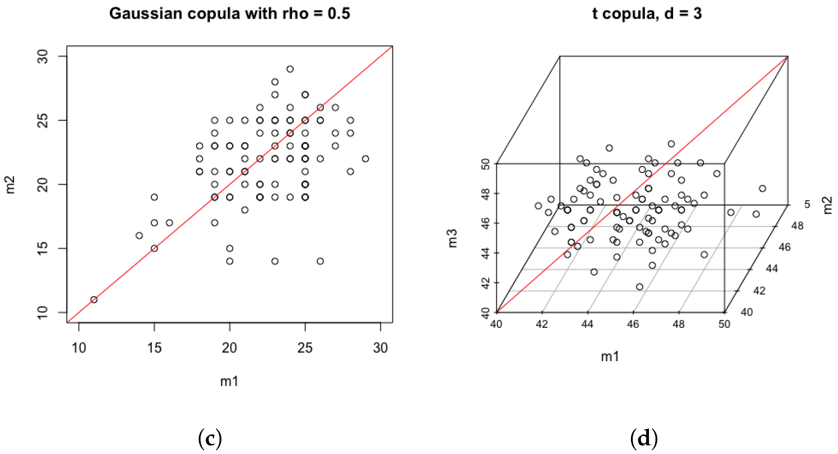
For our empirical illustration, we consider three true bivariate copulas and one trivariate copula to explore the comparative performance of choosing dimension-varying degrees compared to setting them equal across all dimensions. The first example is the Farlie–Gumbel–Morgenstern (FGM) copula $C_a(u,v)=uv(1-a(1-u)(1-v))$ with parameter $a=-1$. The next two choices are the independence copula (e.g., FGM with $a=0$) and the Gaussian copula with positive dependence (correlation $\rho =0.5$). The last one is the trivariate t-copula with four degrees of freedom and pairwise dependence ${\rho }_{12}=-0.2,{\rho }_{13}=0.5$, and ${\rho }_{23}=0.4$. Again, samples of size $n=100$ are obtained for each four cases and repeated $N=100$ times for MC evaluation. For each sample, we chose the degrees of the ECBC by computing the posterior modes using our proposed empirical Bayesian method.

Figure 4 presents the scatterplot of estimated values of $(m_1,m_2)$ or $(m_1,m_2,m_3)$ for each chosen true copula model. From the plots, we can observe that for bivariate copulas, posterior estimates of $m_1$ and $m_2$ are significantly different in most cases without any prior restrictions of equality. In fact, posterior probability of choosing equal $m_1=m_2$ is only about $0.08,0.08$, and $0.13$ for FGM copula, for independence copula, and for Gaussian copula, respectively, indicating against forcing $m_1=m_2$, as is popularly performed in the literature. For the trivariate t-copula case, the posterior probability of $m_1=m_2=m_3$ is 0, decisively suggesting that equality assumption is suboptimal in general and particularly as the dimension increases. We conducted further studies with dimensions (not shown here for limitation of space) and the conclusions remain very similar.

In order to further compare the performances of copula estimators with flexible degrees vs. equal degrees, we fit our Bayesian models with two different settings of priors: (i) (flexible) the original priors given in (6) and (7), where degrees are allowed to vary in different dimensions; (ii) (equal) modified priors given in (12) and (13), where degrees are set to be equal; using the same dataset generated from the three bivariate copulas. Following Segers et al. [22], we consider three global performance measures: the integrated squared bias, the integrated variance, and the integrated mean squared error. Given a copula estimator ${\widehat{C}}_n$, the performance measures are defined as

$$\begin{array}{ccc}\hfill \mathrm{integrated}\mathrm{squared}\mathrm{bias}:ISB& =& {\int }_{{[0,1]}^d}{\left[E[{\widehat{C}}_n\left(\mathbf{u}\right)-C\left(\mathbf{u}\right)]\right]}^{2}d\mathbf{u},\hfill \\ \hfill \mathrm{integrated}\mathrm{variance}:IV& =& {\int }_{{[0,1]}^d}E\left[{[{\widehat{C}}_n\left(\mathbf{u}\right)-E\left({\widehat{C}}_n\left(\mathbf{u}\right)\right)]}^2\right]d\mathbf{u},\hfill \\ \hfill \mathrm{integrated}\mathrm{mean}\mathrm{squared}\mathrm{error}:IMSE& =& {\int }_{{[0,1]}^d}E\left[{[{\widehat{C}}_n\left(\mathbf{u}\right)-C\left(\mathbf{u}\right)]}^2\right]d\mathbf{u}.\hfill \end{array}$$

We compute the performance measures by applying the computation method described in Segers et al. [22], which relies on Monte Carlo simulation to obtain a Monte Carlo estimate of each performance measure.

Table 2. Comparison of copula estimators with flexible degrees vs. equal degrees using three performance measures computed by Monte Carlo simulation based on $N=100$ replications when sample size $n=100.$

Copula	Choice of Degrees	ISB ($\times {10}^{-4}$)	IV ($\times {10}^{-4}$)	IMSE ($\times {10}^{-4}$)
FGM	Flexible	$0.10$	$1.28$	$1.38$
$\theta =-1$	Equal	$0.09$	$1.37$	$1.46$
Independence	Flexible	$0.13$	$1.89$	$2.02$
	Equal	$0.20$	$2.16$	$2.36$
Gaussian	Flexible	$0.36$	$0.71$	$1.07$
$\rho =0.5$	Equal	$0.30$	$0.83$	$1.13$
t	Flexible	$0.11$	$2.67$	$2.78$
$d=3$	Equal	$0.19$	$2.79$	$2.98$

presents the results for the four cases, where the first three are bivariate ($d=2$) and the last one is trivariate ($d=3$). The standard errors of the Monte Carlo estimates are not reported in the table as they are negligibly small. We can see that the copula estimators with flexible degrees perform better than those with equal degrees in terms of IV and IMSE in all cases. As the difference in IMSE is dominated by the IV term, the choice of flexible degrees leads to smaller uncertainty, and hence smaller IMSE, while the biases remain relatively unaffected. It is also interesting to observe that estimated degrees are far smaller than sample sizes, indicating that the empirical beta copula may not have optimal performance, which we explore next.

3.4. Comparison with the Empirical Bernstein Copulas

In this section, we compare the finite-sample performance of the ECBC with other nonparametric copula estimators only, as it has been already demonstrated that parametric-model-based methods lead to biased estimates under model misspecification. First, we consider the empirical beta copula introduced by Segers et al. [22], which is a special case of the empirical Bernstein copula where the degrees of the polynomials are set equal to the sample size. The empirical beta copula is a genuine copula and has been shown to outperform the classical empirical copula and the empirical checkerboard copula in terms of bias and variance. For bivariate cases, we also include the empirical Bernstein copula with degrees, as suggested in Janssen et al. [19], into the comparison. By setting degrees $m_1=m_2=m$ and minimizing the asymptotic pointwise mean squared error with respect to m, Janssen et al. [19] suggested the choice of m in the bivariate case as

$$m_0(u_1,u_2)={\left(\frac{4b^2(u_1,u_2)}{V(u_1,u_2)}\right)}^{2/3}{n}^{2/3}$$

(14)

where

$$\begin{array}{ccc}\hfill b^2(u_1,u_2)& =& \frac{1}{2}\sum _{j=1}^2{u}_j(1-u_j)C_{u_j{u}_j}(u_1,u_2)\hfill \\ \hfill \mathrm{and}V(u_1,u_2)& =& \sum _{j=1}^2{C}_{u_j}(u_1,u_2)(1-C_{u_j}(u_1,u_2)){\left(\frac{u_j(1-u_j)}{\pi }\right)}^{1/2}\hfill \end{array}$$

and $C_{u_j}$ and $C_{u_j{u}_j}$ are the first-order and second-order partial derivatives of C, respectively, with respect to $u_j,j=1,2$. Note that even we use the integer part $\lfloor m_0(u_1,u_2)\rfloor$ in practice; it is not necessarily a divisor of n, meaning that the empirical Bernstein copula with $m=\lfloor m_0(u_1,u_2)\rfloor$ is not guaranteed to be a genuine copula.

We consider the same copula models as in Section 3.3. The choice of degrees $m_0(u_1,u_2)$, suggested by Janssen et al. [19], is not defined for the independence copula as $C_{u_j{u}_j}=0$ and it is restricted to bivariate cases, so we only take the empirical Bernstein copula into consideration for the bivariate FGM and Gaussian copulas. All results in

Table 3. Comparison of the ECBC with flexible degrees (referred to as flexible ECBC), the empirical beta copula (referred to as Beta), and the empirical Bernstein copula with $m=m_0(u_1,u_2)$ (referred to as Bernstein) using three performance measures computed by Monte Carlo simulation based on $N=100$ replications for sample size $n=25,50,100$.

		ISB ($\times {10}^{-4}$)			IV ($\times {10}^{-4}$)			IMSE ($\times {10}^{-4}$)
Copula	Estimator	n =			n =			n =
		25	50	100	25	50	100	25	50	100
FGM	flexible ECBC	0.29	0.07	0.10	3.46	2.72	1.28	3.75	2.79	1.38
$\theta =-1$	Beta	0.30	0.09	0.02	5.24	3.27	2.17	5.54	3.36	2.19
	Bernstein	0.83	0.51	0.07	1.52	1.33	1.08	2.35	1.84	1.15
Independence	flexible ECBC	0.68	0.31	0.13	2.37	2.33	1.89	3.05	2.64	2.02
	Beta	0.02	0.03	0.01	5.11	4.02	2.25	5.13	4.05	2.26
	Bernstein	NA	NA	NA	NA	NA	NA	NA	NA	NA
Gaussian	flexible ECBC	1.72	0.79	0.36	2.51	1.67	0.71	4.23	2.46	1.07
$\rho =0.5$	Beta	0.26	0.16	0.20	4.78	3.03	1.81	5.04	3.19	2.01
	Bernstein	6.82	3.09	1.27	2.28	1.42	1.06	9.10	4.51	2.33
t	flexible ECBC	0.41	0.30	0.11	6.76	4.26	2.67	7.17	4.56	2.78
$d=3$	Beta	0.27	0.15	0.04	7.55	5.05	3.07	7.82	5.20	3.11
	Bernstein	NA	NA	NA	NA	NA	NA	NA	NA	NA

are based on $N=100$ MC replications each of sample sizes $n=25,50,100$. We compare the performance of the ECBC with flexible degrees (referred to as flexible ECBC), the empirical beta copula (referred to as Beta), and the empirical Bernstein copula with $m=m_0(u_1,u_2)$ (referred to as Bernstein) using the same performance measures as in Section 3.3.

Table 3 indicates that the ECBC with flexible degrees outperforms the empirical beta copula in terms of variance and mean square error in all cases. Compared to the empirical Bernstein copula with $m=m_0(u_1,u_2)$, the ECBC with flexible degrees has a smaller bias but the ordering with respect to mean square error is not clear between these two copula estimators. For small samples, the empirical beta copula seems to have the largest variance while the bias of the empirical Bernstein copula with $m=m_0(u_1,u_2)$ is shown to be the largest, even though it uses optimal “true” degree given in (14).

4. Application to Portfolio Risk Management

Copulas have been widely used in portfolio optimization and risk measurement as they are powerful tools to model the dependence among different assets in a portfolio. The proposed ECBC is capable of estimating multivariate copula and it is straightforward to sample from the estimated copula, so it can be applied to find optimal weights and estimate risk measures for a portfolio with a variety of assets.

We now illustrate the use of ECBC for portfolio risk allocation using real data consisting of a d asset values. Value at risk (VaR) and conditional value at risk (CVaR) (also called expected shortfall (ES)) are common measures of risk in the field of risk management (see, e.g., Jorion [35] and Uryasev [36]). Assume that X is the return of a portfolio or asset (daily log-return of a portfolio of stocks or individual stocks, with positive indicating profit and negative values representing loss) with distribution function $F_X(·)=Pr[X\le x]$. The VaR of X at the level of $\alpha \in (0,1)$ is defined as

$$\begin{array}{c}\hfill Va{R}_{\alpha }\left(X\right)=-inf\{x\in \mathbb{R}:F_X\left(x\right)>\alpha \},\end{array}$$

while the CVaR (ES) of X is defined as

$$\begin{array}{c}\hfill CVa{R}_{\alpha }\left(X\right)=E(-X|X\le -Va{R}_{\alpha }\left(X\right)).\end{array}$$

Notice that, if we consider the corresponding loss of the same portfolio represented by $Y=-X$, then we have $Va{R}_{\alpha }\left(X\right)=Va{R}_{\alpha }\left(Y\right)=F_Y^{-1}(1-\alpha )$ and $CVa{R}_{\alpha }\left(X\right)=CVa{R}_{\alpha }\left(Y\right)=E\left(Y\right|Y\ge Va{R}_{\alpha }\left(Y\right))$.

Mean-CVaR portfolio optimization is a popular portfolio optimization technique introduced by Rockafellar et al. [37]. The advantage of mean-CVaR portfolio optimization is that it calculates VaR and minimizes CVaR simultaneously, where the optimization can be formulated as a linear programming problem.

Let $\mathbf{x}\in {\mathbb{R}}^d$ denote a realized return value of d assets in a portfolio, and $\mathbf{v}\in {\mathcal{S}}_d=\{\mathbf{v}\in {\mathbb{R}}^d:v_j\ge 0,\forall j,{\sum }_{j=1}^d{v}_j=1\}$ denote the portfolio weights to be determined within the d-dimensional simplex ${\mathcal{S}}_d$. The key to the approach in Rockafellar et al. [37] is the auxiliary function for CVaR taking the form of

$$\begin{array}{c}\hfill H_{\alpha }(\mathbf{v},\gamma )=\gamma +\frac{1}{\alpha }{\int }_{l(\mathbf{v},\mathbf{x})\ge \gamma }(l(\mathbf{v},\mathbf{x})-\gamma )dF\left(\mathbf{x}\right),\end{array}$$

(15)

where $l(\mathbf{v},\mathbf{x})=-{\mathbf{v}}^T\mathbf{x}$ is a linear loss function and $F\left(\mathbf{x}\right)$ is the joint distribution function of daily (random) return vector $\mathbf{X}$, which we will estimate using our proposed ECBC-based empirical Bayes method. It was shown in Theorem 1 of Rockafellar et al. [37] that for any weights $\mathbf{v}$, $H_{\alpha }(\mathbf{v},\gamma )$ is convex as a function of $\gamma$ and is equal to $CVa{R}_{\alpha }\left(\mathbf{v}\right)$ at the minimum point. Moreover, $Va{R}_{\alpha }\left(\mathbf{v}\right)$ would be the left endpoint of $\underset{\gamma }{argmin}{H}_{\alpha }(\mathbf{v},\gamma )$. Moreover, minimizing $CVa{R}_{\alpha }\left(\mathbf{v}\right)$ with respect to $\mathbf{v}$ is equivalent to minimizing $H_{\alpha }(\mathbf{v},\gamma )$ with respect to $(\mathbf{v},\gamma )$ (e.g., see Theorem 2 of Rockafellar et al. [37] for details). To numerically approximate the integral in (15), it is often good enough to generate M samples from $F(·)$ or its estimate, which can be performed by using the proposed empirical Bayes method based on the ECBC. However, a relatively less-answered question in finance is how large we should choose M for accurate estimation, as the integral in (15) depends on sampling the tail part of $F(·)$ or its estimate. The empirical estimate of $H_{\alpha }(\mathbf{v},\gamma )$ based on generating ${\mathbf{x}}_k\stackrel{iid}{\sim }F$ or $\widehat{F}$ can be written as

$$\begin{array}{c}\hfill F_{\alpha }(\mathbf{v},\gamma )=\gamma +\frac{1}{\alpha M}\sum _{k=1}^M{(-{\mathbf{v}}^T{\mathbf{x}}_k-\gamma )}_{+}\end{array}$$

(16)

where ${(·)}_{+}=max(·,0)$.

Proposition 1.

In order to achieve an accuracy of $ϵ>0$ for the MC approximation, it is sufficient to generate M MC samples such that

$$\begin{array}{c}\hfill \sqrt{\frac{2lnlnM}{M}{\lambda }_{max}}\le ϵ,i.e.,\frac{M}{lnlnM}\ge \frac{2{\lambda }_{max}}{{ϵ}^2}\end{array}$$

(17)

where $\Sigma =Va{r}_F\left(\mathbf{X}\right)$ and ${\lambda }_{max}$ is the largest eigenvalue of Σ.

Proof. 

By the law of the iterated logarithm (see, e.g., Balsubramani [38]), the deviation of MC approximation from the mean is almost surely bounded by

$$\begin{array}{c}\hfill \sqrt{\frac{2lnlnM}{M}}\sqrt{Var\left({(-{\mathbf{v}}^T{\mathbf{x}}_k-\gamma )}_{+}\right)}\end{array}$$

Let $\Sigma =Va{r}_F\left(\mathbf{X}\right)$ and ${\lambda }_{max}$ be the largest eigenvalue of $\Sigma$, then we have

$$\begin{array}{c}\hfill Var\left({(-{\mathbf{v}}^T\mathbf{X}-\gamma )}_{+}\right)\le Var\left({\mathbf{v}}^T\mathbf{X}\right)={\mathbf{v}}^T\Sigma \mathbf{v}\le {\lambda }_{max}{\mathbf{v}}^T\mathbf{v}\le {\lambda }_{max},\end{array}$$

for any $\mathbf{v}\in {\mathcal{S}}_d$, because ${\mathbf{v}}^T\mathbf{v}\le {\mathbf{v}}^T\mathbf{1}=1$. Thus, for an accuracy of $ϵ>0$ for the MC approximation, it is sufficient to generate M MC samples such that

$$\begin{array}{c}\hfill \sqrt{\frac{2lnlnM}{M}{\lambda }_{max}}\le ϵ,i.e.,\frac{M}{lnlnM}\ge \frac{2{\lambda }_{max}}{{ϵ}^2}\end{array}$$

   □

Notice that $\Sigma$, and hence ${\lambda }_{max}$, can be easily estimated from the observed return values without any modeling assumption as long as $n>d$; however, sparse methods are necessary for large-sized portfolios when $n\le d$. Next, it is shown that minimizing (16) is equivalent to minimizing

$$\begin{array}{c}\hfill F_{\alpha }(\mathbf{v},\gamma )=\gamma +\frac{1}{\alpha M}\sum _{k=1}^M{z}_{k}s.t.z_k\ge 0,z_k+{\mathbf{v}}^T{\mathbf{x}}_k+\gamma \ge 0\end{array}$$

(18)

Thus, along with the linear constraints on the weights $\mathbf{v}$, it can be formulated as a linear programming problem and can be solved using standard convex optimization methods. Conveniently, $\mathrm{R}$ function $\mathrm{BDportfolio}\_\mathrm{optim}$ within the package $\mathrm{PortfolioOptim}$ can be used for this purpose. Following the algorithm in Semenov and Smagulov [39], simulated return values can be obtained using estimated ECBC for portfolio optimization. The complete algorithm is summarized below:

Step 1. Transform assets’ historical data $X_{tj}$ to pseudo-observations $U_{tj}$ and estimate copula using our proposed method.

$$U_{tj}=F_{Tj}^{\ast }\left(X_{tj}\right),t=1,\dots ,T,j\in \{1,\cdots ,d\},$$

$$F_{Tj}^{\ast }\left(x_j\right)=\frac{1}{T+1}\sum _{t=1}^{T}I(X_{tj}\le x_j),j\in \{1,\cdots ,d\}.$$

Step 2. Generate a sample of pseudo-observations $(U_{k1}^{\ast },\dots ,U_{kd}^{\ast }),k=1,\dots ,M$ from the estimated ECBC using empirical Bayes method and transform simulated pseudo-observations to univariate quantiles.

$$X_{kj}^{\ast }=F_{Tj}^{\ast -1}\left(U_{kj}^{\ast }\right),k=1,\dots ,M,j\in \{1,\cdots ,d\}.$$

Step 3. Calculate optimal weights $v_j,j\in \{1,\cdots ,d\}$ using simulated data $(X_{k1}^{\ast },\dots ,X_{kd}^{\ast })$, $k=1,\dots ,M$, and the corresponding VaR and CVaR, which are byproducts of the portfolio optimization, by solving the linear programming problem given in (18).

Our copula estimator is useful to find optimal weights and estimate risk measures as sampling from the estimated copula is straightforward. Considering the Bernstein copula density given in (4) and (5), we can obtain samples $(U_1,\dots U_d)\sim C_m$ as follows:

$$\begin{array}{cc}\hfill (k_1,\dots ,k_d)& \sim {\tilde{w}}_{k_1,\dots ,k_d},k_j\in \{0,\dots ,m_j-1\},j\in \{1,\cdots ,d\}\hfill \\ \hfill U_j& \sim \mathrm{Beta}(k_j+1,m_j-k_j),j\in \{1,\cdots ,d\}\hfill \end{array}$$

As an example with moderately large dimension, we investigate the time series of daily closing stock prices of the 10 top Nasdaq companies: AMZN, FB, GOOGL, AAPL, MSFT, INTC, CSCO, NFLX, CMCSA, and ADBE for the time period from 1 January 2018 to 31 December 2019. This dataset consists of 502 observations and can be obtained using $\mathrm{R}$ package $\mathrm{quantmod}$.

Suppose we want to find an optimal portfolio of stocks above that minimizes the expected shortfall of the portfolio. First, we convert the price series $P_{tj}$ to log-returns $X_{tj}$

$$\begin{array}{c}\hfill X_{tj}=ln\frac{P_{tj}}{P_{(t-1)j}},t=1,\dots ,T,j\in \{1,\cdots ,d\},\end{array}$$

resulting in $T=501$ log-return values for $d=10$ assets. Then we follow Steps 1–3 as above to obtain the optimal portfolio weights and the corresponding VaR and CVaR. Similar to Semenov and Smagulov [39], we set the minimum weight to be limited by $v_j\ge 0.01,j\in \{1,\cdots ,d\}$ to avoid corner portfolio cases.

In Step 1, the posterior mode estimators of the degrees of the proposed ECBC are $(209,206,208,206,208,209,211,$$210,209,$$208)$. The largest eigenvalue of the covariance matrix is ${\lambda }_{max}\approx 2\times {10}^{-3}$, so we are able to find the value of M that is sufficient for a given accuracy $ϵ$ from the relationship in (17).

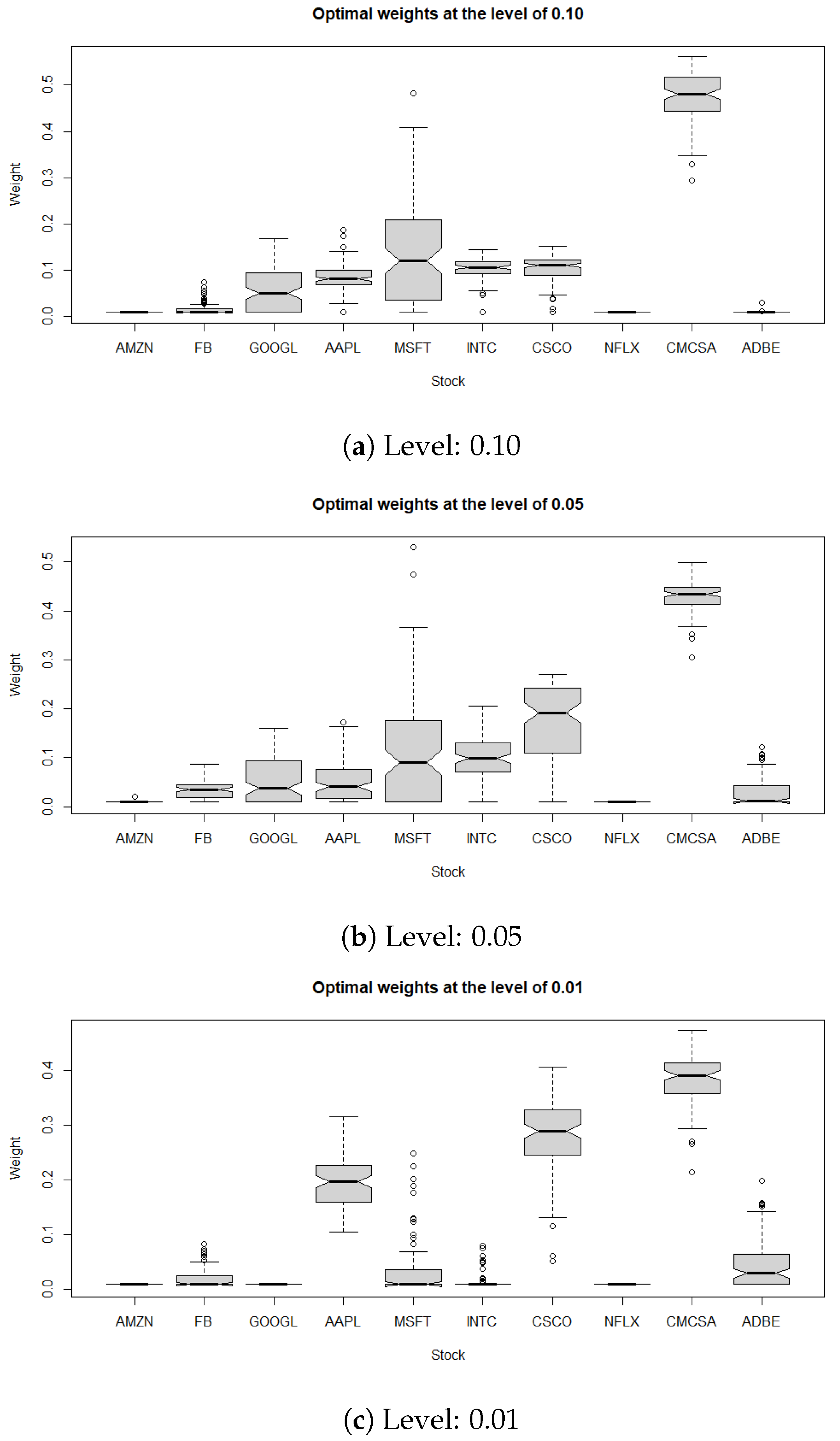
We set $M=\mathrm{10,000}$ (adequate for an accuracy $ϵ\approx 9\times {10}^{-4}$) and repeat Steps 2–3 $N=100$ times to quantify estimation uncertainty. For each replicate we conduct portfolio optimization at the level of $\alpha \in \{0.10,0.05,0.01\}$ as popularly used. As a result, we are able to obtain the distribution of optimal weights (Figure 5) and risk measures (Figure 6) using simulated data from the estimated copula.

From the boxplots of optimal weights in Figure 5 we can see that CMCSA has a much higher weight than the other stocks in the mean-CVaR optimal portfolio across different levels. Also, by applying mean-CVaR portfolio optimization to the historical log-return data $X_{tj}$, we can obtain estimates of optimal weights and risk measures as well. In Figure 6, the dashed lines indicate empirical estimates of risk measures using historical data.

We can see from the plots in Figure 6 that the estimated risk measures from two different methods seem to be fairly close. However, we are able to quantify the uncertainty for all the estimates by repeatedly sampling from the estimated copula. Semenov and Smagulov [39] conducted a similar stability study to report the means and SDs of VaR and CVaR, but they used predetermined weights based on historical data and did not report the distribution of optimal weights obtained from simulated data. Our copula estimator shows good performance for relatively small samples, and operationally, we can generate as many samples as we want from the estimated copula; thus, the copula-based method would be more reliable when there are not sufficient historical data. In addition, compared to the empirical estimates, it is possible to estimate VaR and CVaR for much smaller values of levels using the copula-based method.

5. Concluding Remarks

In this paper, we proposed the empirical checkerboard Bernstein copula, which is a nonparametric multivariate copula estimator. It can be considered as an advancement of the empirical Bernstein copula since it is a valid copula with any polynomial degrees for any sample size. For automatic data-dependent dimension-varying degree selections, we further developed an empirical Bayesian method that was shown to be practically useful. While the proposed copula estimator was shown to be large-sample consistent, it also had a good finite-sample performance. Moreover, it had a beneficial effect on measuring the strength of dependence for large dimensions because the estimates derived from the proposed copula were always within the proper range.

As sampling from the estimated copula is quite straightforward, it is applicable to portfolio optimization and risk measurement where estimation is often performed with simulations generated from copulas. We investigated the number of simulations that were good enough to achieve any given accuracy, which was apparently out of reach in the literature. Furthermore, we were able to provide uncertainty quantification for all the estimates in portfolio risk management.

Under the hierarchical structure of the proposed empirical Bayes model, MCMC methods have been shown to work reasonably fast for relatively large dimensions ($d\le 50$) with a moderate sample size ($n=100$). To speed up the MCMC methods for very large sample sizes, it would be of interest to explore some scalable MCMC methods such as divide-and-conquer approaches and subsampling approaches (see, e.g.,  Quiroz et al. [40], Robert et al. [41], etc.). The code (written using R software) to implement the procedure is available upon request from the first author and could be made available on a GitHub page following the publication of this paper.

References

1. Jaworski, P.; Durante, F.; Hardle, W.K.; Rychlik, T. Copula Theory and Its Applications; Springer: Berlin/Heidelberg, Germany, 2010; Volume 198. [Google Scholar]
2. Joe, H. Dependence Modeling with Copulas; Chapman and Hall/CRC: New York, NY, USA, 2014. [Google Scholar]
3. Nelsen, R.B. An Introduction to Copulas; Springer: Berlin/Heidelberg, Germany, 2007. [Google Scholar]
4. Sklar, M. Fonctions de repartition an dimensions et leurs marges. Publ. Inst. Statist. Univ. Paris 1959, 8, 229–231. [Google Scholar]
5. Joe, H. Asymptotic efficiency of the two-stage estimation method for copula-based models. J. Multivar. Anal. 2005, 94, 401–419. [Google Scholar] [CrossRef]
6. McNeil, A.J.; Nešlehová, J. Multivariate Archimedean copulas, d-monotone functions and l1-norm symmetric distributions. Ann. Stat. 2009, 37, 3059–3097. [Google Scholar] [CrossRef] [PubMed]
7. Smith, M.S. Bayesian approaches to copula modelling. arXiv 2011, arXiv:1112.4204. [Google Scholar] [CrossRef]
8. Žežula, I. On multivariate Gaussian copulas. J. Stat. Plan. Inference 2009, 139, 3942–3946. [Google Scholar] [CrossRef]
9. Deheuvels, P. La fonction de dépendance empirique et ses propriétés. Un test non paramétrique d’indépendance. Bull. L’Académie R. Belg. 1979, 65, 274–292. [Google Scholar] [CrossRef]
10. Fermanian, J.D.; Radulovic, D.; Wegkamp, M. Weak convergence of empirical copula processes. Bernoulli 2004, 10, 847–860. [Google Scholar] [CrossRef]
11. Genest, C.; Nešlehová, J.G.; Rémillard, B. Asymptotic behavior of the empirical multilinear copula process under broad conditions. J. Multivar. Anal. 2017, 159, 82–110. [Google Scholar] [CrossRef]
12. Chen, S.X.; Huang, T.M. Nonparametric estimation of copula functions for dependence modelling. Can. J. Stat. 2007, 35, 265–282. [Google Scholar] [CrossRef]
13. Gijbels, I.; Mielniczuk, J. Estimating the density of a copula function. Commun. Stat.-Theory Methods 1990, 19, 445–464. [Google Scholar] [CrossRef]
14. Omelka, M.; Gijbels, I.; Veraverbeke, N. Improved kernel estimation of copulas: Weak convergence and goodness-of-fit testing. Ann. Stat. 2009, 37, 3023–3058. [Google Scholar] [CrossRef]
15. Rémillard, B.; Scaillet, O. Testing for equality between two copulas. J. Multivar. Anal. 2009, 100, 377–386. [Google Scholar] [CrossRef]
16. Scaillet, O.; Fermanian, J.D. Nonparametric estimation of copulas for time series. FAME Res. Pap. 2002. [Google Scholar] [CrossRef]
17. Wu, J.; Wang, X.; Walker, S.G. Bayesian nonparametric inference for a multivariate copula function. Methodol. Comput. Appl. Probab. 2014, 16, 747–763. [Google Scholar] [CrossRef]
18. Sancetta, A.; Satchell, S. The Bernstein copula and its applications to modeling and approximations of multivariate distributions. Econom. Theory 2004, 20, 535–562. [Google Scholar] [CrossRef]
19. Janssen, P.; Swanepoel, J.; Veraverbeke, N. Large sample behavior of the Bernstein copula estimator. J. Stat. Plan. Inference 2012, 142, 1189–1197. [Google Scholar] [CrossRef]
20. Belalia, M.; Bouezmarni, T.; Lemyre, F.; Taamouti, A. Testing independence based on Bernstein empirical copula and copula density. J. Nonparametr. Stat. 2017, 29, 346–380. [Google Scholar] [CrossRef]
21. Diers, D.; Eling, M.; Marek, S.D. Dependence modeling in non-life insurance using the Bernstein copula. Insur. Math. Econ. 2012, 50, 430–436. [Google Scholar] [CrossRef]
22. Segers, J.; Sibuya, M.; Tsukahara, H. The empirical beta copula. J. Multivar. Anal. 2017, 155, 35–51. [Google Scholar] [CrossRef]
23. Burda, M.; Prokhorov, A. Copula based factorization in Bayesian multivariate infinite mixture models. J. Multivar. Anal. 2014, 127, 200–213. [Google Scholar] [CrossRef]
24. Lu, L.; Ghosh, S.K. Nonparametric Estimation and Testing for Positive Quadrant Dependent Bivariate Copula. J. Bus. Econ. Stat. 2020, 40, 664–677. [Google Scholar] [CrossRef]
25. Embrechts, P.; Lindskog, F.; McNeil, A. Modelling dependence with copulas. Rapp. Tech. Département Mathématiques Inst. Fédéral Technol. Zur. 2001, 14, 1–50. [Google Scholar]
26. Carley, H.; Taylor, M. A New Proof of Sklar’s Theorem; Springer: Berlin/Heidelberg, Germany, 2002; pp. 29–34. [Google Scholar]
27. Li, X.; Mikusiński, P.; Sherwood, H.; Taylor, M. On Approximation of Copulas; Springer: Berlin/Heidelberg, Germany, 1997; pp. 107–116. [Google Scholar]
28. Gijbels, I.; Omelka, M.; Sznajder, D. Positive quadrant dependence tests for copulas. Can. J. Stat. 2010, 38, 555–581. [Google Scholar] [CrossRef]
29. Janssen, P.; Swanepoel, J.; Veraverbeke, N. A note on the asymptotic behavior of the Bernstein estimator of the copula density. J. Multivar. Anal. 2014, 124, 480–487. [Google Scholar] [CrossRef]
30. Kiriliouk, A.; Segers, J.; Tsukahara, H. On some resampling procedures with the empirical beta copula. arXiv 2019, arXiv:1905.12466. [Google Scholar]
31. Berger, J.O.; Liseo, B.; Wolpert, R.L. Integrated likelihood methods for eliminating nuisance parameters. Stat. Sci. 1999, 14, 1–28. [Google Scholar] [CrossRef]
32. Nelsen, R.B. Nonparametric measures of multivariate association. Lect. Notes Monogr. Ser. 1996, 223–232. [Google Scholar]
33. Pérez, A.; Prieto-Alaiz, M. A note on nonparametric estimation of copula-based multivariate extensions of Spearman’s rho. Stat. Probab. Lett. 2016, 112, 41–50. [Google Scholar] [CrossRef]
34. Hofert, M.; Kojadinovic, I.; Maechler, M.; Yan, J.; Maechler, M.M.; Suggests, M. Package ‘Copula’. 2014. Available online: http://ie.archive.ubuntu.com/disk1/disk1/cran.r-project.org/web/packages/copula/copula.pdf (accessed on 12 September 2023).
35. Jorion, P. Value at Risk: The New Benchmark for Managing Financial Risk; McGraw Hill: New York, NY, USA, 2007. [Google Scholar]
36. Uryasev, S. Conditional Value-at-Risk: Optimization Algorithms and Applications; Springer: Berlin/Heidelberg, Germany, 2000; pp. 49–57. [Google Scholar]
37. Rockafellar, R.T.; Uryasev, S. Optimization of conditional value-at-risk. J. Risk 2000, 2, 21–42. [Google Scholar] [CrossRef]
38. Balsubramani, A. Sharp finite-time iterated-logarithm martingale concentration. arXiv 2014, arXiv:1405.2639. [Google Scholar]
39. Semenov, M.; Smagulov, D. Portfolio risk assessment using copula models. arXiv 2017, arXiv:1707.03516. [Google Scholar]
40. Quiroz, M.; Kohn, R.; Villani, M.; Tran, M.N. Speeding up MCMC by efficient data subsampling. J. Am. Stat. Assoc. 2018, 16, 831–843. [Google Scholar]
41. Robert, C.P.; Elvira, V.; Tawn, N.; Wu, C. Accelerating MCMC algorithms. Wiley Interdiscip. Rev. Comput. Stat. 2018, 10, e1435. [Google Scholar] [CrossRef] [PubMed]
Figure 1. Estimation of Frank copulas using the ECBC with empirical Bayesian method for choosing proper degrees when sample size n = 100 . (a) ( m ¯ 1 , m ¯ 2 ) = ( 22.52 , 24.01 ) , (b) ( m ¯ 1 , m ¯ 2 ) = ( 22.46 , 23.17 ) , (c) ( m ¯ 1 , m ¯ 2 ) = ( 23.29 , 24.83 ) , (d) ( m ¯ 1 , m ¯ 2 ) = ( 22.82 , 22.17 ) .
Mathematics 11 04383 g001
Figure 2. Estimation of various copulas using the ECBC with empirical Bayesian method for choosing proper degrees when sample size n = 100 . (a) ( m ¯ 1 , m ¯ 2 ) = ( 23.94 , 21.69 ) , (b) ( m ¯ 1 , m ¯ 2 ) = ( 22.58 , 22.16 ) , (c) ( m ¯ 1 , m ¯ 2 ) = ( 22.34 , 20.87 ) , (d) ( m ¯ 1 , m ¯ 2 ) = ( 21.08 , 22.92 ) .
Mathematics 11 04383 g002
Figure 3. Boxplots of the two estimators based on N = 100 replicates and a horizontal line of true multivariate Spearman’s rho ρ d for each of four trivariate copulas.
Mathematics 11 04383 g003
Figure 4. Choice of dimension-varying degrees obtained by applying the proposed empirical Bayesian method based on N = 100 replications when sample size n = 100 .
Mathematics 11 04383 g004aMathematics 11 04383 g004b
Figure 5. Distribution of optimal weights obtained from simulated data using the estimated copula at the level of 0.10 , 0.05 , and 0.01 , for a portfolio of d = 10 stocks.
Mathematics 11 04383 g005
Figure 6. Distribution of VaR and CVaR obtained from simulated data using the estimated copula at the level of 0.10 , 0.05 , and 0.01 for a portfolio of d = 10 stocks. Dashed lines indicate empirical estimates using historical data.
Mathematics 11 04383 g006