Ultimate Dynamics of the Two-Phenotype Cancer Model: Attracting Sets and Global Cancer Eradication Conditions

Abstract

In this paper we consider the ultimate dynamics of one 4D cancer model which was created for studying the immune response to the two-phenotype tumors. Our approach is based on the localization method of compact invariant sets. The existence of a positively invariant polytope is shown and its size is calculated depending on the parameters of this cancer model. Various convergence conditions to the tumor free equilibrium point were proposed. This property has the biological meaning of global asymptotic tumor eradication (GATE). Further, the case in which local asymptotic tumor eradication (LATE) conditions entail GATE conditions was found. Our theoretical studies of ultimate dynamics are complemented by numerical simulation results.

1. Introduction

Human cancers often demonstrate significant intra-tumor heterogeneity in almost all distinguishable phenotypic features, such as cellular morphology, gene expression (including expression of cell surface markers, growth factor receptors and hormones), metabolism, motility and angiogenic, proliferative, immunogenic and metastatic potential [1,2,3,4,5,6]. Taking into account such features leads to a significant complication of mathematical models of the interactions between cancer and the immune system that perform cancer immunosurveillance. Traditionally, such models are based on the theory of population dynamics, i.e., in a scheme in which cancer cells act as prey and immune system factors in the form of different types of immune cells act as predators.

In [7] it was proposed to represent the intra-tumor heterogeneity by means of two types of tumor cell populations with different immunogenicities subject to two types of cytotoxic cells representing the innate (NK) and adaptive (CD8+) immune responses.

This 4D model in a slightly more general form than that given in [7] can be written by the following equations:

$$\begin{array}{c}{\dot{x}}_1=a_1{x}_1(1-b{x}_1)-{\mu }_1{x}_1{y}_1-\beta x_1{y}_2-{\nu }_1{x}_1{x}_2,\hfill \\ {\dot{x}}_2=a_2{x}_2(1-b{x}_2)-{\mu }_2{x}_2{y}_1-{\nu }_2{x}_1{x}_2,\hfill \\ {\dot{y}}_1=c_1-c_2{y}_1-c_3(x_1+x_2)y_1+\frac{c_4(x_1+s{x}_2)y_1}{c_5+x_1+x_2},\hfill \\ {\dot{y}}_2=d_1{x}_1{y}_1-d_2{x}_1{y}_2-d_3{y}_2.\hfill \end{array}$$

(1)

In these equations the following notations are used: $x_{1,2}\left(t\right)$ are concentrations of tumor cells of two phenotypes in the absence of immune response; $y_{1,2}\left(t\right)$ are concentrations of effector immune cells which are responsible for the innate and adaptive functions respectively. The logistic growth for $x_1$ ($x_2$) tumor populations are described by parameters $a_1$; b and $a_2$; b respectively; parameters $c_2$ and $d_3$ describe the apoptosis rate for innate and adaptive effector cells; $c_1$ is the normal rate of influx of innate effector cells into the region of tumor localization. Mutual competitions rates for resources between various couples of cell populations are given by ${\mu }_1$; $\beta$; ${\nu }_1$ for the $x_1$ dynamic equation; ${\mu }_2$; ${\nu }_2$ for the $x_2$ dynamic equation; $c_{3,4}$ for the $y_1$ dynamic equation; $d_{1,2}$ for the $y_2$ dynamic equation. Parameters $a_{1,2}$; ${\mu }_{1,2}$; ${\nu }_{1,2}$; s, as well as the presence of the interacting term $x_1{y}_2$ in the first equation and its absence in the second equation determine phenotypic asymmetries in the tumor-immune model. All parameters are assumed to be positive and $s\le 1$. Below this model will be denoted by $\mathsf{\Xi }$.

Authors of [7] have been carried out local stability analysis of some of equilibrium points. Also, with the help of bifurcation diagrams, the possibility of occurrence of saddle-node bifurcation, transcritical bifurcation, Hopf bifurcation and period-doubling route to chaos is revealed.

It is worth recalling that at present there are many relevant mathematical models of the dynamics of tumor and immune cells based on ODEs, the so-called non-spatial models, see e.g., [8,9,10,11,12,13,14] and the review papers [15,16].

In accordance with the biological sense, state variables $x_1$, $x_2$, $y_1$, $y_2$ are nonnegative, and, therefore, the nonnegative orthant

$${\mathbb{R}}_{+,0}^4=\left\{(x_1,x_2,y_1,y_2)\in {\mathbb{R}}^4|x_1\ge 0,x_2\ge 0,y_1\ge 0,y_2\ge 0\right\}$$

should be considered as the state space. We note that the set ${\mathbb{R}}_{+,0}^4$ is positively invariant for the system $\mathsf{\Xi }$. Also, we indicate that both of planes $P_i=\{x_i=0\}$, $i=1,2$, are invariant.

The purpose of this paper is to explore ultimate dynamics of the system (1) in large. The approach of this paper is based on: the localization method of compact invariant sets (LMCIS), [17,18]; one result for competitive systems, see e.g., in [19]; and the Bendixson–Dulac criterion for a two-dimensional autonomous system, [20,21]. Currently, there have been published many papers where the LMCIS has been applied with the goal of the global dynamic analysis of interactions between tumor cells and the immune system, as well as finding the tumor eradication conditions, see e.g., [22,23,24,25,26].

Our principal results and their novelty consist in finding a polytope containing the globally attracting set and in the elaboration of various convergence conditions including the attraction to the tumor free equilibrium point. This property has the biological meaning of global asymptotic tumor eradication (GATE), which means that tumor growth can be controlled after some observational period. It is curious that GATE conditions as well as conditions for the location of $\omega$-limit sets in coordinate planes do not depend on several model parameters including $\beta$, $d_1$, $d_2$, $d_3$. Further, we find the case under which local asymptotic tumor eradication (LATE) entails GATE. In this case, GATE conditions are the best possible.

This paper is organized as follows. In Section 2 we recall one basic assertion respecting the LMCIS. In Section 3 we obtain formulas for inner EPs by using roots of a polynomial of the sixth degree with computed coefficients. In Section 4 we derive ultimate upper bounds for all variables and one lower bound for concentrations of innate effector cells; it is obvious that lower bounds of other cell populations are equal to zero. Using these bounds, we give formulas for the positively invariant set and describe a polytope which is a global attracting set. In Section 5 we examine the 3D subsystem of (1) obtained by a restriction on the plane $P_2$. We establish conditions under which all trajectories of this subsystem tend to the tumor free EP. In Section 6 we examine the 3D subsystem of (1) obtained by a restriction on plane $P_1$. In Section 7 we establish a few conditions for a location of all $\omega$-limit sets in tumor-free planes and deduce tumor eradication conditions.

2. Some Preliminaries and Notations

For the reader’s convenience we remind some helpful assertions. We consider a nonlinear system

$$\dot{x}=F\left(x\right),$$

(2)

where $x={(x_1,\cdots ,x_n)}^T\in {\mathbf{R}}^n$, $F\left(x\right)={(F_1\left(x\right),\cdots ,F_n\left(x\right))}^T$ is a differentiable vector function. We denote by $\phi (t,x)$ a solution of (2) with initial condition $\phi (0,x)=x$ defined on maximal time interval.

Let $h\left(x\right)\in C^1\left({\mathbf{R}}^n\right)$ be a function such that h is not the first integral of the system (2). The function h is used in the solution of the localization problem of compact invariant sets and is called a localizing function. Suppose that we are interested in the localization of all compact invariant sets located in the set $U\subset {\mathbf{R}}^n$. By $S\left(h\right)$ we denote the universal cross-section $\{x\in {\mathbf{R}}^n|\dot{h}\left(x\right)=0\}$, where $\dot{h}\left(x\right)$ is a derivative of h with respect to the system (2). Further, we define

$$h_{inf}\left(U\right):=inf\{h\left(x\right)\mid x\in S\left(h\right)\cap U)\};h_{sup}\left(U\right):=sup\{h\left(x\right)\mid x\in S\left(h\right)\cap U)\}$$

and

$$K(h,U):=\{x\in U\mid h_{inf}\left(U\right)\le h\left(x\right)\le h_{sup}\left(U\right)\}.$$

Proposition 1

([17,18]). For any $h\left(x\right)\in C^1\left({\mathbf{R}}^n\right)$ all compact invariant sets of the system (2) located in U are contained in the set $K(h,U)$ as well.

Proposition 2

(Iteration theorem, [17]). For any functions $h_i\left(x\right)\in C^1\left(R^n\right)$, $i=1,2,\cdots$, all compact invariant sets of the system (2) located in U are contained in the sets $K_0=U$, $K_i=K(h_i,K_{i-1})$, $i=1,2,\cdots$, as well.

3. Inner EPs

We start our analysis from finding inner EPs. These points are solutions of the system of equations

$$\left\{\begin{array}{c}{a}_1-a_{1}b{x}_1-{\mu }_1{y}_1-\beta y_2-{\nu }_1{x}_2=0,\hfill \\ a_2-a_{2}b{x}_2-{\mu }_2{y}_1-{\nu }_2{x}_1=0,\hfill \\ c_1-c_2{y}_1-c_3(x_1+x_2)y_1+\frac{c_4(x_1+s{x}_2)y_1}{c_5+x_1+x_2}=0,\hfill \\ d_1{x}_1{y}_1-d_2{x}_1{y}_2-d_3{y}_2=0.\hfill \end{array}\right.$$

(3)

From the fourth equation of the system (3) we determine

$$y_2=\frac{d_1{x}_1{y}_1}{d_2{x}_1+d_3}.$$

(4)

From the second equation we find $x_2$ and substitute it into the first:

$$\left(a_1-\frac{{\nu }_1}{b}\right)-\left(a_{1}b-\frac{{\nu }_1{\nu }_2}{a_{2}b}\right)x_1-\left({\mu }_1-\frac{{\nu }_1{\mu }_2}{a_{2}b}\right)y_1-\beta y_2=0.$$

Next, using the formula for $y_2$, we obtain that

$$\left(a_1-\frac{{\nu }_1}{b}\right)-\left(a_{1}b-\frac{{\nu }_1{\nu }_2}{a_{2}b}\right)x_1-\left({\mu }_1-\frac{{\nu }_1{\mu }_2}{a_{2}b}\right)y_1-\frac{\beta d_1{x}_1}{d_2{x}_1+d_3}{y}_1=0.$$

(5)

From the Equation (5) we determine $y_1$:

$$y_1=\frac{\left(a_1-\frac{{\nu }_1}{b}\right)-\left(a_{1}b-{\displaystyle \frac{{\nu }_1{\nu }_2}{a_{2}b}}\right)x_1}{\left({\mu }_1-{\displaystyle \frac{{\nu }_1{\mu }_2}{a_{2}b}}\right)+{\displaystyle \frac{\beta d_1{x}_1}{d_2{x}_1+d_3}}},$$

or

$$y_1=\frac{(A_0-A_1{x}_1)(d_2{x}_1+d_3)}{A_2{x}_1+A_3},$$

(6)

where

$$A_0=a_1-{\displaystyle \frac{{\nu }_1}{b}},A_1=a_{1}b-{\displaystyle \frac{{\nu }_1{\nu }_2}{a_{2}b}},A_2=d_2\left({\mu }_1-{\displaystyle \frac{{\nu }_1{\mu }_2}{a_{2}b}}\right)+\beta d_1,A_3=d_3\left({\mu }_1-{\displaystyle \frac{{\nu }_1{\mu }_2}{a_{2}b}}\right).$$

Further, using (4) and (6) we have

$$y_2=\frac{d_1{x}_1(A_0-A_1{x}_1)}{A_2{x}_1+A_3},$$

(7)

and from the second equation of the system (3) we determine $x_2$:

$$x_2=\frac{a_2-{\nu }_2{x}_1}{a_{2}b}-\frac{{\mu }_2(A_0-A_1{x}_1)(d_2{x}_1+d_3)}{a_{2}b(A_2{x}_1+A_3)}.$$

(8)

Substituting the representations (6)–(8) into the third equation of the system (3), we obtain an equation for the variable $x_1$, which, as a result of obvious transformations, reduces to an algebraic equation of the sixth degree. The coefficients of this equation have a complex form, so that its analysis is hardly possible. We can only assert that the total number of possible inner EPs does not exceed 6. According to the estimates found in the Section 4, all EPs in the nonnegative orthant are in the polytope $\mathsf{\Pi }$.

Example 1.

Consider the following values of system parameters [7]:

$$\begin{array}{c}{a}_1=a_2=1.8·{10}^{-1};b=2·{10}^{-9};\beta =1.101·{10}^{-8};\\ {\mu }_1={\mu }_2=1.101·{10}^{-7};{\nu }_1={\nu }_2=1.101·{10}^{-9};\\ c_1=1.3·{10}^4;c_2=4.12·{10}^{-2};c_3=3.422·{10}^{-10};c_4=1.245·{10}^{-1};\\ c_5=2.019·{10}^7;d_1=1.1·{10}^{-7};d_2=3.42·{10}^{-10};d_3=2·{10}^{-2};s=1.\end{array}$$

(9)

The system Ξ with these parameters has five EPs but there are no inner EPs. All EPs lie in the invariant planes $P_1=\{x_1=0\}$ and $P_2=\{x_2=0\}$.

4. Ultimate Bounds

Firstly, we show that the system $\mathsf{\Xi }$ has a compact localization set in ${\mathbb{R}}_{+,0}^4$, which, moreover, is a positively invariant attracting set.

Consider the localizing function $h_1=x_1$. We have that

$${\dot{h}}_1=x_1\left[a_1-a_{1}b{x}_1-{\mu }_1{y}_1-\beta y_2-{\nu }_1{x}_2\right].$$

The universal cross-section $S\left(h_1\right)$ consists of two hyperplanes: $x_1=0$ and

$$a_1-a_{1}b{x}_1-{\mu }_1{y}_1-\beta y_2-{\nu }_1{x}_2=0.$$

For the first hyperplane we have that $h_{1,inf}=x_{1,min}=0$. It follows from the equation for the second hyperplane that

$$h_1=x_1=\frac{a_1-{\mu }_1{y}_1-\beta y_2-{\nu }_1{x}_2}{a_{1}b}.$$

This equality entails

$$h_{1,sup}=x_{1,max}=\frac{1}{b}.$$

We proceed similarly for the second localizing function $h_2=x_2$. In this case

$${\dot{h}}_2=x_2\left[a_2-a_{2}b{x}_2-{\mu }_2{y}_1-{\nu }_2{x}_2\right].$$

As in the previous case, we obtain that

$$h_{2,inf}=x_{2,min}=0,h_{2,sup}=x_{2,max}=\frac{1}{b}.$$

As a result, we conclude, that all compact invariant sets of the system $\mathsf{\Xi }$ are contained in the polytope

$${\mathsf{\Pi }}_1=\left\{(x_1,x_2,y_1,y_2)\right|x_1\le b^{-1},x_2\le b^{-1}\}.$$

Next, consider the localizing function $h_3=y_1$. Then we have

$${\dot{h}}_3=c_1-c_2{y}_1-c_3(x_1+x_2)y_1+{\displaystyle \frac{c_4(x_1+s{x}_2)y_1}{c_5+x_1+x_2}}$$

and we find that

$$y_1=\frac{c_1}{c_2+c_3(x_1+x_2)-{\displaystyle \frac{c_4(x_1+s{x}_2)}{c_5+x_1+x_2}}}$$

from the equation ${\dot{h}}_3=0$. The extreme values $h_{3,inf}$ and $h_{3,sup}$ of $h_3=y_1$ are related to the extreme values of the function

$$\mathsf{\Psi }(x_1,x_2)=c_2+c_3(x_1+x_2)-\frac{c_4(x_1+s{x}_2)}{c_5+x_1+x_2}.$$

(10)

Since

$$\frac{c_{4}s(x_1+x_2)}{c_5+x_1+x_2}\le \frac{c_4(x_1+s{x}_2)}{c_5+x_1+x_2}\le \frac{c_4(x_1+x_2)}{c_5+x_1+x_2},$$

we have

$$\underset{u\ge 0}{min}{\psi }_2\left(u\right)\le \mathsf{\Psi }(x_1,x_2)\le \underset{0\le u\le u_{max}}{max}{\psi }_1\left(u\right),$$

where $u_{max}=x_{1,max}+x_{2,max}=2/b$,

$${\psi }_1\left(u\right)=c_2+c_{3}u-\frac{c_{4}su}{c_5+u},{\psi }_2\left(u\right)=c_2+c_{3}u-\frac{c_{4}u}{c_5+u}.$$

Values

$${\psi }_{2,min}=\underset{u\ge 0}{min}{\psi }_2\left(u\right)\mathrm{and}{\psi }_{1,max}=\underset{0\le u\le u_{max}}{max}{\psi }_1\left(u\right)$$

are taken as bounds for the function $\mathsf{\Psi }$.

We note that

$${\psi }_2\left(u\right)=c_2+c_{3}u-\frac{c_{4}u}{c_5+u}=c_2-c_4+c_{3}u+\frac{c_4{c}_5}{c_5+u}.$$

This function has a local minimum at $u_{*}=\sqrt{c_4{c}_5{c}_3^{-1}}-c_5$, it increases to the right of this point, and decreases to the left. Here we have two cases. If $u_{*}>0$, i.e., for $c_3{c}_5<c_4$, we have ${\psi }_{2,min}=c_2-{\left(\sqrt{c_4}-\sqrt{c_3{c}_5}\right)}^2$, and for $c_3{c}_5\ge c_4$ we have ${\psi }_{2,min}=c_2$. In the first case we have ${\psi }_{2,min}\le 0$ provided that

$$\sqrt{c_3}\le \frac{\sqrt{c_4}-\sqrt{c_2}}{\sqrt{c_5}}.$$

If ${\psi }_{2,min}\le 0$ then $y_{1,max}=+\infty$, i.e., we cannot get a bound for $y_1$ with help of $h_3$. If ${\psi }_{2,min}>0$ then we obtain the bound

$$y_{1,max}\le \frac{c_1}{{\psi }_{2,min}},$$

where ${\psi }_{2,min}$ can be written in the next form

$${\psi }_{2,min}=\left\{\begin{array}{cc}{c}_2,& c_3{c}_5\ge c_4;\hfill \\ c_2-{\left(\sqrt{c_4}-\sqrt{c_3{c}_5}\right)}^2,& c_3{c}_5<c_4.\hfill \end{array}\right.$$

Thus, we obtain the next estimate ${\tilde{y}}_{1,max}$ of upper bound of $y_1$:

$${\tilde{y}}_{1,max}=\left\{\begin{array}{cc}\frac{c_1}{{\psi }_{2,min}},& \sqrt{c_3}>{\displaystyle \frac{\sqrt{c_4}-\sqrt{c_2}}{\sqrt{c_5}}};\hfill \\ +\infty ,& \sqrt{c_3}\le {\displaystyle \frac{\sqrt{c_4}-\sqrt{c_2}}{\sqrt{c_5}}}.\hfill \end{array}\right.$$

The function ${\psi }_1\left(u\right)$ is convex on the interval $(-c_5,+\infty )$, so it reaches its maximum at the ends of the segment on which it is considered. Therefore,

$${\psi }_{1,max}=max\{c_2;{\psi }_1\left(u_{max}\right)\}=c_2+2max\left\{0;\frac{c_3}{b}-\frac{c_{4}s}{c_{5}b+2}\right\},$$

with $u_{max}=x_{1,max}+x_{2,max}=2/b$. Respectively,

$$y_{1,min}\ge {\tilde{y}}_{1,min}=\frac{c_1}{max\{c_2;{\psi }_1(2/b)\}}=\frac{c_1}{{\displaystyle c_2+2max\left\{0;\frac{c_3}{b}-\frac{c_{4}s}{c_{5}b+2}\right\}}}.$$

(11)

Thus, the function $h_3$ did not lead to a finite bound for $y_1$ for all parameter values. Therefore, we consider an additional localizing function $h_4={\eta }_1{x}_1+{\eta }_2{x}_2+y_1$, choosing the appropriate parameters ${\eta }_1,{\eta }_2\ge 0$. We have

$$\begin{array}{ccc}& & {\dot{h}}_4={\eta }_1{a}_1{x}_1(1-b{x}_1)+{\eta }_2{a}_2{x}_2(1-b{x}_2)-({\eta }_1{\nu }_1+{\eta }_2{\nu }_2)x_1{x}_2-{\eta }_1\beta x_1{y}_2\hfill \\ & & +c_1-c_2{y}_1-\left[(c_3+{\eta }_1{\mu }_1)x_1+(c_3+{\eta }_2{\mu }_2)x_2\right]y_1+\frac{c_4(x_1+s{x}_2)y_1}{c_5+x_1+x_2}.\hfill \end{array}$$

Let ${\eta }_1{\mu }_1={\eta }_2{\mu }_2=\sigma$, so ${\eta }_1={\displaystyle \frac{\sigma }{{\mu }_1}}$, ${\eta }_2={\displaystyle \frac{\sigma }{{\mu }_2}}$. Next, we introduce the function

$$\mathsf{\Theta }(x_1,x_2)={\eta }_1{a}_1{x}_1(1-b{x}_1)+{\eta }_2{a}_2{x}_2(1-b{x}_2)-({\eta }_1{\nu }_1+{\eta }_2{\nu }_2)x_1{x}_2.$$

Then we have that

$${\dot{h}}_4=\mathsf{\Theta }(x_1,x_2)+c_1-{\eta }_1\beta x_1{y}_2-c_2{y}_1-(c_3+\sigma )(x_1+x_2)y_1+\frac{c_4(x_1+s{x}_2)y_1}{c_5+x_1+x_2}.$$

Using the equation ${\dot{h}}_4=0$ we express $y_1$:

$$y_1=\frac{\mathsf{\Theta }(x_1,x_2)+c_1-{\eta }_1\beta x_1{y}_2}{c_2+(c_3+\sigma )(x_1+x_2)-{\displaystyle \frac{c_4(x_1+s{x}_2)}{c_5+x_1+x_2}}}$$

and substitute the last expression into the formula for $h_4$

$$h_4=y_1+{\eta }_1{x}_1+{\eta }_2{x}_2=\frac{\mathsf{\Theta }(x_1,x_2)+c_1-{\eta }_1\beta x_1{y}_2}{c_2+(c_3+\sigma )(x_1+x_2)-{\displaystyle \frac{c_4(x_1+s{x}_2)}{c_5+x_1+x_2}}}+{\eta }_1{x}_1+{\eta }_2{x}_2.$$

Then we obtain that

$$h_4\le \frac{\mathsf{\Theta }(x_1,x_2)+c_1}{c_2+(c_3+\sigma )(x_1+x_2)-{\displaystyle \frac{c_4(x_1+s{x}_2)}{c_5+x_1+x_2}}}+{\eta }_1{x}_1+{\eta }_2{x}_2$$

which entails

$$h_{4,sup}\le \frac{{\mathsf{\Theta }}_{max}+c_1}{c_2+(c_3+\sigma )(x_1+x_2)-{\displaystyle \frac{c_4(x_1+s{x}_2)y_1}{c_5+x_1+x_2}}}+{\eta }_1{x}_{1,max}+{\eta }_2{x}_{2,max},$$

where

$${\mathsf{\Theta }}_{max}=max\left\{\mathsf{\Theta }(x_1,x_2)\right|0\le x_1\le x_{1,max},0\le x_2\le x_{2,max}\}.$$

Hence, we come to the maximization problem of the function

$${\mathsf{\Psi }}_3(x_1,x_2)=\frac{{\mathsf{\Theta }}_{max}+c_1}{c_2+(c_3+\sigma )(x_1+x_2)-{\displaystyle \frac{c_4(x_1+s{x}_2)}{c_5+x_1+x_2}}},$$

which in turn reduces (with some deterioration) to finding the minimum of the function

$${\psi }_3\left(u\right)=c_2+(c_3+\sigma )u-\frac{c_{4}u}{c_5+u}.$$

The function ${\psi }_3\left(u\right)$ differs from ${\psi }_2\left(u\right)$ only in the value of the parameter: instead of $c_3$ we have $c_3+\sigma$. Therefore, all conclusions about ${\psi }_{3,min}$ can be obtained from the analysis of the function ${\psi }_2$.

We choose $\sigma$ so that

$$\sqrt{c_3+\sigma }>\frac{\sqrt{c_4}-\sqrt{c_2}}{\sqrt{c_5}}.$$

More precisely, we suppose

$$\sigma =\left\{\begin{array}{cc}\frac{c_4}{c_5}-c_3,& c_3<\frac{c_4}{c_5};\hfill \\ 0,& c_3\ge \frac{c_4}{c_5}.\hfill \end{array}\right.$$

(12)

With this choice, we get ${\psi }_{3,min}=c_2$. As a result, we find the estimate

$$h_{4,sup}\le \frac{{\mathsf{\Theta }}_{max}+c_1}{c_2}+\frac{\sigma }{{\mu }_1}{x}_{1,max}+\frac{\sigma }{{\mu }_2}{x}_{2,max}.$$

Using

$$\begin{array}{ccc}& & \mathsf{\Theta }(x_1,x_2)={\eta }_1{a}_1{x}_1-{\eta }_1{a}_{1}b{x}_1^2+{\eta }_2{a}_2{x}_2-{\eta }_2{a}_{2}b{x}_2^2-({\eta }_1{\nu }_1+{\eta }_2{\nu }_2)x_1{x}_2\hfill \\ & \le & {\eta }_1{a}_1{x}_1+{\eta }_2{a}_2{x}_2\le {\eta }_1{a}_1{x}_{1,max}+{\eta }_2{a}_2{x}_{2,max}\hfill \end{array}$$

we get the estimate for ${\mathsf{\Theta }}_{max}$:

$${\mathsf{\Theta }}_{max}\le {\tilde{\mathsf{\Theta }}}_{max}={\eta }_1{a}_1{x}_{1,max}+{\eta }_2{a}_2{x}_{2,max}=\left(\frac{a_1}{{\mu }_1}{x}_{1,max}+\frac{a_2}{{\mu }_2}{x}_{2,max}\right)\sigma .$$

Utilizing this estimate we have

$$h_{4,sup}\le {\tilde{h}}_{4,sup}=\frac{c_1}{c_2}+\sigma \left(\frac{c_2+a_1}{c_2{\mu }_1}{x}_{1,max}+\frac{c_2+a_2}{c_2{\mu }_2}{x}_{2,max}\right)=\frac{c_1}{c_2}+\frac{\sigma }{b}\left(\frac{c_2+a_1}{c_2{\mu }_1}+\frac{c_2+a_2}{c_2{\mu }_2}\right).$$

So we get the bound

$$y_1+\frac{\sigma }{{\mu }_1}{x}_1+\frac{\sigma }{{\mu }_2}{x}_2\le {\tilde{h}}_{4,sup},$$

from which we obtain the bound for the variable $y_1$:

$$y_1\le {\tilde{h}}_{4,sup}=\frac{c_1}{c_2}+\frac{\sigma }{b}\left(\frac{c_2+a_1}{c_2{\mu }_1}+\frac{c_2+a_2}{c_2{\mu }_2}\right).$$

(13)

Finally, consider the localizing function $h_5=y_2$. Here we have that

$${\dot{h}}_5=d_1{x}_1{y}_1-d_2{x}_1{y}_2-d_3{y}_2.$$

Now we express $y_2$ from the equation for $S\left(h_5\right)$:

$$y_2=\frac{d_1{x}_1}{d_2{x}_1+d_3}{y}_1.$$

Therefore, $h_{5,inf}=y_{2,min}=0$. For the second bound, due to monotonicity in the variables $x_1$ and $y_1$, we obtain

$$h_{5,sup}=y_{2,max}\le {\tilde{y}}_{2,max}=\frac{d_1{x}_{1,max}}{d_2{x}_{1,max}+d_3}{\tilde{h}}_{4,sup}=\frac{d_1{\tilde{h}}_{4,sup}}{d_2+d_{3}b}.$$

We arrive at the localization set which is described by the inequality

$$y_2\le {\tilde{y}}_{2,max}=\frac{d_1{\tilde{h}}_{4,sup}}{d_2+d_{3}b}.$$

(14)

Theorem 1.

All compact invariant sets of the system Ξ, located in the orthant ${\mathbb{R}}_{+,0}^4$, are contained in the polytope

$$\begin{array}{c}\mathsf{\Pi }=\{(x_1,x_2,y_1,y_2)\in {\mathbb{R}}_{+,0}^4|x_1\le x_{1,max},\hfill \\ x_2\le x_{2,max},y_1+\frac{\sigma x_1}{{\mu }_1}+\frac{\sigma x_2}{{\mu }_2}\le {\tilde{h}}_{4,sup},y_2\le {\tilde{y}}_{2,max}\},\hfill \end{array}$$

where $x_{1,max}=x_{2,max}=1/b$, the values ${\tilde{h}}_{4,sup}$, ${\tilde{y}}_{2,max}$ are defined by the Formulas (13) and (14), and the parameter σ is defined by the Formula (12).

Remark 1.

The set Π could be slightly reduced by adding to the inequalities defining it the inequality $y_1\ge {\tilde{y}}_{1,min}$. We will use later this reduced set denoting it by ${\mathsf{\Pi }}_0$.

Note that the bounds ${\tilde{h}}_{4,sup}$ and ${\tilde{y}}_{2,max}$ in the description of the set $\mathsf{\Pi }$ monotonically depend on the bounds $x_{1,max}$ and $x_{2,max}$. Consider the following extension of the set $\mathsf{\Pi }$ for $\epsilon >0$:

$$\begin{array}{c}{\mathsf{\Pi }}^{\epsilon }=\{(x_1,x_2,y_1,y_2)\in {\mathbb{R}}_{+,0}^4|x_1\le x_{1,max}^{\epsilon },\hfill \\ x_2\le x_{2,max}^{\epsilon },y_1+\frac{\sigma x_1}{{\mu }_1}+\frac{\sigma x_2}{{\mu }_2}\le {\tilde{h}}_{4,sup}^{\epsilon },y_2\le {\tilde{y}}_{2,max}^{\epsilon }\},\hfill \end{array}$$

where

$$\begin{array}{ccc}& & {\displaystyle x_{1,max}^{\epsilon }=x_{2,max}^{\epsilon }=\frac{1}{b}+\epsilon ,{\tilde{h}}_{4,sup}^{\epsilon }=\frac{c_1}{c_2}+\sigma \left(\frac{c_2+a_1}{c_2{\mu }_1}{x}_{1,max}^{\epsilon }+\frac{c_2+a_2}{c_2{\mu }_2}{x}_{2,max}^{\epsilon }\right)+\epsilon ,}\hfill \\ \hfill & & {\displaystyle y_{2,max}^{\epsilon }=\frac{d_1{x}_{1,max}^{\epsilon }}{d_2{x}_{1,max}^{\epsilon }+d_3}{\tilde{h}}_{4,sup}^{\epsilon }+\epsilon .}\hfill \end{array}$$

Theorem 2.

For any $\epsilon >0$ the set ${\mathsf{\Pi }}^{\epsilon }$ is positively invariant.

Proof. 

To prove the assertion, it is necessary to verify that the vector field of the system $\mathsf{\Xi }$ on the boundary $\partial {\mathsf{\Pi }}^{\epsilon }$ is directed inside the polytope. On the boundary of the polytope, at least one of the inequalities

$$x_1\le x_{1,max}^{\epsilon },x_2\le x_{2,max}^{\epsilon },h_4=y_1+\frac{\sigma x_1}{{\mu }_1}+\frac{\sigma x_2}{{\mu }_2}\le {\tilde{h}}_{4,sup}^{\epsilon },y_2\le {\tilde{y}}_{2,max}^{\epsilon }$$

turns into the equality. Let, for example, $x_1=x_{1,max}^{\epsilon }$. Hence, $x_1>x_{1,max}$ and the sign of the function ${\dot{h}}_1={\dot{x}}_1$ is preserved in the open region described by this inequality. Increasing $x_1$ indefinitely, we conclude that ${\dot{h}}_1<0$, with $x_1>x_{1,max}$, and, therefore, for $x_1=x_{1,max}^{\epsilon }$. Since ${\dot{x}}_1$ is the scalar product of the vector field of the system and the gradient of the function $x_1$, which is the outward normal to the boundary $x_1=x_{1,max}^{\epsilon }$, we conclude that the vector the field of the system is directed along the internal normal to the boundary. We have the same arguments in the case $x_2=x_{2,max}^{\epsilon }$.

Let $h_4={\tilde{h}}_{4,sup}^{\epsilon }$, and $x_1\le x_{1,max}^{\epsilon }$, $x_2\le x_{2,max}^{\epsilon }$. Then

$$h_4>\frac{c_1}{c_2}+\sigma \left(\frac{c_2+a_1}{c_2{\mu }_1}{x}_{1,max}^{\epsilon }+\frac{c_2+a_2}{c_2{\mu }_2}{x}_{2,max}^{\epsilon }\right),$$

and in the domain described by this inequality, the function ${\dot{h}}_4$ retains its sign. It is easy to see, by indefinitely increasing the value of $y_1$, that this sign is “minus”, i.e., ${\dot{h}}_4<0$ on the part of the boundary given by the equation $h_4={\tilde{h}}_{4,sup}^{\epsilon }$.

The arguments are similar for the part of the boundary, which is described by the equation $y_2={\tilde{y}}_{2,max}^{\epsilon }$. □

Theorem 3.

The polytope Π is a globally attracting compact set.

Proof. 

Note, that ${\mathbb{R}}_{+,0}^4={\displaystyle \bigcup _{\epsilon }}{\mathsf{\Pi }}^{\epsilon }$. This means that any trajectory of the system $\mathsf{\Xi }$ starting at a point from ${\mathbb{R}}_{+,0}^4$ ends up in some polytope ${\mathsf{\Pi }}^{\epsilon }$ and remains there as $t\to +\infty$, i.e., is bounded as $t\to +\infty$. Consequently, the $\omega$-limit set of this trajectory is compact and, being invariant, is entirely contained in $\mathsf{\Pi }$. In other words, this means that the trajectory under consideration tends to the polytope $\mathsf{\Pi }$. □

5. Cancer Eradication Conditions

Earlier it was shown that the $\omega$-limit set of any trajectory in ${\mathbb{R}}_{+,0}^4$ is entirely contained in the polytope $\mathsf{\Pi }$. It was also noted that the polytope $\mathsf{\Pi }$ can be reduced to the polytope ${\mathsf{\Pi }}_0=\mathsf{\Pi }\cap \{y_1\ge y_{1,min}\}$. The latter circumstance allows us to establish additional restrictions on the $\omega$-limit sets of trajectories.

Theorem 4.

(1)

If

$$\frac{a_1}{{\mu }_1}<y_{1,min}$$

(15)

then the ω-limit set of each trajectory of the system Ξ is located in the plane $x_1=0$;

(2)

similarly, if

$$\frac{a_2}{{\mu }_2}<y_{1,min}$$

(16)

then the ω-limit set of each trajectory of the system Ξ is located in the plane $x_2=0$;

(3)

if both of conditions (15) and (16) are fulfilled then all trajectories of $\mathsf{\Xi }$ tend to the tumor-free EP $E_0=(0,0,c_1/c_2,0)$.

Proof. 

(1)

For $h_1=x_1$ we have

$${\dot{x}}_1{|}_{{\mathsf{\Pi }}_0}=x_1(a_1-a_{1}b{x}_1-{\mu }_1{y}_1-\beta y_2-{\nu }_1{x}_2)\le x_1(a_1-{\mu }_1{y}_{1,min})\le 0$$

in virtue of (15). Since ${\mathsf{\Pi }}_0$ is a compact positively invariant set we come to the desirable conclusion by using the LaSalle’s invariance principle [20], p. 128.

(2)

The proof of the second assertion is similar as above but with another localizing function $h_2=x_2$.

(3)

This assertion is followed immediately from (1) and (2) because the only compact invariant set in $\{x_1=x_2=0\}$ is $E_0$.

□

Remark 2.

1. According to the structure of the system Ξ in the plane $\{x_1=0\}$, i.e., the system ${\mathsf{\Xi }}_1$ (see (24) below), any compact invariant set in $\{x_1=0\}$ also lies in $\{y_2=0\}$. Hence, if the condition (15) holds, then the ω-limit set of each trajectory of the system Ξ is located in the plane $x_1=y_2=0$.

2. We note that the tumor free EP $E_0=(0,0,c_1/c_2,0)$ is locally asymptotically stable if the next two conditions hold:

$$\frac{a_1}{{\mu }_1}<\frac{c_1}{c_2},\frac{a_2}{{\mu }_2}<\frac{c_1}{c_2}.$$

(17)

In virtue of Theorem 4 $E_0$ is globally asymptotically stable if conditions (15) and (16) hold, i.e., conditions (17) follow from conditions (15) and (16). In other words,

$$y_{1,min}\le \frac{c_1}{c_2}.$$

This inequality is consistent with (11): from it we conclude that

$${\tilde{y}}_{1,min}\le \frac{c_1}{c_2}.$$

Note that if

$$c_3\le \frac{b{c}_{4}s}{c_{5}b+2},$$

then

$${\tilde{y}}_{1,min}=y_{1,min}=\frac{c_1}{c_2}$$

and the conditions (17) of local asymptotic stability of $E_0$ coincide with conditions (15) and (16) of its global asymptotic stability.

Theorem 5.

If

$$min\left\{\frac{{\mu }_1}{{\mu }_2};\frac{a_{1}b}{{\nu }_2};\frac{{\nu }_1}{a_{2}b}\right\}>\frac{a_1}{a_2}$$

(18)

then every ω-limit set is located in the plane $\{x_1=0\}$ or intersects the plane $\{x_2=0\}$.

Proof. 

We take $h_6=x_1{x}_2^{-\eta }$, $\eta >0$, and calculate within $Q=\mathsf{\Pi }\cap \{x_2>0\}$ that

$${\dot{h}}_6=h_6\left[(a_1-\eta a_2)-x_1(a_{1}b-\eta {\nu }_2)-y_1({\mu }_1-\eta {\mu }_2)-x_2({\nu }_1-\eta a_{2}b)-\beta y_2\right].$$

Assume that

$$a_1-\eta a_2<0,a_{1}b-\eta {\nu }_2>0,{\mu }_1-\eta {\mu }_2>0,{\nu }_1-\eta a_{2}b>0.$$

(19)

Then ${\dot{h}}_6\le 0$ in Q and besides ${\dot{h}}_6=0$ if and only if $h_6=0$. Consequently, $h_{6,inf}\left(Q\right)=h_{6,sup}\left(Q\right)=0$. But $h_6=0$ means that $x_1=0$. We conclude that all compact invariant sets lying in Q are contained in $Q\cap \{x_1=0\}$.

Note that all compact invariant sets, including $\omega$-limit sets of all trajectories in ${\mathbb{R}}_{+,0}^4$, are contained in $\mathsf{\Pi }$. Hence, every $\omega$-limit set either intersects the plane $\{x_2=0\}$ or lies entirely in Q. We come to desired conclusion.

Conditions (19) are equivalent to inequalities

$$\eta >\frac{a_1}{a_2},\eta <\frac{a_{1}b}{{\nu }_2},\eta <\frac{{\mu }_1}{{\mu }_2},\eta <\frac{{\nu }_1}{a_{2}b}.$$

This system of inequalities has a solution $\eta$ if (18) holds. □

These assertions can be improved in the following way.

Theorem 6.

Suppose that the system of inequalities

$$\begin{array}{c}(c_1{\mu }_2-c_2{a}_2)\xi >c_2{a}_1-c_1{\mu }_1,\hfill \\ (c_2^2{\nu }_2-c_1{c}_3{\mu }_2)\xi >c_1{c}_3{\mu }_1-c_2^2{a}_{1}b,\hfill \\ (c_2^2{a}_{2}b-c_1{c}_3{\mu }_2)\xi >c_1{c}_3{\mu }_1-c_2^2{\nu }_1\hfill \end{array}$$

(20)

has some solution $\xi >0$. Then all trajectories in ${\mathbb{R}}_{+,0}^4$ tend to the set $\{x_1=0\}\cup \{x_2=0\}$.

Proof. 

We apply the function

$$h_6=x_1{x}_2^{\xi }{y}_1^{-\eta },$$

on ${\mathsf{\Pi }}_0=\mathsf{\Pi }\cap \{y_1\ge y_{1,min}\}$ with positive parameters $\xi$ and $\eta$, which will be defined below. Then

$${\dot{h}}_6=h_{6}G(x_1,x_2,y_1,y_2),$$

where

$$\begin{array}{ccc}\hfill G(x_1,x_2,y_1,y_2)& =& (a_1+\xi a_2+\eta c_2)-(a_{1}b+\xi {\nu }_2-\eta c_3)x_1-({\nu }_1+\xi a_{2}b-\eta c_3)x_2\hfill \\ & -& ({\mu }_1+\xi {\mu }_2)y_1-\frac{\eta c_1}{y_1}-\beta y_2-\frac{\eta c_4(x_1+s{x}_2)}{c_5+x_1+x_2}.\hfill \end{array}$$

Let us choose $\xi$ and $\eta$ such that $G(x_1,x_2,y_1,y_2)<0$ on ${\mathsf{\Pi }}_0$. For this it is sufficient that conditions

$$\begin{array}{c}{a}_1+\xi a_2+\eta c_2-2\sqrt{({\mu }_1+\xi {\mu }_2)\eta c_1}<0,\hfill \\ a_{1}b+\xi {\nu }_2-\eta c_3>0,\hfill \\ {\nu }_1+\xi a_{2}b-\eta c_3>0\hfill \end{array}$$

(21)

are fulfilled because

$$a_1+\xi a_2+\eta c_2-({\mu }_1+\xi {\mu }_2)y_1-\frac{\eta c_1}{y_1}\le a_1+\xi a_2+\eta c_2-2\sqrt{({\mu }_1+\xi {\mu }_2)\eta c_1}.$$

The first inequality in (21) is quadratic respecting $\sqrt{\eta }$. It has a solution if

$$(c_1{\mu }_2-c_2{a}_2)\xi >c_2{a}_1-c_1{\mu }_1.$$

(22)

Let us select as a solution

$$\sqrt{\eta }=\frac{\sqrt{({\mu }_1+\xi {\mu }_2)c_1}}{c_2},$$

which yields

$$\eta =\frac{({\mu }_1+\xi {\mu }_2)c_1}{c_2^2}.$$

With the specified choice of the parameter $\eta$, the second and third conditions (21) are transformed to the form

$$a_{1}b+\xi {\nu }_2-\frac{({\mu }_1+\xi {\mu }_2)c_1{c}_3}{c_2^2}>0,{\nu }_1+\xi a_{2}b-\frac{({\mu }_1+\xi {\mu }_2)c_1{c}_3}{c_2^2}>0,$$

which together with (22) gives the system of inequalities (20).

Since the system of inequalities (20) has a solution, the conditions (21) are satisfied for some $\xi$ and $\eta$. Then $G(x_1.x_2,y_1,y_2)<0$ in ${\mathsf{\Pi }}_0$. The part of the universal cross-section $S\left(h_6\right)$ in ${\mathsf{\Pi }}_0$ falls entirely into the set $\{h_6=0\}$ and since $y\ne 0$ in ${\mathsf{\Pi }}_0$, the condition $h_6=0$ is equivalent to the condition $x_1{x}_2=0$. Thus, the $\omega$-limit set of any trajectory in ${\mathbb{R}}_{+,0}^4$ is entirely contained in the set ${\mathsf{\Pi }}_0\cap \{x_1{x}_2=0\}$. □

Conditions (20) are difficult to check directly. We propose for checking the following criterion.

Theorem 7.

Let ${\alpha }_1>{\alpha }_2>{\alpha }_3$ and ${\beta }_1$, ${\beta }_2$, ${\beta }_3$ be real numbers. The system of inequalities

$${\alpha }_1\xi >{\beta }_1,{\alpha }_2\xi >{\beta }_2,{\alpha }_3\xi >{\beta }_3$$

(23)

has solutions $\xi >0$ iff at least one of the next conditions holds:

(1) 

${\alpha }_1>0$, ${\alpha }_2>0$, ${\alpha }_3>0$;

(2) 

${\beta }_1<0$, ${\beta }_2<0$, ${\beta }_3<0$;

(3) 

${\alpha }_2>0>{\alpha }_3$, $max\left\{\frac{{\beta }_1}{{\alpha }_1};\frac{{\beta }_2}{{\alpha }_2}\right\}<\frac{{\beta }_3}{{\alpha }_3}$;

(4) 

${\alpha }_1>0>{\alpha }_2$, $\frac{{\beta }_1}{{\alpha }_1}<min\left\{\frac{{\beta }_2}{{\alpha }_2};\frac{{\beta }_3}{{\alpha }_3}\right\}$.

Proof. 

(1)

If all ${\alpha }_i$ are positive, then (23) hold with sufficiently large $\xi$.

(2)

If all ${\beta }_i$ are negative then (23) hold with $\xi =0$ and, consequently, with sufficiently small positive $\xi$.

(3)

Dividing the inequalities by the coefficient at $\xi$, we receive

$$\xi >\frac{{\beta }_1}{{\alpha }_1},\xi >\frac{{\beta }_2}{{\alpha }_2},\xi <\frac{{\beta }_3}{{\alpha }_3}.$$

This system has solutuions if two left bounds are less than the right one, i.e., under the condition $max\left\{\frac{{\beta }_1}{{\alpha }_1};\frac{{\beta }_2}{{\alpha }_2}\right\}<\frac{{\beta }_3}{{\alpha }_3}$.

(4)

The reasoning in this case is similar to (3).

□

Corollary 1.

If

$$\frac{c_1{c}_3}{c_2^{2}b}<\frac{a_2}{{\mu }_2}<\frac{c_1}{c_2},\frac{{\nu }_2}{{\mu }_2}>\frac{c_1{c}_3}{c_2^2},$$

or

$$\frac{c_1{c}_3}{c_2^{2}b}<\frac{a_1}{{\mu }_1}<\frac{c_1}{c_2},\frac{{\nu }_1}{{\mu }_1}>\frac{c_1{c}_3}{c_2^2},$$

then all trajectories in ${\mathbb{R}}_{+,0}^4$ tend to the set $\{x_1=0\}\cup \{x_2=0\}$.

Proof. 

The above mentioned inequalities mean that

$${\alpha }_1=c_1{\mu }_2-c_2{a}_2>0,{\alpha }_2=c_2^2{\nu }_2-c_1{c}_3{\mu }_2>0,{\alpha }_3=c_2^2{a}_{2}b-c_1{c}_3{\mu }_2>0$$

or

$${\beta }_1=c_2{a}_1-c_1{\mu }_1<0,{\beta }_2=c_1{c}_3{\mu }_1-c_2^2{a}_{1}b<0,{\beta }_3=c_1{c}_3{\mu }_1-c_2^2{\nu }_1<0.$$

According to Theorem 7, the system of inequalities (20) has a solution. Applying Theorem 6 we come to desired conclusion. □

6. The System $\mathsf{\Xi }$ on the Plane $x_1=0$

Consider the system $\mathsf{\Xi }$ on the invariant plane ${\mathsf{\Pi }}_1=\{x_1=0\}$. For this we substitute $x_1=0$ into the system (1):

$$\begin{array}{c}{\dot{x}}_2=a_2{x}_2(1-b{x}_2)-{\mu }_2{x}_2{y}_1,\hfill \\ {\dot{y}}_1=c_1-c_2{y}_1-c_3{x}_2{y}_1+\frac{c_{4}s{x}_2{y}_1}{c_5+x_2},\hfill \\ {\dot{y}}_2=-d_3{y}_2.\hfill \end{array}$$

(24)

This system breaks down into two independent subsystems: two-dimensional with $x_2$ and $y_1$ variables and one-dimensional with the $y_2$ variable. The dynamics of the second subsystem is trivial: $y_2\to 0$ as $t\to +\infty$. The first subsystem is more complex. It has an EP $E_0=(0,c_1/c_2,0)$ and can additionally have up to three EPs, so the system (24) can have from one to four EPs.

Example 2.

The system (24) with parameters

$$a_2=1,b=1,c_1=\frac{3}{64},c_2=\frac{9}{64},c_3=1,c_4=\frac{35}{16},c_5=1,{\mu }_2=1,s=\frac{3}{4}$$

has four EPs:

$$E_0=\left(0,\frac{1}{3},0\right),E_1=\left(\frac{1}{4},\frac{3}{4},0\right),E_2=\left(\frac{1}{2},\frac{1}{2},0\right),E_3=\left(\frac{3}{4},\frac{1}{4},0\right).$$

If we take parameters

$$a_2=1,b=1,c_1=\frac{15}{4},c_2=\frac{11}{4},c_3=1,c_4=\frac{1}{3},c_5=1,{\mu }_2=1,s=\frac{3}{4},$$

then the system (24) will have only one EP $E_0=(0,15/11,0)$.

The system ${\mathsf{\Xi }}_1$ determined by the first two equations in (24)

$$\begin{array}{c}{\dot{x}}_2=a_2{x}_2(1-b{x}_2)-{\mu }_2{x}_2{y}_1,\hfill \\ {\dot{y}}_1=c_1-c_2{y}_1-c_3{x}_2{y}_1+\frac{c_{4}s{x}_2{y}_1}{c_5+x_2}.\hfill \end{array}$$

is competitive if $c_3{c}_5\ge s{c}_4$. Hence, it has neither periodic nor homoclinic orbits and only convergence dynamics is possible. Further,

$$\mathrm{div}{\mathsf{\Xi }}_1=a_2-2a_{2}b{x}_2-{\mu }_2{y}_1-c_2-c_3{x}_2+\frac{c_{4}s{x}_2}{c_5+x_2}.$$

Further, we find conditions under which $\mathrm{div}{\mathsf{\Xi }}_1<0$ in the nonnegative quadrant

$${\mathbb{R}}_{+,0}^2=\left\{(x_2,y_1)\right|x_2\ge 0,y_1\ge 0\}.$$

With this goal consider the inequality

$$a_2-2a_{2}b{x}_2-{\mu }_2{y}_1-c_2-c_3{x}_2+\frac{c_{4}s{x}_2}{c_5+x_2}<0,x_2\ge 0,y_1\ge 0,$$

or

$$\underset{x_2\ge 0,y_1\ge 0}{max}\left[a_2-c_2-(2a_{2}b+c_3)x_2-{\mu }_2{y}_1+\frac{c_{4}s{x}_2}{c_5+x_2}\right]<0.$$

This inequality is equivalent to

$$\underset{x_2\ge 0}{min}\left[(2a_{2}b+c_3)x_2-\frac{c_{4}s{x}_2}{c_5+x_2}-(a_2-c_2)\right]>0.$$

The function

$$\gamma \left(x_2\right)=(2a_{2}b+c_3)x_2-\frac{c_{4}s{x}_2}{c_5+x_2}-(a_2-c_2)=(2a_{2}b+c_3)x_2+\frac{c_{4}s{c}_5}{c_5+x_2}-(a_2-c_2+c_{4}s)$$

is convex and has a minimum equal to

$${\gamma }_{min}=2\sqrt{(2a_{2}b+c_3)c_{4}s{c}_5}-\left(a_2-c_2+c_{4}s+(2a_{2}b+c_3)c_5\right).$$

Therefore, $\mathrm{div}{\mathsf{\Xi }}_1<0$ in ${\mathbb{R}}_{+,0}^2$, if

$$c_2>a_2+c_{4}s-2\sqrt{(2a_{2}b+c_3)c_{4}s{c}_5}+(2a_{2}b+c_3)c_5.$$

(25)

Otherwise, the minimum value ${\gamma }_{min}$ can be reached at $x_2<0$. Therefore, here we have $\gamma \left(x_2\right)>0$, with $x_2\ge 0$, provided

$$c_2>a_2,c_{4}s<(2a_{2}b+c_3)c_5.$$

(26)

Hence, under conditions (25) or (26) we have that $\mathrm{div}{\mathsf{\Xi }}_1<0$ in ${\mathbb{R}}_{+,0}^2$ and in the virtue of the Bendixson-Dulac’s criterion [20,21], the system ${\mathsf{\Xi }}_1$ has no closed invariant orbits in the plane $x_1=0$.

Theorem 8.

If

$$\frac{c_1{\mu }_2}{a_2}>\frac{c_2}{2}+\frac{c_2^2{c}_3}{4b}+\frac{b}{4c_3}$$

(27)

or

$$\frac{c_1{\mu }_2}{a_2}>c_2,b>c_2{c}_3$$

then all trajectories of the system ${\mathsf{\Xi }}_1$ tend to $E_0$.

Proof. 

The proof is based on the LMCIS. Let us consider a localizing function $h_6=x_2{y}_1^{-\eta }$, where $\eta$ will be defined later. Then

$${\dot{h}}_6=h_6\left[a_2+\eta c_2-{\mu }_2{y}_1-\frac{\eta c_1}{y_1}-(a_{2}b-\eta c_3)x_2-\frac{\eta c_{4}s{x}_2}{c_5+x_2}\right].$$

Let us choose the parameter $\eta$ so that the expression in parentheses is negative. For this, it is sufficient to satisfy the following inequalities:

$$a_2+\eta c_2-{\mu }_2{y}_1-\frac{\eta c_1}{y_1}<0,a_{2}b-\eta c_3>0,$$

or, taking into account the inequality ${\mu }_2{y}_1+\frac{\eta c_1}{y_1}>2\sqrt{{\mu }_2{c}_1\eta }$, it is sufficient to have

$$a_2+\eta c_2-2\sqrt{{\mu }_2{c}_1\eta }<0,\eta <\frac{a_{2}b}{c_3}.$$

(28)

The first one from these inequalities has solutions with respect to $\eta$ if ${\mu }_2{c}_1-a_2{c}_2\ge 0$ (i.e., the discriminant of the quadratic equation is nonnegative). At the same time, the system of two inequalities has solutions if the left root $\sqrt{\eta }$ of the quadratic equation is less than the right side of second inequality, i.e.,

$$\sqrt{c_1{\mu }_2}-\sqrt{c_1{\mu }_2-a_2{c}_2}<\sqrt{\frac{a_{2}b}{c_3}}.$$

Rewrite this inequality in the form

$$\sqrt{c_1{\mu }_2-a_2{c}_2}>\sqrt{c_1{\mu }_2}-\sqrt{\frac{a_{2}b}{c_3}}.$$

(29)

Inequality (29) is fulfilled if the right side is negative, i.e., under $c_1{\mu }_2<\frac{a_{2}b}{c_3}$. If it is not the case, we square the inequality, and then after repeated reduction and squaring, we come to the inequality (27). Thus, we have two cases in which a suitable parameter $\eta$ exists:

$$a_2{c}_2<c_1{\mu }_2<\frac{a_{2}b}{c_3}$$

or

$$c_1{\mu }_2>a_2{c}_2,c_1{\mu }_2>\frac{a_{2}b}{c_3},c_1{\mu }_2>\frac{a_2{c}_2}{2}+\frac{a_2{c}_2^2{c}_3}{4b}+\frac{a_{2}b}{4c_3}.$$

(30)

In the second case the first inequality follows from the third one. Since

$$\frac{a_2{c}_2}{2}+\frac{a_2{c}_2^2{c}_3}{4b}+\frac{a_{2}b}{4c_3}-\frac{a_{2}b}{c_3}=\frac{a_2}{4b{c}_3}(c_2{c}_3+3b)(c_2{c}_3-b),$$

we can keep only second inequality in the system (30) if $c_2{c}_3\ge b$, and the third one if $c_2{c}_3<b$.

Thus, it is proved that under conditions of the theorem there exists a parameter $\eta$ satisfying (28). With such parameter $\eta$, we have ${\dot{h}}_6\le 0$ and, moreover, ${\dot{h}}_6=0$ if $h_6=0$. It means that the localization set $\mathsf{\Omega }(h_6,{\mathsf{\Pi }}_0\cap \{x_2=0\})$ coincides with $\{x_1=x_2=0\}\cap {\mathsf{\Pi }}_0$. However, it is easy to check that there are no compact invariant sets of the system ${\mathsf{\Xi }}_1$ in $\{x_1=x_2=0\}$, except $E_0$. Hence, the $\omega$-limit set of any trajectory of ${\mathsf{\Xi }}_1$ coincides with $E_0$. □

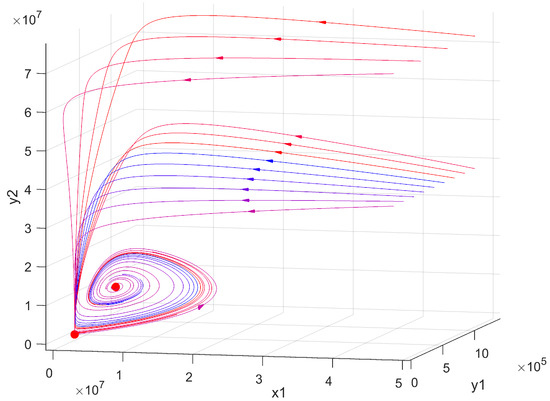
Example 3.

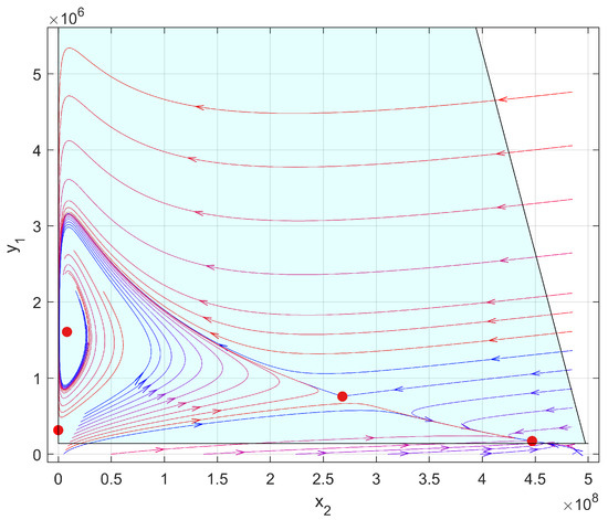
The system ${\mathsf{\Xi }}_1$ with parameters (9) has four EPs:

$$\begin{array}{c}{E}_0=(0;3.16·{10}^5);E_{11}=(4.47·{10}^8;1.73·{10}^5);\\ E_{12}=(2.68·{10}^8;7.59·{10}^5);E_{13}=(8.19·{10}^6;1.608·{10}^6);\end{array}$$

$E_0$ and $E_{12}$ are saddles, $E_{11}$ is a stable node, and $E_{13}$ is a stable focus. The conditions of competitiveness, dissipativity, and conditions of Theorem 8 are not satisfied. A phase portrait of the system is presented in Figure 1.

Figure 1. A phase portrait of the system ${\mathsf{\Xi }}_1$.

7. The System $\mathsf{\Xi }$ on $x_2=0$

In the plane $x_2=0$, the dynamics of the system $\mathsf{\Xi }$ is described by the equations

$$\begin{array}{c}{\dot{x}}_1=a_1{x}_1(1-b{x}_1)-{\mu }_1{x}_1{y}_1-\beta x_1{y}_2,\hfill \\ {\dot{y}}_1=c_1-c_2{y}_1-c_3{x}_1{y}_1+\frac{c_4{x}_1{y}_1}{c_5+x_1},\hfill \\ {\dot{y}}_2=d_1{x}_1{y}_1-d_2{x}_1{y}_2-d_3{y}_2.\hfill \end{array}$$

(31)

This system (we denote it by ${\mathsf{\Xi }}_2$) has the EP $(0,c_1/c_2,0)$ corresponding to the EP $E_0=(0,0,c_1/c_2,0)$ of the system $\mathsf{\Xi }$, as well as up to four inner EPs.

The EP $E_0$ is locally asymptotic stable if $c_1{\mu }_1>a_1{c}_2$. Let us find sufficient conditions of global asymptotic stability of $E_0$.

Theorem 9.

If

$$\frac{c_1{\mu }_1}{a_1}>\frac{c_2}{2}+\frac{c_2^2{c}_3}{4b}+\frac{b}{4c_3}$$

or

$$\frac{c_1{\mu }_1}{a_1}>c_2,b>c_2{c}_3$$

then all trajectories of the system ${\mathsf{\Xi }}_2$ tend to $E_0$.

Proof. 

We take a localizing function $h_7=x_1{y}_1^{-\eta }$ and act like in proof of Theorem 8. □

Example 4.

The system ${\mathsf{\Xi }}_2$ with parameters (9) has two EPs:

$$E_0=(0,3.16·{10}^5,0);E_2=(3.68·{10}^6,5.59·{10}^5,1.064·{10}^7);$$

$E_0$ is a saddle and not stable, $E_2$ is a stable focus. The conditions of Theorem 9 are not satisfied. A phase portrait of the system is presented in Figure 2.

Figure 2. A phase portrait of the system ${\mathsf{\Xi }}_2$.

8. Concluding Remarks

In this article, one cancer model has been analyzed for which the heterogeneity within the tumor for various phenotypic factors is taken into account. This heterogeneity of the model is a consequence of various coefficient values of the equations describing the dynamics of two cancer cell populations, as well as of various terms in these equations. As a result of the analysis of this model, bounds for the ultimate system dynamics are obtained: a polytope $\mathsf{\Pi }$ is constructed in the non-negative orthant, which is positively invariant and attracting, i.e., all trajectories in non-negative orthant tend to this polytope. This cancer system may have a large number of equilibrium points—up to 14, and, namely, in addition to the standard cancer free EP $E_0$, up to three EPs in the invariant plane $x_1=0$, up to four in the invariant plane $x_2=0$, and up to six inner EPs. It is not known if there is a set of biologically reasonable values of parameters under which this entire set of EPs is realized, but these estimates indicate that the behavior of the system can be complex. Further, we studied an important case where extinction of cancer populations is achieved. From a biological point of view, this can be interpreted as a cure for the disease, since in this case the growth of the tumor can be controlled after a certain period of observation. These conditions have been derived in the form of GATE conditions for the cancer free EP $E_0$. It is curious that GATE conditions as well as conditions for the location of $\omega$-limit sets in coordinate planes, do not depend on several model parameters including $\beta$, $d_1$, $d_2$, $d_3$. Further, we described the case when GATE conditions are the best possible. In [7], in the course of computational experiments, typical bifurcations of equilibrium positions were discovered: transcritical, saddle-node (fold), Hopf bifurcation. However, there are areas in the parameter space for which the behavior of the system is relatively simple and reduces to zeroing the variables that describe the dynamics of cancer cells. Information about such regions, in our opinion, will be useful in further analysis of both this model and those close to it.

We hope that this kind of analysis of tumor—immune system interactions may be useful to understand qualitatively some mechanisms underlying the tumor dynamics, allowing a theoretical basis for new studies in order to create new more biologically complete cancer models including multi-phenotypic features, and more efficient treatment protocols.

References

- Fidler, I.J.; Hart, I.R. Biological diversity in metastatic neoplasms: Origins and implications. Science 1982, 217, 998–1003. [Google Scholar] [CrossRef] [PubMed]
- Heppner, G.H.; Miller, F.R. The cellular basis of tumor progression. Int. Rev. Cytol. 1997, 177, 1–56. [Google Scholar]
- Talmadge, J.E.; Wolman, S.R.; Fidler, I.J. Evidence for the clonal origin of spontaneous metastases. Science 1982, 217, 361–363. [Google Scholar] [CrossRef]
- Marusyk, A.; Polyak, K. Tumor heterogeneity: Causes and consequences. Biochim. Biophys. Acta (BBA) Rev. Cancer 2010, 1805, 105–117. [Google Scholar] [CrossRef]
- Marusyk, A.; Almendro, V.; Polyak, K. Intra-tumour heterogeneity: A looking glass for cancer? Nat. Rev. Cancer 2012, 12, 323–334. [Google Scholar] [CrossRef]
- Diaz-Cano, S.J. Tumor heterogeneity: Mechanisms and bases for a reliable application of molecular marker design. Int. J. Mol. Sci. 2012, 13, 1951–2011. [Google Scholar] [CrossRef]
- Alvarez, R.F.; Barbuto, J.A.; Venegeroles, R. A nonlinear mathematical model of cell-mediated immune response for tumor phenotypic heterogeneity. J. Theor. Biol. 2019, 471, 42–50. [Google Scholar] [CrossRef]
- Bayer, P.; Brown, J.S.; Stankova, K. A two-phenotype model of immune evasion by cancer cells. J. Theor. Biol. 2018, 455, 191–204. [Google Scholar] [CrossRef]
- Harris, L.A.; Beik, S.; Ozawa, P.M.; Jimenez, L.; Weaver, A. Modeling heterogeneous tumor growth dynamics and cell–cell interactions at single-cell and cell-population resolution. Curr. Opin. Syst. Biol. 2019, 17, 24–34. [Google Scholar] [CrossRef]
- Shu, Y.; Huang, J.; Dong, Y.; Takeuchi, Y. Mathematical modeling and bifurcation analysis of pro- and anti-tumor macrophages. Appl. Math. Model. 2020, 88, 758–773. [Google Scholar] [CrossRef]
- Kuznetsov, V.A.; Makalkin, I.A.; Taylor, M.A.; Perelson, A.S. Nonlinear dynamics of immunogenic tumors: Parameter estimation and global bifurcation analysis. Bull. Math. Biol. 1994, 56, 295–321. [Google Scholar] [CrossRef] [PubMed]
- Kirschner, D.; Panetta, J. Modelling immunotherapy of the tumor-immune interaction. J. Math. Biol. 1998, 37, 235–252. [Google Scholar] [CrossRef] [PubMed]
- Owen, M.; Sherratt, J. Modelling the macrophage invasion of tumors: Effects on growth and composition. Math. Med. Biol. 1998, 15, 165–185. [Google Scholar] [CrossRef]
- de Pillis, L.G.; Radunskaya, A. The dynamics of an optimally controlled tumor model: A case study. Math. Comput. Model. 2003, 37, 1221–1244. [Google Scholar] [CrossRef]
- Eftimie, R.; Bramson, J.L.; Earn, D.J.D. Interactions between the immune system and cancer: A brief review of non-spatial mathematical models. Bull. Math. Biol. 2011, 73, 2–32. [Google Scholar] [CrossRef]
- Yin, A.; Moes, D.J.A.; van Hasselt, J.G.; Swen, J.J.; Guchelaar, H.J. A review of mathematical models for tumor dynamics and treatment resistance evolution of solid tumors. CPT Pharmacomet. Syst. Pharmacol. 2019, 8, 720–737. [Google Scholar] [CrossRef]
- Krishchenko, A.P. Localization of invariant compact sets of dynamical systems. Differ. Equ. 2005, 41, 1669–1676. [Google Scholar] [CrossRef]
- Krishchenko, A.P.; Starkov, K.E. Localization of compact invariant sets of the Lorenz system. Phys. Lett. A 2006, 353, 383–388. [Google Scholar] [CrossRef]
- Hirsch, M.W. Systems of differential equations that are competitive or cooperative I: Limit sets. SIAM J. Math. Anal. 1982, 13, 167–179. [Google Scholar] [CrossRef]
- Khalil, H.K. Nonlinear Systems, 3rd ed.; Printice Hall: Upper Saddle River, NJ, USA, 2002. [Google Scholar]
- Ye, Y.; Cai, S.L. Theory of Limit Cycles; American Mathematical Soc.: Providence, RI, USA, 1986. [Google Scholar]
- Starkov, K.E.; Bunimovich-Mendrazitsky, S. Dynamical properties and tumor clearance conditions for a nine-dimensional model of bladder cancer immunotherapy. Math. Biosci. Eng. 2016, 13, 1059–1075. [Google Scholar] [CrossRef]
- Starkov, K.E.; Kanatnikov, A.N. Cancer cell eradication in a 6D metastatic tumor model with time delay. Commun. Nonlin. Sci. Numer. Simul. 2023, 120, 107164. [Google Scholar] [CrossRef]
- Abernathy, K.; Abernathy, Z.; Dougherty-Bliss, R.; Mayer, C.; Whiteside, H. Global dynamics of a cancer stem cell treatment model. Int. J. Dynam. Syst. Differ. Equ. 2019, 9, 176–186. [Google Scholar] [CrossRef]
- Abernathy, K.; Abernathy, Z.; Baxter, A.; Stevens, M. Global dynamics of a breast cancer competition model. Differ. Equ. Dyn. Syst. 2020, 28, 791–805. [Google Scholar] [CrossRef] [PubMed]
- Liu, P.; Liu, X. Dynamics of a tumor-immune model considering targeted chemotherapy. Chaos Solitons Fractals 2017, 98, 7–13. [Google Scholar] [CrossRef]
Disclaimer/Publisher’s Note: The statements, opinions and data contained in all publications are solely those of the individual author(s) and contributor(s) and not of MDPI and/or the editor(s). MDPI and/or the editor(s) disclaim responsibility for any injury to people or property resulting from any ideas, methods, instructions or products referred to in the content. |
© 2023 by the authors. Licensee MDPI, Basel, Switzerland. This article is an open access article distributed under the terms and conditions of the Creative Commons Attribution (CC BY) license (https://creativecommons.org/licenses/by/4.0/).