Abstract
We consider a mechanical system that is comprised of three parts: a rigid outer shell with a spherical cavity, a spherical core inside this cavity, and an intermediate layer of liquid between the core and the shell. Such a model provides an adequate description of the behavior of a wide variety of celestial bodies. The centers of the inner and outer liquid’s spherical boundaries are assumed to coincide. Assuming that the viscosity of the liquid is high, we obtained an approximate solution to the Navier–Stokes equations that describes a so called creeping flow of the liquid, which sets on after all transient processes die out. We note that the effect of the liquid on the rotational motion of the system can be modeled as a special torque acting upon the system with “solidified” fluid.
MSC:
74F10; 76D05; 76U05; 76M45
1. Introduction
It is customary to model a celestial object as a three-component structure comprised of an inner core, an intermediate layer of liquid, and an outer solid shell [1,2,3,4,5,6,7,8]. We will deal with the simplest, but fairly common version of such an approach, which does not take into account that in reality the interfaces between liquid and solid components represent a mushy transition zone [9,10]. The mass proportion of each component strongly depends on the object’s type. For example, the core of an Earth-like planet is considerably smaller than the outer shell (mantle) (Figure 1a). At the same time, the icy crust, covering the hypothetical subsurface oceans of some satellites of Jupiter and Saturn, is relatively thin as compared to the satellites’ radii (Figure 1b) [11]. Studying the dynamics of the multi-component object it is convenient to fix a coordinate frame to the most dominant component (either outer shell or inner core) and investigate the behavior of the other components relative to this frame.
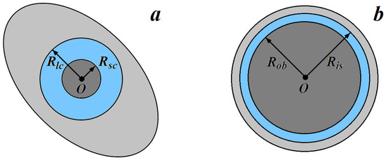
Figure 1.
Celestial objects modeled as multi-shell structures: (a) “planet” (small inner core), (b) “icy satellite” with thin outer layer of ice, covering the subsurface ocean. In the case of a “planet,” the radii of the inner and outer boundaries of the liquid layer are denoted by and ; in the case of an icy satellite, they are denoted by and , respectively. The visible contours of a body can have any shape; the only thing that matters is that the center of mass of the outer component coincides with the center of the cavity.
In the theory of the rotating mass of liquid, the key role plays Ekman number [12], which reads
Here, is the characteristic angular velocity of system’s components, is the characteristic size (e.g., the radius of the outer boundary of the liquid layer), is the density of the liquid, and is the liquid’s viscosity.
If , the flow of the liquid within the layer is known to be Stokesian or creeping [13]. In this case, the approximate relations for the liquid’s velocities can be obtained from the Navier–Stokes equations with the relative-acceleration terms neglected. Stokes flow in the gap between two concentric spheres has been considered by many experts. However, in the best part of the studies the motion of the bounding surfaces was assumed to be known, and the effect the liquid invokes on their dynamics was not studied (e.g., see [14,15]).
In [16], F.L. Chernousko showed that when the analysis of the dynamics of a body containing a cavity filled with liquid can be simplified: the liquid in the cavity is considered “solidified”, and the liquid’s effect on the body is modeled as an additional torque applied to the body. Various aspects of the Chernousko approach are discussed in [17,18].
In the current paper, we show that in the case , a similar approach can be used for analyzing the rotation of celestial objects containing liquid layers. A useful byproduct of such an approach is an approximate formula for the velocity field of the liquid particles.
As far as we know, there are no multi-component celestial bodies with . Therefore, at least at present, our results seem to have only a peripheral relationship to the dynamics of actual astrophysical objects. At the same time, our results may be used, for example, for testing software that simulates the dynamics of such objects when it is important to be able to compare numerical results with a known analytical solution, regardless of whether this solution represents a real phenomena [19].
The paper is organized as follows. In Section 2, the governing equations for a three-component system mantle+liquid+core are presented. An approximate formula for the liquid velocity field after Stokes (creeping) flow sets in is obtained in Section 3. A condition of “dynamical agreement” between the motion of the core and the motion of the liquid near the core’s surface is presented in Section 4. This condition helps to establish all of the parameters of the liquid flow. Section 5 discusses some aspects of this flow. In Section 6, the approximate relations describing the regular precession of the mantle relative to the core are given. Some issues associated with the introduction of the additional torque that replicates the action of the liquid (the Chernousko model) are covered in Section 7. Modifications to the formulas for the liquid velocity to suit the case where the thin outer shell moves relative to the massive core are discussed in Section 8. A brief outline of the results obtained is presented in Section 9.
2. Equations of Motion of a “Planet”
We assume that the external forces and torques applied to the system allow for a motion in the course of which the center of mass of the outer shell (referred to further as mantle) coincides with the center of mass of the inner core. Such a regime (at least approximately) occurs when a “planet” orbits a star. Under this assumption, the motion of the core relative to a mantle-fixed frame is a rotation with angular velocity . For simplicity, we assume that the motion of the centers of mass is known (i.e., and are known functions of time). Relative to the frame , the motion of the liquid is governed by the Navier–Stokes equations
Here, is the liquid velocity, is the pressure in the liquid layer, is the potential of the gravity attraction forces exerted on the liquid particles, is the angular velocity of the frame , and is the liquid’s kinematic viscosity. The velocity satisfies the standard incompressibility condition
and the kinematic relations
where and stand for the radius of the cavity and the core, respectively.
Within the core, the distribution of the matter’s density is assumed to be spherically symmetric. In the frame , the evolution of its rotational speed is governed by the equation
Here, is the friction torque that the liquid exerts on the core. To find , we integrate the tangential stress components over the core’s surface , that is,
Here, T is the stress tensor and is the unit outward normal to the surface of the core.
The total angular momentum relative to the center of mass can be decomposed as
Here, is the angular momentum of the “solidified” planet in which the liquid and the inner core are fixed relative to the mantle; the internal momentum of the liquid can be written as ; the attitude momentum of the core reads ; and , where stands for the tensor of inertia of the “solidified” planet. Let be the net external torque applied to the system; then, the time evolution of the total angular momentum is described by the Euler equation
The governing equations should be augmented with kinematic relations of the form
where the parameters quantify the orientation of the mantle-fixed frame (e.g., the Euler angles).
Hereafter, the units of mass, length, and time are assumed to be so chosen that and therefore
3. Stokes Flow in the Liquid Layer
If after an initial transient process, the flow in the cavity becomes creeping flow [13]. Omitting the inertial terms in (1) yields the following equation governing the creeping flow:
where the velocity satisfies the incompressibility condition (2) and the kinematic relations (3) and (4).
We seek a solution to (8) of the form
which upon substitution into (8) provides the following equation in the function
The velocity field satisfies the boundary condition provided that
To meet the boundary condition (3), the rotation of the inner core and the velocity (9) must agree kinematically, that is,
Moreover, Equation (5) implies a certain “dynamical” agreement between the motion of the liquid and the motion of the inner core. In Section 4, we will derive the value of for which (12) provides an approximate solution to (5), thereby revealing the dynamics of all of the system’s components. For simplicity, put
By symmetry, it is quite natural to assume that the solution to the boundary-value problems (10)–(12) and (14) lies among functions that depend solely on . For such functions, this problem reduces to the boundary-value problem for the third-order ODE
of the form
The solution to the boundary-value problems (15) and (16) looks like
where the constants satisfy the linear relations
It is straightforward to obtain
and
4. “Dynamical” Agreement between the Motion of the Inner Core and the Liquid
From Equation (5), it follows that after the creeping flow onset one has
To obtain , one should calculate the integral (6). Following [14], introduce spherical coordinates whose polar axis is aligned with . The velocity components of a liquid particle are
The force per unit area of the surface of the inner core can be determined with the help of the -component of the stress tensor T
Integrating over the sphere’s surface yields
where is the central moment of inertia of the cavity of radius filled with liquid with density .
Equating (18) and (19) we obtain
With this expression for at our disposal, it is easy to find that
The graph of is given in Figure 2. It can be easily checked that when , which is quite natural since usually the inner core is more dense than the liquid.
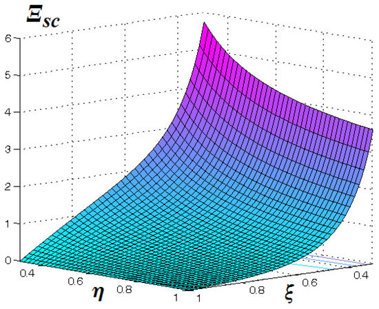
Figure 2.
The graph of the function . The argument characterizes the ratio of the radii of the inner and outer boundaries of the liquid layer, and the argument represents the ratio of the densities of the liquid and the substance of the inner core (assumed homogeneous).
5. Common Properties of the Flow in the Liquid Layer
Using (9), (17) and (20), it is possible to draw the lines of constant velocity magnitude in a plane through the axis of relative rotation of the inner core (Figure 3). Obviously, the magnitude acquires its maximum in the ”equatorial” plane, which is perpendicular to the relative angular velocity of the core and passes through its center.
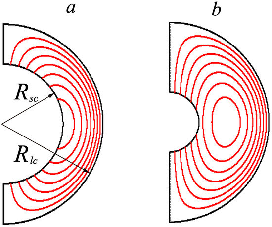
Figure 3.
Velocity level lines in a plane through the instantaneous axis of relative rotation of the inner core (which is also the flow’s axis of symmetry) when : (a) (the velocity of the liquid reaches its maximum on the surface of the inner core), (b) (the maximal velocity of the flow is attained inside the layer).
The most trivial distribution of the velocity magnitude occurs when
Assuming that the core is uniform in density, Equation (21) implies that its density is equal to the density of the ambient liquid. So, if (21) is fulfilled, then in the equatorial plane
Thus, if the maximum of the magnitude is reached on the surface of the inner core, whereas for the maximum occurs at .
6. Motion of the Core Relative to the Mantle
The attitude dynamics of the core is governed by Equation (5). Let us examine the dynamics in greater detail assuming that the mantle is a dynamically symmetric rigid body that is in a precession motion with parameters and ; as usual, is the precession angular velocity, stands for the intrinsic angular velocity, and is the angle between the mantle’s axis of symmetry and the precession axis. Suppose that the -axis of the mantle-fixed frame is aligned with the symmetry axis; then, in this frame the angular velocity of the mantle and the relative angular velocity of the core (up to an inessential time shift) can be written as
Let three orthogonal unit vectors be fixed to the core. The kinematic equations
admit a solution
This solution can be characterized as the core “swaying” with zero secular drift with respect to the mantle. The other solutions to (23) can be obtained from (24) by the action of the rotation group.
Remark. The secular drift of the core still can occur in the course of the mantle’s moderate despinning or acceleration. For example, suppose and the mantle gradually decelerates; then, with respect to the frame , the inner core rotates with angular velocity in the direction opposite the vector of angular acceleration. In a sense, this mimics the superrotation of Earth’s inner core [20]. However, the current concept is that quantitatively reliable estimates of the superrotation can only be obtained with due regard for dynamo effects and turbulent convection within the liquid layer.
7. Chernousko’s Approach to Modelling Rotational Motion of the System
The total attitude angular momentum reads
The integral evaluates as follows:
Here,
From (12) and (26), it follows that
The approach proposed by F.L. Chernousko to modeling the dynamics of a rigid body with a cavity entirely filled with a highly viscous liquid is as follows: the liquid is assumed to be frozen or “solidified”; the influence of the liquid is then represented as a special torque acting upon the body with solidified liquid [16]. In the context of this approach, the Euler equations can be rewritten as
where
Suppose that the derivatives and in (28) are found for the “zero approximation” model, that is, when the “planet” is assumed to be a one-piece uniform rigid body; then, Equation (27), together with the kinematic relations (7), forms a finite-dimensional dynamical system that governs our originally infinite-dimensional system. Such models (obtained within Chernousko’s approach) are as accurate as during time [17,18].
8. Simple Dynamical Model of an “Icy Satellite” with Subsurface Ocean
We now turn to the dynamics of the so-called membrane worlds encountered in the satellite systems of the giant planets [11]. Consider a satellite in the shape of a sphere of radius about which a thin icy shell (crust) is floating on a liquid layer (subsurface ocean). The inner radius of the icy crust will be further denoted as .
By a similar argument as in Section 3 and Section 4, it can be shown that the creeping flow of the ocean is described by formula (9), in which
Here, is the moment of inertia of the icy crust, and is the moment of inertia of a ball of radius , whose density is equal to the density of the liquid; both moments are about an axis through the center of mass.
Lines of equal velocity magnitude in a plane through the axis of relative rotation of the crust are shown in Figure 4.
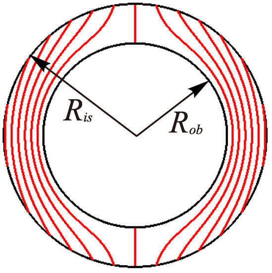
Figure 4.
Distribution of velocities in the ocean: lines of equal velocity magnitude in a plane through the instantaneous axis of relative rotation of the icy crust (which is the flow’s axis of symmetry) for .
The relative angular velocity of the crust is , where
It is easy to verify that for , the following relation holds
This means that for a relatively shallow ocean (), the coefficient is positive. Thus, in this case when a satellite moves with angular acceleration (or deceleration), the icy crust will drift relative to the core with angular velocity in the direction opposite the vector The drift of the icy crust of some giant-planet satellites is discussed in, for example, [21,22]. Since for these objects the condition does not hold, our results can hardly help to obtain new observationally confirmed features of their behavior.
9. Conclusions
We studied the motion of the liquid in the layer between two concentric spherical surfaces. In the case where the motion of one surface is solely determined by the moment of the tangential stress, an approximate expression for the Stokes flow of the liquid is derived. Using this expression, we identified an important class of motions of the three-component system mantle+liquid+core, namely, where the motion of one of the bodies and the liquid are subordinate to the motion imparted by the other body. We showed that such a subordination can be used to obtain a finite dimensional model of the system (the effect of intrinsic motion of liquid particles is modelled as a torque applied to “solidified” system [16]).
Although our study was inspired by real models used to investigate the dynamics of astrophysical objects, our main results were obtained under assumptions that can hardly be met within these models’ framework. Nevertheless, it is worth noting that in the classical problem of describing a creeping flow between two concentric spherical surfaces, we have found a new class of approximate solutions that is valuable in its own right. For example, such solutions can be useful for testing special flow analysis software (as mentioned in the Introduction).
Future research may include the application of perturbation theory for obtaining similar results when the surfaces bounding the flow are not spherical [23,24]. Additionally, our approach may find its application in the study of porous bodies floating within liquid-filled cavities [25,26].
Author Contributions
Conceptualization, V.S. and S.R.; Investigation, V.S. and S.R. All authors have read and agreed to the published version of the manuscript.
Funding
V.V. Sidorenko acknowledges the financial support of his participation in this study by the Scientific and Educational Mathematical Center “Sofia Kovalevskaya Northwestern Center for Mathematical Research” (contract 075-02-2022-891 from 31 January 2022). The work of S.M. Ramodanov is supported by RFBR grant 20-01-00312A “Resonance effects and chaos in the three-body problem”.
Data Availability Statement
Not applicable.
Acknowledgments
The authors thank the anonymous reviewers for helpful comments.
Conflicts of Interest
The authors declare that they have no known competing financial interests or personal relationships that could have appeared to influence the work reported in this paper.
References
- Busse, F.H. On the free oscillations of the Earth’s inner core. J. Geophys. Res. 1974, 79, 753–757. [Google Scholar] [CrossRef]
- Dehant, V.; Van Hoolst, N.; de Veres, O.; Greff-Lefftz, M.; Legros, H.; Defraigne, P. Can a solid inner core of Mars be detected from observations of polar motion and nutations of Mars? J. Geophys. Res. 2003, 108, 1.1–1.12. [Google Scholar] [CrossRef]
- Getino, J.; Farto, J.M.; Ferrandiz, J.M. Obtaining the free frequencies of the non-rigid Earth. Celest. Mech. Dyn. Astr. 1999, 71, 95–108. [Google Scholar] [CrossRef]
- Grinfeld, P.; Wisdom, J. Motion of the mantle in the translational modes of the Earth and Mercury. Phys. Earth Planet. Inter. 2005, 151, 77–87. [Google Scholar] [CrossRef]
- Hussmann, H.; Sohl, F.; Spohn, T. Subsurface oceans and deep interiors of medium-sized outer planet satellites and large transneptunian objects. Icarus 2006, 185, 258–273. [Google Scholar] [CrossRef]
- Kitiashvili, I.; Gusev, A. Inner core wobble and free core nutation of pulsar PSR B1828-11. Adv. Space Res. 2003, 42, 1391–1397. [Google Scholar] [CrossRef]
- Nimmo, F.; Rappalardo, R.T. Ocean worlds in outer Solar system. J. Geophys. Res. Planets 2016, 121, 1378–1399. [Google Scholar] [CrossRef]
- Shematovich, V.I. Ocean worlds in the outer regions of the Solar system (review). Sol. Syst. Res. 2018, 52, 371–381. [Google Scholar] [CrossRef]
- Loper, D.E.; Fearn, D.R. A seismic model of a pertial molten inner core. J. Geophys. Res. 1983, 88, 1235–1242. [Google Scholar] [CrossRef]
- Peng, Z.R. Effects of a mushy transition zone at the inner core boundary on the Slicher modes. Geophys. J. Int. 1997, 131, 607–617. [Google Scholar] [CrossRef]
- Beuthe, M. Tidal Love numbers of membrane worlds: Europa, Titan, and Co. Icarus 2016, 258, 239–266. [Google Scholar] [CrossRef]
- Greenspan, H.P. The Theory of Rotating Fluids; Cambridge University Press: Cambridge, UK, 1968. [Google Scholar]
- Happel, J.; Brenner, H. Low Reynolds Number Hydrodynamics: With Special Applications to Particulate Media; Prentice-Hall: Englewood Cliffs, NJ, USA, 1965. [Google Scholar]
- Landau, L.D.; Lifshitz, E.M. Fluid Mechanics, 2nd ed.; Pergamon Press: Oxford, UK, 1987. [Google Scholar]
- Shankar, P. Exact solutions for Stokes flow in and around a sphere and between concentric spheres. J. Fluid Mech. 2009, 631, 363–373. [Google Scholar] [CrossRef]
- Chernousko, F.L. Motion of a Rigid Body with Cavities Containing a Viscous Fluid; NASA Technical Translations; Computing Centre of the USSR Academy of Sciences: Moscow, Russia, 1972. [Google Scholar]
- Bogatyrev, S.V. Slow motions in problems of the dynamics of a solid with a cavity filled with a viscous liquid. J. Applied Math. Mech. 1994, 58, 849–855. [Google Scholar] [CrossRef]
- Ramodanov, S.M.; Sidorenko, V.V. Dynamics of a rigid body with an ellipsoidal cavity filled with viscous fluid. Int. J. Non-Linear Mech. 2017, 95, 42–46. [Google Scholar] [CrossRef]
- Child, A.; Hollerbach, R.; Kersale, E. Axisymmetric pulse train solutions in narrow-gap spherical Couette flow. Phys. D Nonlinear Phenom. 2017, 348, 54–59. [Google Scholar] [CrossRef][Green Version]
- Song, X.; Richards, R.G. Seismological evidence for differential rotation of the Earth’s inner core. Nature 1996, 382, 221–224. [Google Scholar] [CrossRef]
- Goldreich, P.M.; Mitchell, J.L. Elastic ice shells of synchronous moons. Implications for cracks on Europa and non-synchronous rotation of Titan. Icarus 2010, 209, 631–638. [Google Scholar] [CrossRef][Green Version]
- Patthoff, D.A.; Kattenhorn, S.A.; Cooper, C.M. Implications of nonsynchronous rotation on the deformational history and ice shell properties in the south polar terrain of Enceladus. Icarus 2019, 321, 445–457. [Google Scholar] [CrossRef]
- Denisov, G.G.; Novikov, V.V. On fluid flow between rotating surfaces. J. Appl. Mech. Tech. Phys. 2011, 52, 31–36. [Google Scholar] [CrossRef]
- Prasad, M.K.; Kaur, M.; Srinivasacharya, D. Slow steady rotation of an approximate sphere in an approximate spherical container with slip surfaces. Int. J. Appl. Comput. Math. 2017, 3, 987–999. [Google Scholar] [CrossRef]
- Keh, H.J.; Lu, Y.S. Creeping motion of a porous spherical shell in concentric spherical cavity. J. Fluid. Struct. 2005, 20, 735–747. [Google Scholar] [CrossRef]
- Verma, V.K.; Verma, H. Motion of a porous spherical shell in a spherical container. Spec. Top. Rev. Porous Media 2019, 10, 525–537. [Google Scholar] [CrossRef]
Disclaimer/Publisher’s Note: The statements, opinions and data contained in all publications are solely those of the individual author(s) and contributor(s) and not of MDPI and/or the editor(s). MDPI and/or the editor(s) disclaim responsibility for any injury to people or property resulting from any ideas, methods, instructions or products referred to in the content. |
© 2023 by the authors. Licensee MDPI, Basel, Switzerland. This article is an open access article distributed under the terms and conditions of the Creative Commons Attribution (CC BY) license (https://creativecommons.org/licenses/by/4.0/).