Article

Robustness of the -Rule for an Unreliable Single-Server Two-Class Queueing System with Constant Retrial Rates

1
Institute for Stochastics, Johannes Kepler University Linz, 4040 Linz, Austria
2
Scientific and Production Company “INSET”, Moscow 129085, Russia
3
Department of Informatics and Networks, Faculty of Informatics, University of Debrecen, 4032 Debrecen, Hungary
*
Author to whom correspondence should be addressed.
Mathematics 2023, 11(18), 4002; https://doi.org/10.3390/math11184002
Submission received: 9 August 2023 / Revised: 18 September 2023 / Accepted: 19 September 2023 / Published: 20 September 2023

Abstract

:
We study the robustness of the c μ -rule for the optimal allocation of a resource consisting of one unreliable server to parallel queues with two different classes of customers. The customers in queues can be served with respect to a FIFO retrial discipline, when the customers at the heads of queues repeatedly try to occupy the server at a random time. It is proved that for scheduling problems in the system without arrivals, the c μ -rule minimizes the total average cost. For the system with arrivals, it is difficult directly to prove the optimality of the same policy with explicit relations. We derived for an infinite-buffer model a static control policy that also prescribes the service for certain values of system parameters exclusively for the class-i customers if both of the queues are not empty, with the aim to minimize the average cost per unit of time. It is also shown that in a finite buffer case, the c μ -rule fails.

1. Introduction

The modeling and analysis of telecommunications and computer systems is now inconceivable without the various tasks associated with resource allocation and formulated in the framework of queueing theory. One such classic problem is to allocate a server to multiple parallel queues with the most-studied objective of minimizing the average cost per unit of time. There is a great diversity in the application of such controlled systems, for example, the task of scheduling a processor in multilevel programming, the transmission of different types of packages in a telecommunications network, or a machine tool that processes different types of work pieces. It was shown that for many systems with such kinds of resource allocation problems, the allocation policy in the form of the c μ -rule is optimal. In the literature, this rule is also known as Smith’s rule or weighted shortest processing time. According to this rule, the waiting class-i customer from a non-empty queue is allocated to the server if it has a maximal weight of the form c i μ i , where c i is a holding cost per unit of time the customer is in the queue or at the server and μ i is an overall service rate of the class-i customer. The c μ -rule is a very attractive policy since it is a static one and requires only the information regarding whether a certain queue is empty or not. Obviously, to apply such a policy, the values c i and μ i must be known, which unfortunately is not always the case, especially for the overall service intensity.
The optimality of the c μ -rule for ordinary multi-class single-server queues in different settings was proved; see e.g., [1,2]. The result was extended in [3] for the discrete-time dynamic scheduling problems of three types of general G / G / 1 queue with K classes of customers. A detailed review of works on the c μ -rule can also be found in M.Sc. thesis [4]. In [5], the authors analyzed the c μ -rule for queueing models with non-linear costs. The optimality of this rule for discrete-time queueing models with a general distributed inter-arrival time and geometrically distributed service time was established in [6]. The concept of a generalized c μ -rule was proposed in [5], where it was shown that this rule is asymptotically optimal for non-decreasing convex delay costs. A classic scheduling problem with a single resource shared by two competing queues was considered in [7] in the context of the stochastic flow model, where it was shown that the c μ -rule is optimal. The non-preemptive assignment of a single server to two infinite-capacity retrial queues was analyzed in [8], where the c μ -rule was optimal for a scheduling problem in a system without arrivals. The authors in [9] considered the learning-based variants of the c μ -rule where the service rates μ are unknown.
Most often, systems with retrials assume that customers make repeated attempts independently of each other to occupy the server after a random time. Such systems are referred to as the systems with level-dependent retrial rates or with classical retrial policies. A detailed review of such systems can be found, e.g., in [10,11]. Nevertheless, in computer networks, the conditions according to the classical retrial policy are not always fulfilled. Sometimes, there is a situation when the customer at the head of the queue in the ordinary queueing system has no information about the state of the server and retries for service after a random time. There may also be situations where the server needs to check whether a transmission facility is available, or it may need time to find a specified customer. In these tasks, the retrial intensity is independent of the number of customers in the orbit; that is, a constant retry policy is quite appropriate to describe the behavior of customers when retries occur. The constant retrial policy was introduced in [12], where it was assumed that only the customer at the head of the queue can request service after an exponentially distributed retrial time. The single-class queueing systems with constant retrial rates and different options were analyzed intensively, e.g., in [13,14,15] and other papers. The uncontrolled analog of a two-class queueing system has also been investigated by a number of authors. For example, in [16], the authors studied a two-class system with a single exponential service requirement and constant retrial policy. The regenerative approach was used there to derive a set of necessary stability conditions of such a system. However, in this system, no dynamic control was assumed to be possible. The generating function of the stationary distribution of the number of orbiting customers at service completion epochs was obtained in [17]. Among recent works on parallel queues with constant retrial policies, we can mention a study proposed in [18], where stability conditions for both an uncontrolled system and a c μ -controlled system were derived.
This paper deals with a controllable unreliable single-server two-class queueing system with constant retrial rates. The optimal allocation problem for this queueing model with retrial and reliability attributes is a new one, and our research aims are different from those previously studied. The emphasis of the paper is on answering the question of how robust the c μ -rule is as an optimal allocation policy in the queueing system under study. The queueing system is studied without and with arrivals. In the first case, explicit relations of the c μ -rule can be derived. In the second case, the relations for the optimality of a variant of the c μ -rule were obtained for the model with a certain constraint on the arrival process.
In Section 2, the queueing model is described. The main results, including the analysis of the optimal allocation policy and some numerical experiments, are presented in Section 3.

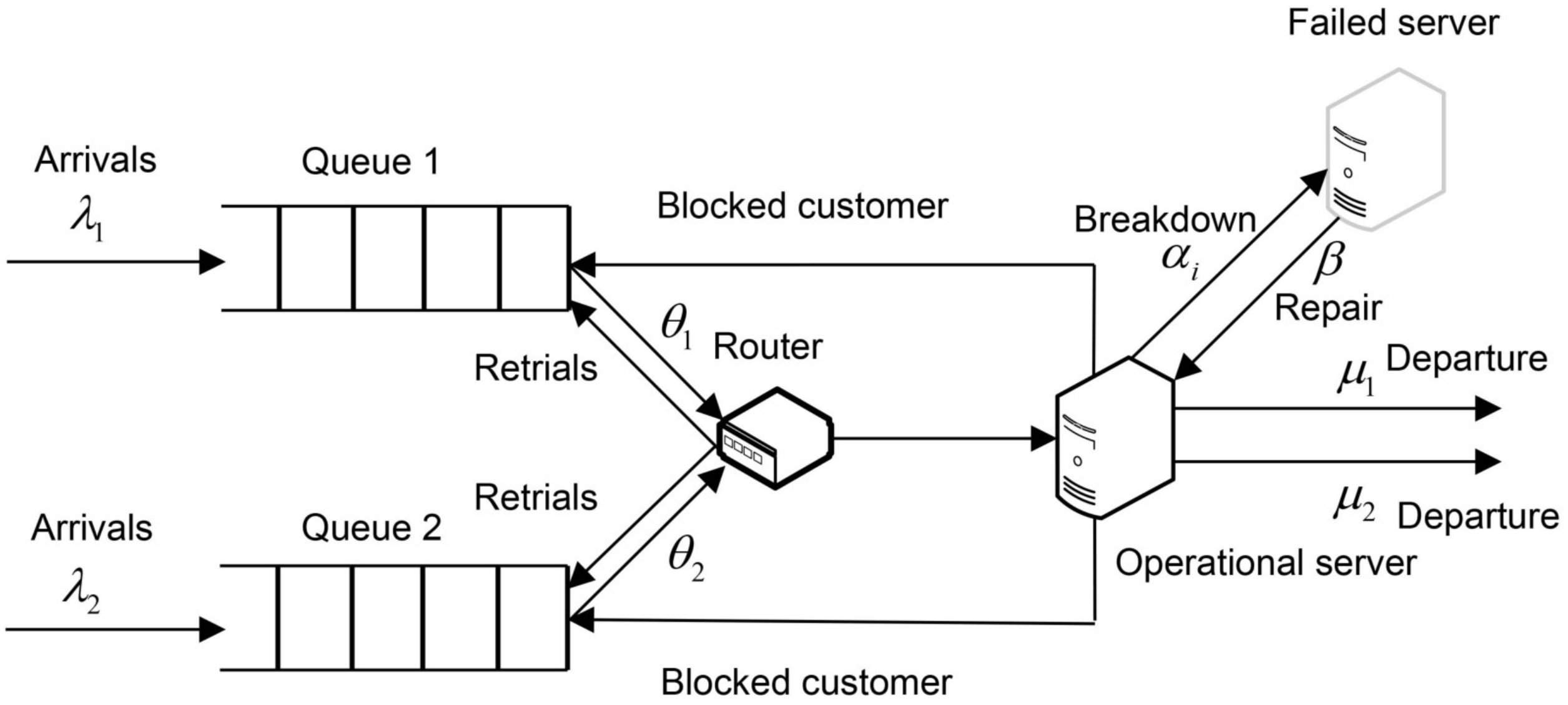
2. Model Description

We analyze the Markovian single-server queueing system servicing two classes of customers, as illustrated in Figure 1. The customers of each class i = 1 , 2 arrive at the system according to a Poisson stream with a rate λ i . Independently of the state of the server, the class-i customers join the corresponding waiting line or queue with infinite capacity N i = upon arrival. The service of customers from the queue occurs according to a FIFO retrial discipline; i.e., the customer waiting at the head of the queue retries to occupy the server in exponentially distributed time with a rate θ i . The service rate of the ith class customer is μ i . The server during a service process of the ith-class customer can fail in exponentially distributed time with a rate α i . In this case, the customer leaves the service area and joins the head of its queue again. In the failed state, the server can be repaired in exponentially distributed time with a rate β . All types of time intervals are assumed to be mutually independent. At moments of retrial arrival, the idle server may accept the customer of a certain class who attempts to occupy the server or can deny the service. The system performance is described by the steady state average cost, which is of the form
g f = c 1 L 1 f + c 2 L 2 f ,
where L i f is the average number of the ith-class customers present in the system, given the allocation policy is f and c i is the holding cost per unit of time the ith-class customer spends in the system. The objective of the present analysis is to provide how robust a static policy f is, defined as a c μ -rule for the system under study by minimizing the average cost per unit of time (1).
Denote by Q i ( t ) the number of ith-class customers in the system at time t and by D ( t ) the state of the server at time t, which is defined as follows:
D ( t ) = 0 the server is idle , 1 the server services the 1 st class customer , 2 the server services the 2 nd class customer , 3 the server is failed .
Consider the three-dimensional continuous-time Markov chain
{ X ( t ) } t 0 = { Q 1 ( t ) , Q 2 ( t ) , D ( t ) } t 0 ,
with a state space
E = { x = ( q 1 , q 2 , d ) : q 1 , q 2 N 0 , d { 0 , 1 , 2 , 3 } }
and policy-dependent infinitesimal matrix Λ f = [ λ x y f ] with components for x y ,
λ x y f = λ i y = x + e i , μ i y = x i e 3 , d ( x ) = i , θ i y = x e i + i e 3 , d ( x ) = 0 , f ( x ) = i , α i y = x + e i i e 3 , d ( x ) = i , β y = x 3 e 3 , 0 otherwise ,
where e i stands for a vector of dimension 3 with 1 in the ith position, i = 1 , 2 , 3 , and 0 elsewhere. Here, f is a control policy which prescribes the allocation of the ith-class customer to the server at the moments of retrial arrival. The set of admissible control actions is defined by A = { 1 , 2 } , where f ( x ) = i A means that upon retrial arrival in state x, the ith-class customer must be accepted for service. The sets of admissible control actions in state x are denoted by A ( x ) A , where A ( x ) = A for x = ( q 1 , q 2 , 0 ) , q 1 , q 2 1 , A ( x ) = 1 for x = ( q 1 , 0 , 0 ) and A ( x ) = 2 for x = ( 0 , q 2 , 0 ) . It is assumed that the stability condition is fulfilled. According to a general result for the M / G / 1 system with parallel queues, see, e.g., [2]; the system is stable if the total load ρ = ρ 1 + ρ 2 < 1 , where ρ i is the load of the class-i queue. The value ρ i can be obtained if we treat the class-i queue as an independent single-server queueing system with parameters λ i , μ i , θ i , α i , and β . The corresponding continuous-time Markov-chain is then a quasi-birth-and-death (QBD) process with a three-diagonal block infinitesimal matrix:
Q = B 0 B 1 0 0 A 2 A 1 A 0 0 0 A 2 A 1 A 0 0 0 A 2 A 1 , where B 0 = λ i 0 0 μ i ( λ i + μ i + α i ) 0 0 0 1 , B 1 = λ i 0 0 0 λ i α i 0 0 0 , A 1 = ( λ i + θ i ) 0 0 μ i ( λ i + μ i + α i ) 0 β 0 ( λ i + β ) , , A 0 = λ i 0 0 0 λ i α i 0 0 λ i , A 2 = 0 θ i 0 0 0 0 0 0 0 .
According to a matrix-analytic approach for QBD-processes [19], the queue i is stable if the following inequality holds:
p A 2 e > p A 0 e , e = ( 1 , 1 , 1 ) .
where p = ( p 1 , p 2 , p 3 ) is a stationary distribution for the infinitesimal transition matrix
A = A 0 + A 1 + A 2 = θ i θ i 0 μ i ( α i + μ i ) α i β 0 β
which satisfies the system p A = 0 and p e = 1 . The solution of the system is given by
p 1 = ( α i + μ i ) β C , p 2 = β θ i C , p 3 = α θ i C ,
where C = α i ( β + θ i ) + β ( μ i + θ i ) . By substituting the solution (5) into (4) we obtain
ρ i = λ i C β i μ i θ i = λ i α i + μ i μ i θ i θ i β α i + β α i + μ i + 1 < 1 .
and the stability condition is then defined as
i = 1 2 λ i α i + μ i μ i θ i θ i β α i + β α i + μ i + 1 < 1 .
Below, we present the main results of this paper obtained for a system with two classes of customers. However, these results can also be generalized to the case of an arbitrary number of classes.

3. Optimal Allocation Problem

Consider first a classic scheduling problem for the allocation of customers in the system without arrivals, i.e., when λ 1 = λ 2 = 0 , in which the customers are queued. The waiting customers must be served in such a way that the overall average cost is minimized. It is assumed that the allocation policy f ( q 1 , 0 , 0 ) = 1 and f ( 0 , q 2 , 0 ) = 2 for q 1 , q 2 1 . Here, we have a classical scheduling problem.
Proposition 1.
In state x = ( q 1 , q 2 , 0 ) , the optimal allocation policy can be defined in the form of a c μ -rule:
f ( x ) = 1 , if c 2 μ ˜ 1 c 1 μ ˜ 2 , 2 , if c 2 μ ˜ 1 c 1 μ ˜ 2 ,
where μ ˜ i = m i α i + β m i μ i β + 1 , m i = α i + μ i μ i θ i , i = 1 , 2 . In the case of equality c 2 μ ˜ 1 = c 1 μ ˜ 2 , the control actions 1 and 2 are equivalent.
Proof. 
Denote by V ( x ) the total minimal average cost given the initial state is x E . This function is given by
V ( q 1 , q 2 , 0 ) = min 1 θ 1 ( q 1 c 1 + q 2 c 2 ) + V ( q 1 1 , q 2 , 1 ) , 1 θ 2 ( q 1 c 1 + q 2 c 2 ) + V ( q 1 , q 2 1 , 2 ) , q 1 , q 2 1 ,
V ( q 1 , q 2 , 1 ) = 1 μ 1 + α 1 ( ( q 1 + 1 ) c 1 + q 2 c 2 ) + μ 1 μ 1 + α 1 V ( q 1 , q 2 , 0 ) + α 1 μ 1 + α 1 V ( q 1 + 1 , q 2 , 3 ) , q 1 , q 2 0 ,
V ( q 1 , q 2 , 2 ) = 1 μ 2 + α 2 ( q 1 c 1 + ( q 2 + 1 ) c 2 ) + μ 2 μ 2 + α 2 V ( q 1 , q 2 , 0 ) + α 2 μ 2 + α 2 V ( q 1 , q 2 + 1 , 3 ) , q 1 , q 2 0 ,
V ( q 1 , q 2 , 3 ) = 1 β ( q 1 c 1 + q 2 c 2 ) + V ( q 1 , q 2 , 0 ) , q 1 , q 2 0 .
We need to prove that f ( q 1 , q 2 , 0 ) = 1 if c 2 μ ˜ 1 < c 1 μ ˜ 2 , as defined in a proposition. First, we show that f ( q 1 , q 2 1 , 0 ) = 1 implies f ( q 1 , q 2 , 0 ) = 1 . In the case f ( q 1 , q 2 , 0 ) = 2 and f ( q 1 , q 2 1 , 0 ) = 1 , we obtain from (8), (10), and (11), after some simple algebra, the relation for V ( q 1 , q 2 , 0 ) ,
V ( q 1 , q 2 , 0 ) = 1 μ 2 + α 2 β μ 2 + α 2 + μ 2 μ 2 θ 2 ( q 1 c 1 + q 2 c 2 ) + 1 μ 1 + α 1 β μ 1 + α 1 + μ 1 μ 1 θ 1 ( q 1 c 1 + ( q 2 1 ) c 2 ) + V ( q 1 1 , q 2 1 , 0 ) .
In the case f ( q 1 , q 2 , 0 ) = 1 , if in state ( q 1 , q 2 1 , 0 ) , action 2 is chosen instead of action 1, and we obtain the following inequality:
V ( q 1 , q 2 , 0 ) 1 μ 1 + α 1 β μ 1 + α 1 + μ 1 μ 1 θ 1 ( q 1 c 1 + q 2 c 2 ) + 1 μ 2 + α 2 μ 2 β + α 2 + μ 2 μ 2 θ 2 ( ( q 1 1 ) c 1 + q 2 c 2 ) + V ( q 1 1 , q 2 1 , 0 ) .
Now, if f ( q 1 , q 2 , 0 ) = 1 is optimal, then the difference of expressions (12) and (13) must be positive; i.e.,
c 1 1 μ 2 + α 2 β μ 2 + α 2 + μ 2 μ 2 θ 2 c 2 1 μ 1 + α 1 β μ 1 + α 1 + μ 1 μ 1 θ 1 = c 1 α 2 + μ 2 μ 2 θ 2 θ 2 β α 2 + β α 2 + μ 2 + 1 c 2 α 1 + μ 1 μ 1 θ 1 θ 1 β α 1 + β α 1 + μ 1 + 1 = c 1 m 2 α 2 + β m 2 μ 2 β + 1 c 2 m 1 α 1 + β m 1 μ 1 β + 1 0 .
which coincides with the statement.
In the case of equality c 2 μ ˜ 1 = c 1 μ ˜ 2 , the control actions 1 and 2 are equivalent; i.e., f ( x ) = 1 2 for x = ( q 1 , q 2 , 0 ) . We show that the optimal policy f ( q 1 1 , q 2 , 0 ) = 1 2 and f ( q 1 , q 2 1 , 0 ) = 1 2 implies that f ( q 1 , q 2 , 0 ) = 1 2 . Note that f ( 0 , q 2 , 0 ) = 2 and f ( q 1 , 0 , 0 ) = 1 for q 1 , q 2 1 . For the minimum in (8), in the case f ( q 1 , q 2 1 , 0 ) = 1 2 , we obtain then for the control action f ( q 1 , q 2 , 0 ) = 2 the relation
1 θ 2 ( q 1 c 1 + q 2 c 2 ) + V ( q 1 , q 2 1 , 2 )
in the form (12). For the control action f ( q 1 , q 2 , 0 ) = 1 , the relation
1 θ 1 ( q 1 c 1 + q 2 c 2 ) + V ( q 1 1 , q 2 , 1 )
is equal to the right-hand side of the inequality (13). The difference in the total average cost given by the relation in (14) for equivalent actions must be equal to zero. Therefore, if c 2 μ ˜ 1 = c 1 μ ˜ 2 , the control actions 1 and 2 are equivalent. □
It is assumed now that new customers can arrive at the system, i.e., λ 1 > 0 , λ 2 > 0 . We expect that the same c μ -rule defined in (7) will be optimal for the system with arrivals, but for technical reasons, it is quite difficult to derive expressions for the mean overall service times of the ith-class customers. Therefore, to analyze the properties of an optimal control policy, we have to introduce a queueing model with a constraint on possible arrivals. This model differs from the original one since we assume that a new arrival can occur only in state x = ( q 1 , q 2 , 0 ) , q 1 , q 2 0 , where the server is empty. Without the proposed constraint, it is impossible to obtain recurrence relations for the dynamic programming value function v, which could be used in the proof by induction. But, we assume that the structure of the optimal control policy will not change due to this constraint since decision making is only performed in the state where the server is idle. Incoming new customers in states with a busy server will only lead to a proportional growth of the corresponding queues, which should not affect the structure of the optimal control. The dynamic programming approach, see, e.g., [20,21,22], is used to establish the properties of the optimal control policy in the following Proposition. Note that the state space of the corresponding Markov decision process (MDP) is infinite and the costs are unbounded. The existence of an average cost optimal stationary policy and convergence of the value iteration algorithm can be verified in the same way as it was in [23], where the authors generalized the existence of the optimal policy for the discounted expected total cost minimization to the average cost criterion.
Proposition 2.
In state x = ( q 1 , q 2 , 0 ) , the optimal allocation policy for the system with a constraint on arrivals can be defined in the form
f ( x ) = 1 , i f c 2 m 1 c 1 m 2 , α 1 + β m 1 μ 1 α 2 + β m 2 μ 2 , 2 i f c 2 m 1 c 1 m 2 , α 1 + β m 1 μ 1 α 2 + β m 2 μ 2 .
In the case of equalities c 2 m 1 = c 1 m 2 and α 1 + β m 1 μ 1 = α 2 + β m 2 μ 2 , the control actions 1 and 2 are equivalent.
Proof. 
For the introduced cost structure, the average cost stationary optimal policy exists. This policy can be found as a solution of the system of optimality equations for the dynamic programming relative value function v : E R and gain g,
v ( q 1 , q 2 , 0 ) = q 1 c 1 + q 2 c 2 g + λ 1 v ( q 1 + 1 , q 2 , 0 ) + λ 2 v ( q 1 , q 2 + 1 , 0 ) + min { θ 1 v ( q 1 1 , q 2 , 1 ) + ( 1 θ 1 λ 1 λ 2 ) v ( q 1 , q 2 , 0 ) , θ 2 v ( q 1 , q 2 1 , 2 ) + ( 1 θ 2 λ 1 λ 2 ) v ( q 1 , q 2 , 0 ) } ,
where q 1 , q 2 1 and c ( q 1 , q 2 , 0 ) = q 1 c 1 + q 2 c 2 are an immediate cost of the corresponding MDP. In states with the only one nonempty queue, the optimal policy consists of the service of the corresponding customer, and the relative value functions are of the form
v ( q 1 , 0 , 0 ) = q 1 c 1 g + λ 1 v ( q 1 + 1 , 0 , 0 ) + λ 2 v ( q 1 , 1 , 0 ) + θ 1 v ( q 1 1 , 0 , 1 ) + ( 1 θ 1 λ 1 λ 2 ) v ( q 1 , 0 , 0 ) ,
v ( 0 , q 2 , 0 ) = q 2 c 2 g + λ 1 v ( 1 , q 2 , 0 ) + λ 2 v ( 0 , q 2 + 1 , 0 ) + θ 2 v ( 0 , q 2 1 , 2 ) + ( 1 θ 2 λ 1 λ 2 ) v ( 0 , q 2 , 0 ) ,
where q 1 , q 2 1 . The value v ( 0 , 0 , 0 ) = 0 , and then g = λ 1 v ( 1 , 0 , 0 ) + λ 2 v ( 0 , 1 , 0 ) . The equations for states where the server is busy or failed are
v ( q 1 , q 2 , 1 ) = ( q 1 + 1 ) c 1 + q 2 c 2 g + μ 1 v ( q 1 , q 2 , 0 ) + α 1 v ( q 1 + 1 , q 2 , 3 ) + ( 1 μ 1 α 1 ) v ( q 1 , q 2 , 1 ) ,
v ( q 1 , q 2 , 2 ) = q 1 c 1 + ( q 2 + 1 ) c 2 g + μ 2 v ( q 1 , q 2 , 0 ) + α 2 v ( q 1 , q 2 + 1 , 3 ) + ( 1 μ 2 α 2 ) v ( q 1 , q 2 , 2 ) ,
v ( q 1 , q 2 , 3 ) = q 1 c 1 + q 2 c 2 + β v ( q 1 , q 2 , 0 ) + ( 1 β ) v ( q 1 , q 2 , 3 ) .
Equation (16) can be expressed using (19)–(21) in the following way:
v ( q 1 , q 2 , 0 ) = q 1 c 1 + q 2 c 2 g + λ 1 v ( q 1 + 1 , q 2 , 0 ) + λ 2 v ( q 1 , q 2 + 1 , 0 ) + min { θ 1 β α 1 + β α 1 + μ 1 ( q 1 c 1 + q 2 c 2 g ) + μ 1 θ 1 α 1 + μ 1 v ( q 1 1 , q 2 , 0 ) + α 1 θ 1 α 1 + μ 1 + ( 1 λ 1 λ 2 θ 1 ) v ( q 1 , q 2 , 0 ) , θ 2 β α 2 + β α 2 + μ 2 ( q 1 c 1 + q 2 c 2 g ) + μ 2 θ 2 α 2 + μ 2 v ( q 1 , q 2 1 , 0 ) + α 2 θ 2 α 2 + μ 2 + ( 1 λ 1 λ 2 θ 2 ) v ( q 1 , q 2 , 0 ) } .
We rewrite Equations (17) and (18) in the same way:
v ( q 1 , 0 , 0 ) = q 1 c 1 g + λ 1 v ( q 1 + 1 , 0 , 0 ) + λ 2 v ( q 1 , 1 , 0 ) + θ 1 β α 1 + β α 1 + μ 1 ( c 1 q 1 g ) + μ 1 θ 1 α 1 + μ 1 v ( q 1 1 , 0 , 0 ) + α 1 θ 1 α 1 + μ 1 + ( 1 λ 1 λ 2 θ 1 ) v ( q 1 , 0 , 0 ) ,
v ( 0 , q 2 , 0 ) = q 2 c 2 g + λ 1 v ( 1 , q 2 , 0 ) + λ 2 v ( 0 , q 2 + 1 , 0 ) + θ 2 β α 2 + β α 2 + μ 2 ( c 2 q 2 g ) + μ 2 θ 2 α 2 + μ 2 v ( 0 , q 2 1 , 0 ) + α 2 θ 2 α 2 + μ 2 + ( 1 λ 1 λ 2 θ 2 ) v ( 0 , q 2 , 0 ) .
The solution for the system of optimality equations can be calculated recursively using an equivalent discrete-time model on a finite horizon obtained by a uniformization procedure. The corresponding recursive relations have almost the same structure. Namely, the Equations (22)–(24) can be rewritten in such a way that on the left-hand side, the function v ( x ) is replaced by the n + 1 -stage cost function v n + 1 ( x ) , and on the right-hand side, we put g = 0 , and function v ( x ) is replaced by the n-stage cost function v n ( x ) . It is assumed that the initial condition is v 0 ( x ) = 0 , x E . Let the inequalities in the first row of (15) hold. Consider the term for action selection in the obtained recursive relations. In the case
θ 1 β α 1 + β α 1 + μ 1 ( q 1 c 1 + q 2 c 2 ) + μ 1 θ 1 α 1 + μ 1 v n ( q 1 1 , q 2 , 0 ) + α 1 θ 1 α 1 + μ 1 + ( 1 λ 1 λ 2 θ 1 ) v n ( q 1 , q 2 , 0 ) θ 2 β α 2 + β α 2 + μ 2 ( q 1 c 1 + q 2 c 2 ) + μ 2 θ 2 α 2 + μ 2 v n ( q 1 , q 2 1 , 0 ) + α 2 θ 2 α 2 + μ 2 + ( 1 λ 1 λ 2 θ 2 ) v n ( q 1 , q 2 , 0 )
for any n N 0 , the optimal control action is f ( q 1 , q 2 , 0 ) = 1 for an arbitrary n. The statement is proved by induction on n. If n = 0 , the inequality (25) obviously holds. Assume the validity of this inequality for some n. Then, it must be proved that (25) holds for n n + 1 . Expressions for v n + 1 ( q 1 1 , q 2 , 0 ) , v n + 1 ( q 1 , q 2 1 , 0 ) , and v n + 1 ( q 1 , q 2 , 0 ) can be obtained from (22)–(24). The first terms by q 1 c 1 + q 2 c 2 in inequality (25) are multiplied by the factor ν = 1 defined as
ν = λ 1 + λ 2 + μ 1 θ 1 α 1 + μ 1 + α 1 θ 1 α 1 + μ 1 + 1 λ 1 λ 2 θ 1 .
In the case q 1 2 , q 2 1 , we obtain from (25) the following inequality:
ν θ 1 β α 1 + β α 1 + μ 1 ( q 1 c 1 + q 2 c 2 ) + μ 1 θ 1 α 1 + μ 1 [ θ 1 β α 1 + β α 1 + μ 1 + 1 ( ( q 2 1 ) c 1 + q 2 c 2 ) + λ 1 v n ( q 1 , q 2 , 0 ) + λ 2 v n ( q 1 1 , q 2 + 1 , 0 ) + μ 1 θ 1 α 1 + μ 1 v n ( q 1 2 , q 2 , 0 ) + α 1 θ 1 α 1 + μ 1 + ( 1 λ 1 λ 2 θ 1 ) v n ( q 1 1 , q 2 , 0 ) ] + α 1 θ 1 α 1 + μ 1 + ( 1 λ 1 λ 2 θ 1 ) [ θ 1 β α 1 + β α 1 + μ 1 + 1 × × ( q 1 c 1 + q 2 c 2 ) + λ 1 v n ( q 1 + 1 , q 2 , 0 ) + λ 2 v n ( q 1 , q 2 + 1 , 0 ) + μ 1 θ 1 α 1 + μ 1 v n ( q 1 1 , q 2 , 0 ) + α 1 θ 1 α 1 + μ 1 + ( 1 λ 1 λ 2 θ 1 ) v n ( q 1 , q 2 , 0 ) ] ν θ 2 β α 2 + β α 2 + μ 2 ( q 1 c 1 + q 2 c 2 ) + μ 2 θ 2 α 2 + μ 2 [ θ 1 β α 1 + β α 1 + μ 1 + 1 ( q 1 c 1 + ( q 2 1 ) c 2 ) + λ 1 v n ( q 1 + 1 , q 2 1 , 0 ) + λ 2 v n ( q 1 , q 2 , 0 ) + μ 1 θ 1 α 1 + μ 1 v n ( q 1 1 , q 2 1 , 0 ) + α 1 θ 1 α 1 + μ 1 + ( 1 λ 1 λ 2 θ 1 ) v n ( q 1 , q 2 1 , 0 ) ] + α 2 θ 2 α 2 + μ 2 + ( 1 λ 1 λ 2 θ 2 ) [ θ 1 β α 1 + β α 1 + μ 1 + 1 × × ( q 1 c 1 + q 2 c 2 ) + λ 1 v n ( q 1 + 1 , q 2 , 0 ) + λ 2 v n ( q 1 , q 2 + 1 , 0 ) + μ 1 θ 1 α 1 + μ 1 v n ( q 1 1 , q 2 , 0 ) + α 1 θ 1 α 1 + μ 1 + ( 1 λ 1 λ 2 θ 1 ) v n ( q 1 , q 2 , 0 ) ] ,
where we multiply the first term in the left- and right-hand side by the factor ν = 1 . The inequality (26) is valid due to the following reasons. For the terms with the factor λ 1 , by adding to the left-hand side the item c 1 θ 1 β α 1 + β α 1 + μ 1 and to the right-hand side the item c 1 θ 2 β α 2 + β α 2 + μ 2 , we obtain
θ 1 β α 1 + β α 1 + μ 1 ( ( q 1 + 1 ) c 1 + q 2 c 2 ) + μ 1 θ 1 α 1 + μ 1 v n ( q 1 , q 2 , 0 ) + α 1 θ 1 α 1 + μ 1 + ( 1 λ 1 λ 2 θ 1 ) v n ( q 1 + 1 , q 2 , 0 ) θ 2 β α 2 + β α 2 + μ 2 ( ( q 1 + 1 ) c 1 + q 2 c 2 ) + μ 2 θ 2 α 2 + μ 2 v n ( q 1 + 1 , q 2 1 , 0 ) + α 2 θ 2 α 2 + μ 2 + ( 1 λ 1 λ 2 θ 2 ) v n ( q 1 + 1 , q 2 , 0 ) .
The inequality (27) holds due to the induction assumption (25) in state x = ( q 1 + 1 , q 2 , 0 ) . In the same way, prove the inequality for the terms with the factor λ 2 . In this case, we add to the left-hand side and right-hand side of the corresponding inequality, respectively, the elements c 2 θ 1 β α 1 + β α 1 + μ 1 and to the right-hand side c 2 θ 2 β α 2 + β α 2 + μ 2 . The induction assumption (25) in state x = ( q 1 , q 2 + 1 , 0 ) can be applied. The inequality obtained for the terms with a factor μ 1 θ 1 α 1 + μ 1 by subtracting c 1 θ 1 β α 1 + β α 1 + μ 1 and c 1 θ 2 β α 2 + β α 2 + μ 2 , respectively, from the left-hand side and right-hand side holds as well due to the induction assumption in state x = ( q 1 1 , q 2 , 0 ) . The inequalities for the terms with factors α 1 θ 1 α 1 + μ 1 and ( 1 λ 1 λ 2 θ ) directly satisfy the induction assumption (25). The rest of the terms build the inequality of the form
θ 1 β α 1 + β α 1 + μ 1 λ 1 c 1 λ 2 c 2 + c 1 μ 1 θ 1 α 1 + μ 1 + μ 1 θ 1 α 1 + μ 1 θ 1 β α 1 + β α 1 + μ 1 + 1 ( ( q 1 1 ) c 1 + q 2 c 2 ) + α 1 θ 1 α 1 + μ 1 θ 1 β α 1 + β α 1 + μ 1 + 1 ( q 1 c 1 + q 2 c 2 ) + ( 1 λ 1 λ 2 θ 1 ) θ 1 β α 1 + β α 1 + μ 1 + 1 ( q 1 c 1 + q 2 c 2 ) θ 2 β α 2 + β α 2 + μ 2 λ 1 c 1 λ 2 c 2 + c 1 μ 1 θ 1 α 1 + μ 1 + μ 2 θ 2 α 2 + μ 2 θ 1 β α 1 + β α 1 + μ 1 + 1 ( q 1 c 1 + ( q 2 1 ) c 2 ) + α 2 θ 2 α 2 + μ 2 θ 1 β α 1 + β α 1 + μ 1 + 1 ( q 1 c 1 + q 2 c 2 ) + ( 1 λ 1 λ 2 θ 2 ) θ 1 β α 1 + β α 1 + μ 1 + 1 ( q 1 c 1 + q 2 c 2 ) .
After some simple algebra, we obtain from (28) the inequality
θ 1 β α 1 + β α 1 + μ 1 λ 1 c 1 λ 2 c 2 + c 2 μ 2 θ 2 α 2 + μ 2 c 1 μ 1 θ 1 α 1 + μ 1 θ 2 β α 2 + β α 2 + μ 2 λ 1 c 1 λ 2 c 2 + c 1 μ 1 θ 1 α 1 + μ 1 c 2 μ 2 θ 2 α 2 + μ 2
or by means of the variable m i , it is of the form
α 1 + β m 1 μ 1 β λ 1 c 1 λ 2 c 2 + c 2 m 2 c 1 m 1 α 2 + β m 2 μ 2 β λ 1 c 1 λ 2 c 2 + c 1 m 1 c 2 m 2 .
The inequality (29) holds due to the assumptions for the control action 1; i.e., c 2 m 2 c 1 m 1 and α 1 + β m 1 μ 1 α 2 + β m 2 μ 2 and the inequality
λ 1 m 1 + λ 2 m 2 = λ 1 α 1 + μ 1 μ 1 θ 1 + λ 2 α 2 + μ 2 μ 2 θ 2 < 1
obtained directly from the stability condition (6). In fact, the expressions in brackets of the inequality (29) can be rewritten, respectively, as
c 2 m 2 ( 1 λ 2 m 2 ) c 1 m 1 λ 1 m 1 and c 1 m 1 ( 1 λ 1 m 1 ) c 2 m 2 λ 2 m 2 0 .
The second expression in (30) is obviously non-negative due to conditions c 1 m 1 c 2 m 2 and 1 λ 1 m 1 > λ 2 m 2 . If
c 2 m 2 ( 1 λ 2 m 2 ) c 1 m 1 λ 1 m 1 0 ,
then (29) is true. If
c 2 m 2 ( 1 λ 2 m 2 ) c 1 m 1 λ 1 m 1 0 ,
then
c 2 m 2 ( 1 λ 2 m 2 ) c 1 m 1 λ 1 m 1 c 1 m 1 ( 1 λ 1 m 1 ) + c 2 m 2 λ 2 m 2 = c 2 m 2 c 1 m 1 0 ,
which confirms the validity of the inequality (29).
The inequality (25) for q 1 = 1 can be proved using the same technique as before. Indeed, the inequality (26) is converted to
ν θ 1 β α 1 + β α 1 + μ 1 ( c 1 + q 2 c 2 ) + μ 1 θ 1 α 1 + μ 1 [ θ 2 β α 2 + β α 2 + μ 2 + 1 q 2 c 2 + λ 1 v n ( 1 , q 2 , 0 ) + λ 2 v n ( 0 , q 2 + 1 , 0 ) + μ 2 θ 2 α 2 + μ 2 v n ( 0 , q 2 1 , 0 ) + α 2 θ 2 α 2 + μ 2 + ( 1 λ 1 λ 2 θ 2 ) v n ( 0 , q 2 , 0 ) ] + α 1 θ 1 α 1 + μ 1 + ( 1 λ 1 λ 2 θ 1 ) [ θ 1 β α 1 + β α 1 + μ 1 + 1 × × ( c 1 + q 2 c 2 ) + λ 1 v n ( 2 , q 2 , 0 ) + λ 2 v n ( 1 , q 2 + 1 , 0 ) + μ 1 θ 1 α 1 + μ 1 v n ( 0 , q 2 , 0 ) + α 1 θ 1 α 1 + μ 1 + ( 1 λ 1 λ 2 θ 1 ) v n ( 1 , q 2 , 0 ) ] ν θ 2 β α 2 + β α 2 + μ 2 ( c 1 + q 2 c 2 ) + μ 2 θ 2 α 2 + μ 2 [ θ 1 β α 1 + β α 1 + μ 1 + 1 × × ( c 1 + ( q 2 1 ) c 2 ) + λ 1 v n ( 2 , q 2 1 , 0 ) + λ 2 v n ( 1 , q 2 , 0 ) + μ 1 θ 1 α 1 + μ 1 v n ( 0 , q 2 1 , 0 ) + α 1 θ 1 α 1 + μ 1 + ( 1 λ 1 λ 2 θ 1 ) v n ( 1 , q 2 1 , 0 ) ] + α 2 θ 2 α 2 + μ 2 + ( 1 λ 1 λ 2 θ 2 ) [ θ 2 β α 2 + β α 2 + μ 2 + 1 × × ( c 1 + q 2 c 2 ) + λ 1 v n ( 2 , q 2 , 0 ) + λ 2 v n ( 1 , q 2 + 1 , 0 ) + μ 1 θ 1 α 1 + μ 1 v n ( 0 , q 2 , 0 ) + α 1 θ 1 α 1 + μ 1 + ( 1 λ 1 λ 2 θ 1 ) v n ( 1 , q 2 , 0 ) ] .
By further comparing the terms of the corresponding inequality for the parameters of the system, we obtain inequality (29) using the proof by induction as for the case q 2 2 . And finally, we note that the inequalities in (15) automatically lead to the c μ -rule defined in (7), but this does not always hold true in the reverse. □
Conjecture 1.
We expect that the policy defined by (15) is also optimal for the system where a constraint on arrival is omitted. This can be explained by the fact that the proportion of the class-i customers who arrived at the system during the time when the server was idle will also be maintained when customers arrive in states where the server is busy or in a failed state. Therefore, the incentive to service the customer of a certain class remains the same, and hence the policy (15) seems to be valid for the original queueing system with arrivals.
Example 1.
Consider the system with fixed parameters ( λ 1 , α 1 , β , c 1 ) = ( 0.13 , 0.20 , 5 , 1.00 ) and the six cases of varied parameters given in Table 1. The last two columns of the table represent the values of the average cost g evaluated using a simulation technique for the policy with f ( q 1 , q 2 , 0 ) = 1 and f ( q 1 , q 2 , 0 ) = 2 , q 1 , q 2 1 .
The inequalities from (15) are
C a s e 1 : c 2 μ ˜ 1 = 2.098 < 2.407 = c 1 μ ˜ 2 f = 1 , c 2 m 1 = 1.890 < 2.067 = c 1 m 2 , α 1 + β m 1 μ 1 = 0.550 < 0.823 = α 2 + β m 2 μ 2 ; C a s e 2 : c 2 μ ˜ 1 = 3.387 > 2.923 = c 1 μ ˜ 2 f = 2 , c 2 m 1 = 2.971 > 2.583 = c 1 m 2 , α 1 + β m 1 μ 1 = 0.700 > 0.658 = α 2 + β m 2 μ 2 ; C a s e 3 : c 2 μ ˜ 1 = 2.779 = 2.779 = c 1 μ ˜ 2 f = 1 2 , c 2 m 1 = 2.438 = 2.438 = c 1 m 2 , α 1 + β m 1 μ 1 = 0.700 = 0.700 = α 2 + β m 2 μ 2 ; C a s e 4 : c 2 μ ˜ 1 = 2.438 > 2.244 = c 1 μ ˜ 2 f = 2 , c 2 m 1 = 2.091 > 2.040 = c 1 m 2 , α 1 + β m 1 μ 1 = 0.828 > 0.500 = α 2 + β m 2 μ 2 ; C a s e 5 : c 2 μ ˜ 1 = 2.194 < 2.244 = c 1 μ ˜ 2 f = 1 , c 2 m 1 = 1.882 < 2.040 = c 1 m 2 , α 1 + β m 1 μ 1 = 0.829 > 0.500 = α 2 + β m 2 μ 2 ; C a s e 6 : c 2 μ ˜ 1 = 2.519 > 2.407 = c 1 μ ˜ 2 f = 2 , c 2 m 1 = 2.269 > 2.067 = c 1 m 2 , α 1 + β m 1 μ 1 = 0.550 < 0.823 = α 2 + β m 2 μ 2 .
In Case 3, we obtain equivalent policies, and the simulation results for the average cost are very similar. In Cases 5 and 6, the relations are converse, but the optimal policy, as expected, still follows the rule ( ) .
For the system with finite buffer capacities, if the optimal allocation policy can have, in general, another structure, then the c μ -rule is due to the influence of the boundary states. In the next example, we illustrate such a result.
Example 2.
Consider the system with the parameters of Case 4 from Example 1 and finite buffer capacity for both of queues N 1 = N 2 = 20 . The state-dependent optimal control actions f ( q 1 , q 2 , 0 ) evaluated by a dynamic programming approach are summarized as a matrix represented in Table 2. The columns describe the number of customers in queue 1 and the rows in queue 2. It can be seen that the optimal policy is not a static anymore. The optimal average cost here is g = 9.980 . The average cost for the policy f ( q 1 , q 2 , 0 ) = 2 , q 1 , q 2 1 , is equal to g = 11.591 , and for the policy f ( q 1 , q 2 , 0 ) = 1 , q 1 , q 2 1 , the average cost takes the lower value g = 10.077 . This results in the optimal policy differing from those obtained for higher buffer capacities. As N 1 and N 2 increase, the boundary between areas 1 and 2 in a control matrix shifts right. In the infinite buffer case, the optimal policy is defined exclusively by actions f ( q 1 , q 2 , 0 ) = 2 , q 1 , q 2 1 , with the average cost g = 22.955 , while the alternative policy f ( q 1 , q 2 , 0 ) = 1 , q 1 , q 2 1 leads now to the higher average cost of g = 25.430 .
The last example shows that for queueing systems with small buffer capacities, the optimal policy differs significantly from the static c μ policy. However, according to numerical experiments, as the capacity grows, the dynamic control policy will converge to the c μ -rule. At what value of capacity both policies will become indistinguishable is a separate question requiring additional analysis.

4. Conclusions

In this paper, we have analyzed the optimal routing problem for the unreliable single-server two-class queueing system with constant retrial rates. We derived conditions for the optimality of a static policy to serve the customers from a certain queue. The scheduling problem for the system with parallel retrial queues and with no new arrivals can be treated as the same problem for an ordinary multi-class system with a generally distributed service time. In this case, we found explicitly the corresponding c μ -rule. For the system with new arrivals under specified constraint for the arrival process, we proved theoretically the optimality of a policy consisting of two inequalities which imply the original c μ -rule, but they are not equivalent to it. However, numerical experiments show that the c μ -rule is still valid for the main system. As we were unable to find any counter-examples, we can assume that the specified c μ -rule is actually optimal in the infinite buffer case. If the buffers are finite, this rule fails. We have provided a dynamic programming approach to find explicit conditions when static control policies are guaranteed to be optimal. In the future, it would be interesting to consider the possibility of generalizing the results to a main system with new arrivals for an arbitrary number of servers. The process of convergence of the dynamic control policy to the static one with increasing buffer capacity for the system with finite queues should also be investigated in more detail.

Author Contributions

Conceptualization, D.E. and J.S.; methodology, D.E., J.S. and N.S.; software, N.S.; formal analysis, D.E. and N.S.; investigation, D.E., N.S. and J.S.; writing—original draft preparation, D.E., N.S. and J.S.; writing—review and editing, N.S. All authors have read and agreed to the published version of the manuscript.

Funding

This research received no external funding.

Data Availability Statement

Simulation data is available upon request.

Acknowledgments

We are grateful to the anonymous reviewers for useful comments and suggestions.

Conflicts of Interest

The authors declare no conflict of interest.

Abbreviations

The following abbreviations are used in this manuscript:
FIFOFirst-In-First-Out
QBDQuasi-Birth-and-Death
MDPMarkov Decision Process

References

  1. Buyukkoc, C.; Varaiya, P.; Walr, J. The rule revisited. Adv. Appl. Probab. 1985, 17, 237–238. [Google Scholar] [CrossRef]
  2. Cox, D.R.; Smith, W.L. Queues; Methuen: London, UK, 1961. [Google Scholar]
  3. Hirayama, T.; Kijima, M.; Nishimura, S. Further results for dynamic scheduling of multiclass G/G/1 queues. J. Appl. Probab. 1989, 26, 595–603. [Google Scholar] [CrossRef]
  4. Invernizzi, P.; Ripanti, S. A Generalized -Rule for Scheduling Multiclass Queueing Systems with Dependent Arrival Rates. Master’s Thesis, Politecnico di Milano, Milan, Italy, 2018. Available online: https://www.politesi.polimi.it/bitstream/10589/139990/3/2018_04_Invernizzi_Ripanti.pdf (accessed on 15 September 2023).
  5. Van Mieghem, J.A. Dynamic scheduling with convex delay costs: The generalized -rule. Ann. Appl. Probab. 1995, 5, 809–833. [Google Scholar] [CrossRef]
  6. Baras, J.S.; Dorsey, A.J.; Makowski, A.M. Two competing queues with linear costs and geometric service requirements: The μc-rule is often optimal. Adv. Appl. Probab. 1985, 17, 186–209. [Google Scholar] [CrossRef]
  7. Kebarighotbi, A.; Cassandras, C.G. Revisiting the optimality of the -rule with Stochastic Flow Models. In Proceedings of the 48h IEEE Conference on Decision and Control (CDC) Held Jointly with 2009 28th Chinese Control Conference, Shanghai, China, 15–18 December 2009. [Google Scholar]
  8. Winkler, A. Dynamic scheduling of a single-server two-class queue with constant retrial policy. Ann. Oper. Res. 2013, 202, 197–210. [Google Scholar] [CrossRef]
  9. Krishnasamy, S.; Arapostathis, A.; Johari, R.; Shakkottai, S. On Learning the Rule in Single and Parallel Server Networks. In Proceedings of the 56th Annual Allerton Conference on Communication, Control, and Computing (Allerton), Monticello, IL, USA, 2–5 October 2018; pp. 153–154. [Google Scholar]
  10. Artalejo, J. A classified bibliography of research on retrial queues: Progress in 1990–1999. Top 1999, 7, 187–211. [Google Scholar] [CrossRef]
  11. Yang, T.; Templeton, J.G.C. A survey on retrial queues. Queueing Syst. 1987, 2, 201–233. [Google Scholar] [CrossRef]
  12. Fayolle, G. A simple telephone exchange with delayed feedbacks. In Proceedings of the International Seminar on Teletraffic Analysis and Computer Performance Evaluation, Amsterdam, The Netherlands, 2–6 June 1986; pp. 245–253. [Google Scholar]
  13. Economou, A.; Kanta, S. Equilibrium customer strategies and social-profit maximization in the single-server constant retrial queue. Nav. Res. Logist. 2011, 58, 107–122. [Google Scholar] [CrossRef]
  14. Efrosinin, D.; Winkler, A. Queueing system with a constant retrial rate, non-reliable server and threshold-based recovery. Eur. J. Oper. Res. 2011, 210, 594–605. [Google Scholar] [CrossRef]
  15. Wang, J.; Zhang, X.; Huang, P. Strategic behavior and social optimization in a constant retrial queue with the N-policy. Eur. J. Oper. Res. 2017, 256, 841–849. [Google Scholar] [CrossRef]
  16. Avrachenkov, K.; Morozov, E.; Nekrasova, R.; Steyaert, B. Stability analysis and simulation of n-class retrial system with constant retrial rates and poisson inputs. Asia Pac. J. Oper. Res. 2014, 31, 1440002. [Google Scholar] [CrossRef]
  17. Dimitriou, I. A two-class queueing system with constant retrial policy and general class dependent service times. Eur. J. Oper. Res. 2018, 270, 1063–1073. [Google Scholar] [CrossRef]
  18. Nekrasova, R.; Morozov, E.; Efrosinin, D.; Stepanova, N. Stability analysis of a two-class system with constant retrial rate and unreliable server. Ann. Oper. Res. 2023. [Google Scholar] [CrossRef]
  19. Neuts, M.F. Matrix-Geometric Solutions in Stochastic Models: An Algorithmic Approach; Johns Hopkins University Press: Baltimore, MD, USA, 1981. [Google Scholar]
  20. Howard, R.A. Dynamic Programming and Markov Processes (Technology Press Research Monographs), 1st ed.; MIT Press: Cambridge, UK, 1960. [Google Scholar]
  21. Puterman, M.L. Markov Decision Processes: Discrete Stochastic Dynamic Programming; Wiley-Interscience: New York, NY, USA, 1994. [Google Scholar]
  22. Sennott, L.T. Stochastic Dynamic Programming and the Control of Queueing Systems; Wiley Series in Probability and Statistics: Applied Probability and Statistics; Wiley: New York, NY, USA, 1999. [Google Scholar]
  23. Özkan, E.; Kharoufeh, J. Optimal control of a two-server queueing system with failures. Probab. Eng. Informational Sci. 2014, 28, 489–527. [Google Scholar] [CrossRef]
Figure 1. Schema of the single-server two-class controllable queueing system.
Mathematics 11 04002 g001
Table 1. Simulation results.
λ 2 μ 1 μ 2 θ 1 θ 2 α 2 c 2 g f = 1 g f = 2
0.30530.550.50.101.0025.65729.403
0.26530.700.400.102.0036.90934.238
0.26530.700.430.121.6418.22318.291
0.30350.510.50.101.0025.43022.955
0.30350.510.50.100.9023.42124.709
0.30530.550.50.101.2033.34831.610
Table 2. Optimal control actions f ( q 1 , q 2 , 0 ) .
q 2 \ q 1 012345678910
002222222222...
112222222222...
212222222222...
312222222221...
412222222211...
512222221111...
612222111111...
712221111111...
812111111111...
911111111111...
Disclaimer/Publisher’s Note: The statements, opinions and data contained in all publications are solely those of the individual author(s) and contributor(s) and not of MDPI and/or the editor(s). MDPI and/or the editor(s) disclaim responsibility for any injury to people or property resulting from any ideas, methods, instructions or products referred to in the content.

