A Multi-Stage Methodology for Long-Term Open-Pit Mine Production Planning under Ore Grade Uncertainty

Abstract

The strategic planning of open pit operations defines the best strategy for extraction of the mineral deposit to maximize the net present value. The process of strategic planning must deal with several sources of uncertainty; therefore, many authors have proposed models to incorporate it at each of its stages: Computation of the ultimate pit, optimization of pushbacks, and production scheduling. However, most works address it at each level independently, with few aiming at the whole process. In this work, we propose a methodology based on new mathematical optimization models and the application of conditional simulation of the deposit for addressing the geological uncertainty at all stages. We test the method in a real case study and evaluate whether incorporating uncertainty increases the quality of the solutions. Moreover, we benefit from our integrated framework to evaluate the relative impact of uncertainty at each stage. This could be used by decision-makers as a guide for detecting risks and focusing efforts.

1. Introduction

Open-pit mining is a method of exploiting ore deposits by digging from the surface. The method is suitable when the mineralized body is relatively close to the surface; however, it requires the removal of waste material that has no economic value to access the profitable parts. Therefore, the order in which the extraction is carried out has a great impact on the final value of the business.

Maximizing the net present value (NPV) of the mine operation corresponds to finding an extraction sequence subject to several constraints that ensure the feasibility of the operation. These constraints include ensuring the pit wall’s stability, complying with mining capacity, controlling the quantity and/or quality of the processed material, establishing minimum working spaces to allow the operation of the equipment, and sinking rate, among others. This process is known as production planning and is key to the success of the mining business [1].

Before the planning process begins, the deposit is sampled by drilling at different locations, and with this information, categorical attributes such as rock types and numerical attributes such as element concentrations or mineral grades are sampled. The sample information is then interpolated using geostatistical techniques [2] to inform the attributes of the blocks. This representation of the deposit is known as the block model and is the main input for the planning process, which is traditionally performed in a top-down multi-stage approach with different levels of detail required in each stage [3].

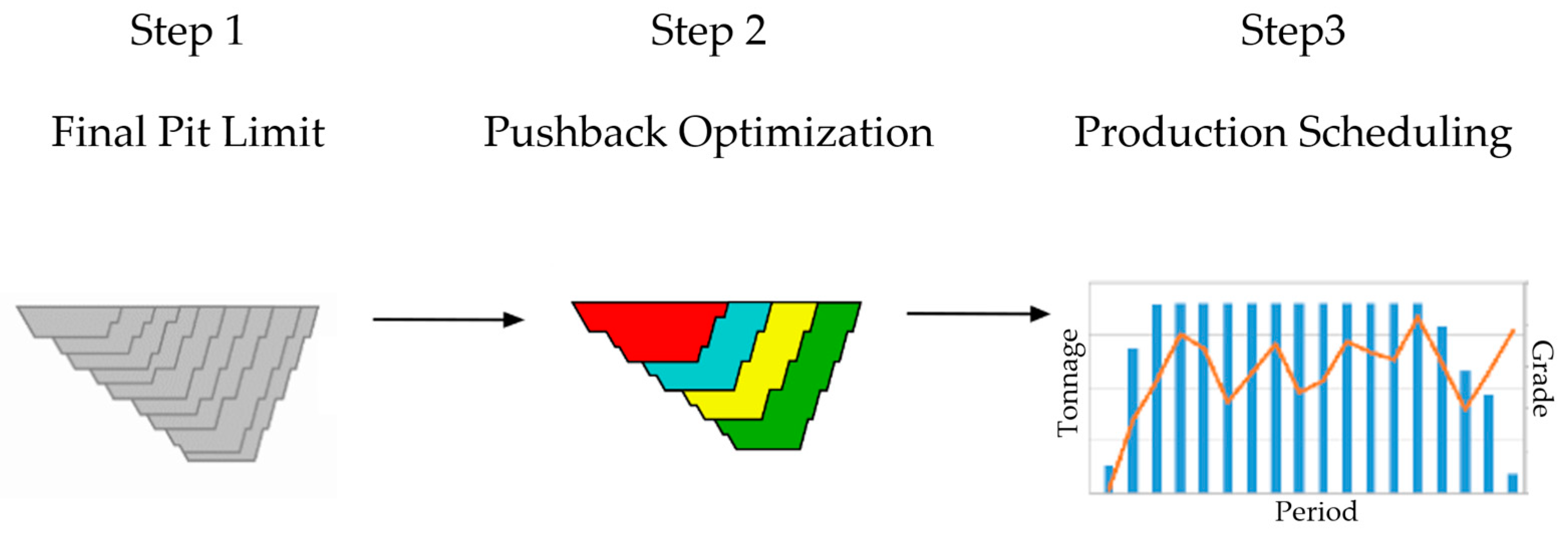
• Economic evaluation. For each block, an economic evaluation representing the net economic value of mining it (and potentially processing it) is calculated. This evaluation depends on the block’s mineral content, the price of the ore, and the associated costs of mining and processing the block. Thus, an economic block model is obtained.
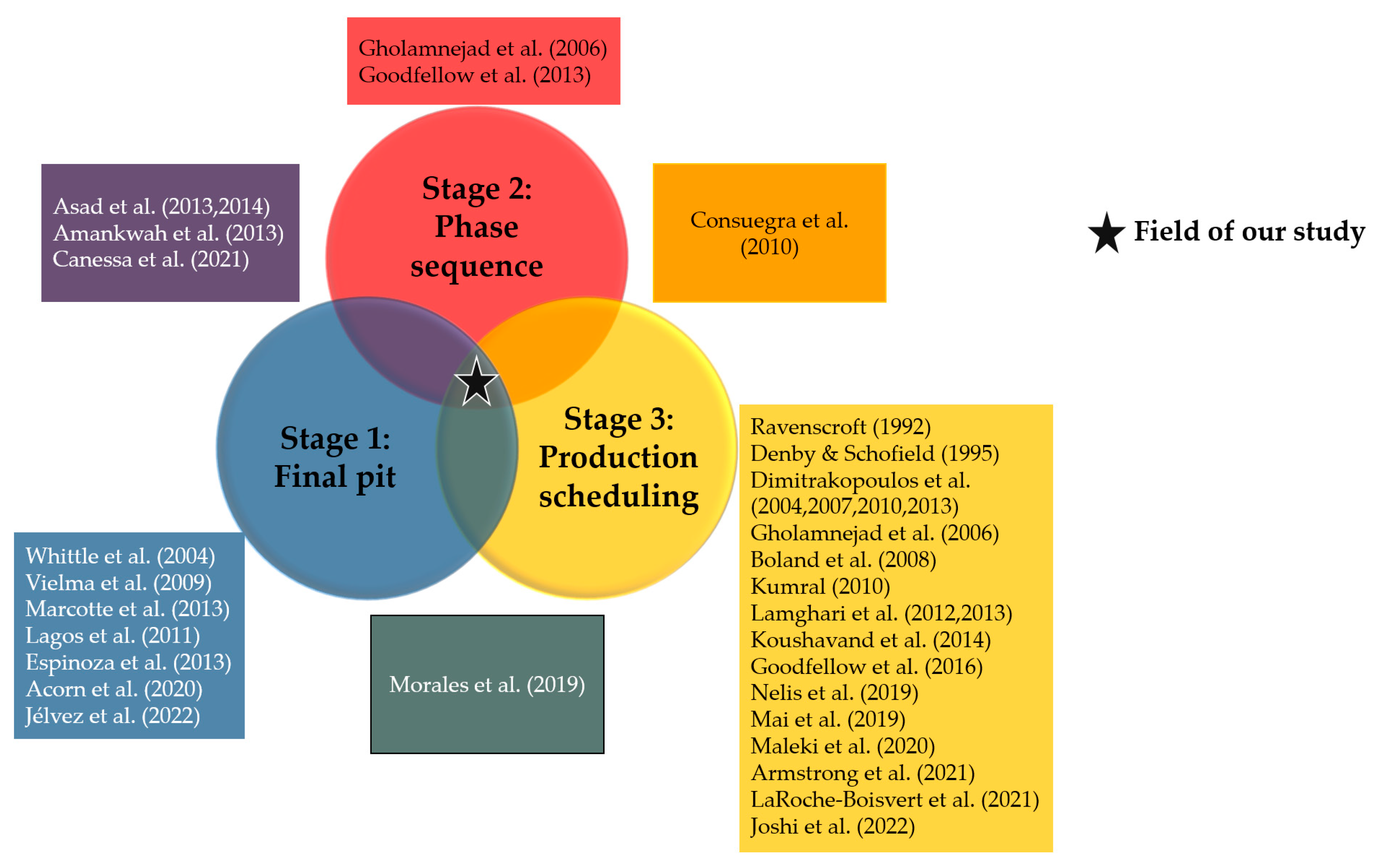
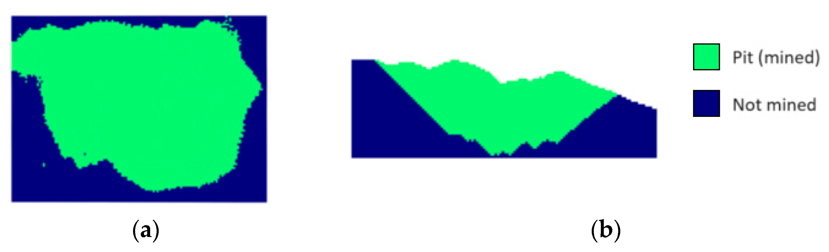
• Final pit. With this main input, in addition to a series of technical parameters, the region of the mine where the exploitation will be carried out is defined; this is known as the final pit (first stage). This key step in the planning process provides an estimation of the economic value and tonnage of the mining project in its early stages.
• Pushback optimization. Within the final pit, many incremental nested pits are generated using the Lerchs and Grossmann methodology [4]. Among these nested pits, some are chosen to define the mining phases (second stage), and the volumes between consecutive phases are called pushbacks. The selection of the phases (equivalently, the pushbacks) is performed based on selected criteria, such as the minimum operational width that must be maintained to ensure an operative design and similar ore tonnage [5,6,7,8].
• Production scheduling. Within each phase, the ore production is scheduled over time (third stage), committing during the life of the mine to the quantity and quality of material to be extracted and processed, generating the promise of value that maximizes the NPV of the mining business [9,10,11].

Figure 1 shows a schematic diagram of the traditional production planning process of an open pit mine, from the final pit computation to the production scheduling.

The above stages seek to ensure an open pit mine that maximizes the net present value but, at the same time, is operationally feasible. However, a critical drawback of the standard planning workflow is the assumption of perfect knowledge. For example, the process assumes a known and stable performance of the mining equipment for each time period. However, the complexity of mining operations and the uncertainty associated with shovels and trucks—which is usually known as operational uncertainty—can impact the fulfillment of production forecasts in the long term [13]. Moreover, fluctuations in prices or costs—known as market uncertainty—can also be detrimental to the fulfillment of the expected net present value of the mining project [14].

In this work, we focus on geological uncertainty, which represents the degree of ignorance in the mineralogical characterization of the geological resource and relates mainly to the uncertainty associated with the estimation of grades.

Ignoring uncertainty can have consequences on different scales. In the final pit definition, where uncertainty is higher, it increases the risk of economic losses and strongly constrains the next stages; in the definition of phases, it prevents identifying risky sectors within the final pit, which can present deviations in the final production scheduling stage.

In the traditional methodology, all three stages are solved using some strategic mine planning software. According to [9], most commercial software packages use the nested pits method or similar implementations. Consequently, they may result in production plans that are difficult to fulfill in practice because they do not consider geological uncertainty [15,16].

Because of the above, many research studies have shown that the incorporation of geostatistical simulations, each representing a probable grade distribution of the same deposit, has shown better results in the assessment of the value of the business since they reproduce the real spatial variability of the variables. In particular, the use of conditional simulations [17,18,19] has allowed the inclusion of this type of uncertainty into the production planning process.

Some efforts have been made to develop approaches that incorporate geological uncertainty. In the final pit definition stage, early works have assessed the impact of uncertainty in calculating final pits for several scenarios [20] and based on the expected value of each block [21]. Risk-averse and robust approaches have also been studied [22,23,24] alongside efficient-frontier analysis for a defined set of risk levels [25,26]. However, most of the research in this area omits the subsequent stages to assess the impact of the final pit definition under uncertainty.

Pushback optimization is important in the traditional mine planning workflow since it integrates operational constraints, such as a minimum mining width, into the mine schedule. However, the inclusion of uncertainty at this stage has been mostly omitted in the literature. Early works evaluated the impact of including grade uncertainty at this stage [27]. Reducing the economic value of blocks with high-grade variability has been proposed to obtain nested pits with high value and low risk [28]. Selecting nested pits based on minimizing deviations from production targets has also been implemented [29]. These approaches have not been integrated into the production scheduling stage to evaluate the impact of the pushback definition.

Production scheduling under uncertainty has been the most widely studied stage in the planning workflow for open-pit mines. Early works quantified the potential of including uncertainty in production scheduling [30,31,32], and several approaches have been proposed. One of the most widely used approaches is the minimization of deviation from production targets, which generates schedules that maximize NPV and minimize penalties for not fulfilling tonnage, grade, or quality goals [33,34,35,36,37,38,39]. Two-stage stochastic programs have also been implemented to include recourse actions when new information arrives [40,41,42]. Robust optimization has also been used to make resilient stochastic schedules under grade uncertainty [43]. Most stochastic production scheduling models pose a significant computational challenge. For this reason, a wide range of algorithms, heuristics, and metaheuristics have been implemented to offer reasonable computation times for this problem [44,45,46,47,48,49]. In this stage, most works use a deterministic final pit as a base and then implement a stochastic production scheduling model within the pit limits, i.e., they omit the pushback optimization. As a result, the obtained stochastic solutions are difficult to implement in the operation, and the economic values of the solutions are not realistic.

A few efforts have been made to integrate some of the three stages of strategic planning. For instance, a stochastic network-flow algorithm was proposed to include uncertainty in the traditional parametrization of the nested pit problem [50,51] to integrate stages 1 and 2. Risk-averse models using the conditional value-at-risk have also been studied to define the final pit and the phase design [52,53]. In terms of the integration of the final pit limit and production scheduling, the reliability of the final pit under grade uncertainty, and the minimization of deviations in the mine schedule were evaluated [12]. Finally, the effect of selecting nested pits and generating a stochastic schedule under geological uncertainty was also explored in [54].

A complete review of models and algorithms that have been performed in the last two decades to address the integration of uncertainty in mine planning can be found at [55,56,57,58]. Figure 2 shows a diagram of the major research that has been done to address each of the different stages of the production planning process under geological uncertainty. As shown in the figure, our field of study lies at the intersection of all stages. To the best of our knowledge, there are no studies that evaluate the inclusion of uncertainty in all three stages.

This paper proposes a multi-stage methodology to define the final pit, pushback optimization, and production scheduling. We use models based on mixed integer linear programming that incorporate geological uncertainty in each of the stages to maximize the expected NPV and, at the same time, minimize the risk of losses associated with this source of uncertainty. Specifically, this paper contributes:

• A mathematical model to optimize the final pit considering the geological uncertainty. The model optimizes the pit value minus the conditional value at risk (CVaR).
• A mathematical model for pushback optimization in an uncertainty setting. In the application in this paper, the model selects pushbacks from nested pits such that the total tonnages are similar, but it can be modified to accommodate other criteria.
• A mixed-integer program to schedule bench phases under uncertainty to minimize deviations from production targets based on an existing set of pushbacks.
• The integration of the previous contributions as a multi-stage strategic optimization approach and its application in a real case study.

Besides the novelty of the models and the methodology, it is worth noting that our work is the first to address the three stages simultaneously, which allowed us to analyze the effect of uncertainty at the different stages, which can be used to help engineers focus their efforts for modeling over the different stages of the planning process. Finally, it is worth mentioning that even though we present our approach in the context of geological uncertainty, the models could also be used for market uncertainty.

2. Materials and Methods

This section introduces the mathematical notation and optimization models we propose for each planning stage. For the final pit definition, we propose a model that maximizes expected NPV and minimizes a risk metric. For the pushback optimization, we extend a methodology that selects nested pits to form pushbacks presented in [6], but with the integration of a stochastic NPV for each block inside the final pit from stage 1. Finally, for the production scheduling, we propose a novel optimization model that maximizes expected NPV and minimizes deviations from production targets using the pushbacks from stage 2.

2.1. General Notation

First, $\mathit{B}$ represents the block model. The blocks are denoted with the letter $b$, identified by their centroid $(x,y,z)\in {\mathbb{R}}^3$. Multiple realizations (conditional simulations) of the mineral resource model are considered to incorporate the geological uncertainty, and they are indexed by $\mathit{S}=\{1,\dots ,S\}$. If the random variable representing the element concentration of block $b$ is ${\mathit{g}}_b$, then ${\left\{g_{bs}\right\}}_{s\in \mathit{S}}$ represents a set of realizations or samples of $g_b$.

Due to stability requirements, slope constraints are given by one or several slope angles that define the maximum slopes that are possible in the pit walls. The standard way to model these slope constraints is to use arcs of precedence as follows: For any given block $b$, there exists a set $\mathit{P}\mathit{R}\mathit{E}{\mathit{C}}_b\subset \mathit{B}-\left\{b\right\}$ of other blocks (called predecessors) that must be mined before to gain access to block b and keep the pit walls stable. Figure 3 shows a simple configuration based on a 45° slope angle and one level of precedence. In the figure, to extract block 6, the first five blocks (1, 2, 3, 4, and 5) must be removed. In this case, $PRE{C}_6=\{1, 2, 3, 4, 5\}$ (left). On the other hand, the 2D view shows in blue arrows the arcs of precedence induced for a given slope angle (right).

To generate the economic block model, we consider the simplest case for extracted blocks: (i) They are classified as ore blocks (revenues > costs) and therefore can be sent for processing, or (ii) they are classified as waste blocks, in which case these blocks are sent to waste dumps. Under scenario $s\in \mathit{S}$, the economic value of a block that is mined and processed is given by:

$$va{l}_{bs}^{proc}=to{n}_b\left(price\cdot rec\cdot g_{bs}-mcost-pcost\right) \left(\mathrm{USD}\right)$$

(1)

If a block is treated as waste, its economic value is given by:

$$va{l}_b^{dump}=-mcost\cdot to{n}_b (\mathrm{USD})$$

(2)

The net economic value of a block is therefore calculated as:

$$v_{bs}=\max \left\{va{l}_{bs}^{proc}, va{l}_b^{dump}\right\} (\mathrm{USD})$$

(3)

In the previous equations, $price$ is the metal price [USD/ton], $rec$ is the average metallurgical recovery (in percent), $g_{bs}$ is the concentration of the metal of interest (grade, as a fraction) in block $b$ when geological scenario $s$ is considered, $mcost$ and $pcost$ are mining and processing costs [USD/ton], and $to{n}_b$ is the tonnage of block $b$.

Note that the grade $g_{bs}$ of block $b$ and scenario $s$ is replaced by ${\overline{g}}_b$ for the deterministic case, i.e., when no uncertainty is considered. In this case, the net value of a block $b$ is expressed as ${\overline{v}}_b$.

2.2. Stage 1: Final Pit Limit Problem

In this section, we propose an optimization model that maximizes the expected net undiscounted value and simultaneously minimizes the risk of losses, expressed in terms of the value at risk (VaR) and the conditional value at risk (CVaR) [59]. We use a discrete approximation of VaR and CVaR [60], noted $\widetilde{VaR}$ and $\widetilde{CVaR}$, respectively, which allows using a sample from the probability distribution of $g$, given by scenarios generated by conditional simulation.

The decision variables are defined as

$$x_b=\left\{\begin{array}{l}1, \mathrm{i}\mathrm{f} \mathrm{b}\mathrm{l}\mathrm{o}\mathrm{c}\mathrm{k} b \mathrm{b}\mathrm{e}\mathrm{l}\mathrm{o}\mathrm{n}\mathrm{g}\mathrm{s} \mathrm{t}\mathrm{o} \mathrm{t}\mathrm{h}\mathrm{e} \mathrm{f}\mathrm{i}\mathrm{n}\mathrm{a}\mathrm{l} \mathrm{p}\mathrm{i}\mathrm{t} \mathrm{l}\mathrm{i}\mathrm{m}\mathrm{i}\mathrm{t},\\ 0, \mathrm{o}\mathrm{t}\mathrm{h}\mathrm{e}\mathrm{r}\mathrm{w}\mathrm{i}\mathrm{s}\mathrm{e}\end{array}\right.$$

(4)

$$z_s=Contribution of scenario s to \widetilde{CVaR}$$

(5)

We propose the following mixed integer linear programming model that maximizes the difference between the expected total value and $\widetilde{CVaR}$:

$\left(\mathrm{P}1\right)$	$\mathit{max} \frac{1}{S}\left({\displaystyle \sum _{b\in \mathit{B},s\in \mathit{S}}}{v}_{bs}\cdot x_b\right)-\widetilde{CVaR}$		(6)
s.t.	$x_b\le x_{b^{\prime }}$	$\forall b\in \mathit{B},b^{\prime }\in \mathit{P}\mathit{R}\mathit{E}{\mathit{C}}_{\mathit{b}}$	(7)
	${\mathrm{z}}_{\mathrm{s}}\ge f\left(x,g^s\right)-\widetilde{VaR}$	$\forall s\in \mathit{S}$	(8)
	$f\left(x,g^s\right)={\displaystyle \sum _{b\in \mathit{B}}}\left({\overline{v}}_b-v_{bs}\right)x_b$	$\forall s\in \mathit{S}$	(9)
	$\widetilde{CVaR}=\widetilde{VaR}+\frac{1}{S(1-\delta )}{\displaystyle \sum _{s\in \mathit{S}}}{z}_s$	$\forall s\in \mathit{S}$	(10)
	$z_s\ge 0$	$\forall s\in \mathit{S}$	(11)
	$x_b\in \left\{\mathrm{0,1}\right\}$	$\forall b\in \mathit{B}$	(12)

Equation (6) represents the objective function. Equation (7) corresponds to the precedence constraints given by the slope angle. Equations (8)–(10) establish the conditions for a well-defined discrete CVaR (in this context, loss function $f$ represents the monetary loss obtained in scenario $s$ w.r.t. the base/deterministic case), with $\delta \in \left(\mathrm{0,1}\right)$ the confidence level, and Equations (11) and (12) state the nature of variables, continuous and binary, respectively.

An optimal solution of $\left(P1\right)$ determines which blocks belong to the final pit limit so that the expected value is maximized throughout all simulations while minimizing the risk of losses measured by the discrete approximation of CVaR. The deterministic version of this problem can be found in [61].

2.3. Stage 2: Pushback Optimization

In the above subsection, a stochastic final pit was determined. Now, a procedure for pushback optimization (stage 2) is presented. The procedure accounts for the geological uncertainty within the final pit and extends the ideas presented in [6], where the deterministic case is studied. This extension considers multiple realizations of the orebody and consists of two parts: computation of stochastic nested pits and pushback selection. We describe them now.

2.3.1. Computation of Stochastic Nested Pits

Let ${\mathit{B}}^{\prime }\subseteq \mathit{B}$ be the ultimate pit limit obtained from Section 2.1. Applying the methodology of Lerchs and Grossmann [4] and scaling the metal price by a series of $n$ revenue factors $0<{\lambda }_1<\cdots <{\lambda }_n$, we have a value $v_{bs}^i$ for each block $b$, each realization $s$ and each revenue factor ${\lambda }_k$ given by:

$$va{l}_{bs}^{proc}=to{n}_b({\lambda }_k\cdot price\cdot rec\cdot g_{bs}-mcost-pcost) (\mathrm{USD})$$

(13)

Averaging block values over all realizations, we have an expected value of each block $b$ associated with the revenue factor ${\lambda }_i$ given by:

$$v_b^i=S^{-1}{\sum }_{s\in \mathit{S}}{v}_{bs }^i (\mathrm{USD})$$

(14)

To obtain the stochastic nested pits, we solve $n$ final pit limit problems, one for each ${\lambda }_k$, according to [21], obtaining $\varnothing ={\mathit{P}}_0\subseteq {\mathit{P}}_1\subseteq \cdots \subseteq {\mathit{P}}_n$ nested pits, where ${\mathit{P}}_n={\mathit{B}}^{\prime }$.

2.3.2. Pushback Selection from the Stochastic Nested Pits

From the potentially many pits generated in the previous stage, we are going to select some of them as mining phases. The pushbacks correspond to the volume between consecutively selected pits; thus, selecting pits or pushbacks is equivalent.

To select pushbacks from the set of stochastic nested pits, we use the formulation proposed in [6], where an optimization model chooses the best pushback candidates based on minimizing the gap problem [5] so that the resulting phases have the minimum difference among them in ore and waste tonnages. For this, we define a pushback $\mathit{P}\mathit{u}\mathit{s}{\mathit{h}}_{jk}={\mathit{P}}_j\setminus {\mathit{P}}_k$ as the set of blocks contained between nested pits ${\mathit{P}}_j$ and ${\mathit{P}}_k$, where $1\le k<j\le n.$ Given pushback $\mathit{P}\mathit{u}\mathit{s}{\mathit{h}}_{jk}$ we extend block attributes such as ore tonnage ($oto{n}_{jk})$ or rock tonnage$\left(rto{n}_{jk}\right)$ by adding individual values. To partition ${\mathit{B}}^{\prime }$ into pushbacks, it is necessary to define the set of preceding pushbacks (Equation (15)) and the set of succeeding pushbacks (Equation (16)) of$Pus{h}_{jk}$.

$$\mathit{P}\mathit{R}\mathit{E}{\mathit{C}}_{jk}=\left\{\mathit{P}\mathit{u}\mathit{s}{\mathit{h}}_{j{k}^{\prime }}:k^{\prime }\in \overline{0,k-1}\right\} \forall j\in \overline{2,n},k\in \overline{1,j-1}$$

(15)

$$\mathit{S}\mathit{U}{\mathit{C}}_{jk}=\left\{\mathit{P}\mathit{u}\mathit{s}{\mathit{h}}_{j^{\prime }k}:j^{\prime }\in \overline{j+1,n}\right\} \forall j\in \overline{1,n-1},k\in \overline{0,j-1}$$

(16)

From the above, the decision variables are defined as

$$x_{jk}=\left\{\begin{array}{cc}1& \mathrm{if}Pus{h}_{jk}\mathrm{is}\mathrm{chosen} \mathrm{as} \mathrm{a} \mathrm{mining} \mathrm{phase}\\ 0& \mathrm{otherwise}\end{array}\right.$$

(17)

In our model, we will assume that we are interested in minimizing differences between phase tonnages (other goals/constraints can be considered similarly). For this, we use the mean absolute deviation (MAD), where the tonnages are compared to a reference value$rto{n}_{N0}/n_o$, when $n_o$ phases are desired. Then, the integer linear programming model that minimizes MAD is

$\left(\mathrm{P}2\right)$	$\mathit{min} \frac{1}{n_o}{\displaystyle \sum _{\begin{array}{c}j\in \overline{1,n} \\ k\in \overline{0,j-1}\end{array}}}\left|rto{n}_{jk}-\frac{rto{n}_{n0}}{n_o}\right|\cdot x_{jk}$		(18)
s.t.	${\displaystyle \sum _{\begin{array}{c}j\in \overline{1,n} \\ k\in \overline{0,j-1}\end{array}}}{x}_{jk}=n_o$		(19)
	${\displaystyle \sum _{\begin{array}{c}j\in \overline{1,n} \end{array}}}{x}_{j0}=1$		(20)
	${\displaystyle \sum _{\begin{array}{c}k\in \overline{0,n-1}\end{array}}}{x}_{nk}=1$		(21)
	$x_{jk}\le {\displaystyle \sum _{\begin{array}{c}\mathit{P}\mathit{u}\mathit{s}{\mathit{h}}_{j^{\prime }{k}^{\prime }}\in \mathit{P}\mathit{R}\mathit{E}{\mathit{C}}_{jk}\end{array}}}{x}_{j^{\prime }{k}^{\prime }}$	$\forall j\in \overline{2,n},k\in \overline{1,j-1}$	(22)
	$x_{jk}\le {\displaystyle \sum _{\begin{array}{c}\mathit{P}\mathit{u}\mathit{s}{\mathit{h}}_{j^{\prime }{k}^{\prime }}\in \mathit{S}\mathit{U}{\mathit{C}}_{jk}\end{array}}}{x}_{j^{\prime }{k}^{\prime }}$	$\forall j\in \overline{1,n-1},k\in \overline{0,j-1}$	(23)
	${\displaystyle \sum _{\begin{array}{c}\mathit{P}\mathit{u}\mathit{s}{\mathit{h}}_{j^{\prime }{k}^{\prime }}\in \mathit{P}\mathit{R}\mathit{E}{\mathit{C}}_{jk}\end{array}}}{x}_{j^{\prime }{k}^{\prime }}\le 1$	$\forall j\in \overline{2,n},k\in \overline{1,j-1}$	(24)
	${\displaystyle \sum _{\begin{array}{c}\mathit{P}\mathit{u}\mathit{s}{\mathit{h}}_{j^{\prime }{k}^{\prime }}\in \mathit{S}\mathit{U}{\mathit{C}}_{jk}\end{array}}}{x}_{j^{\prime }{k}^{\prime }}\le 1$	$\forall j\in \overline{1,n-1},k\in \overline{0,j-1}$	(25)
	$x_{jk}\in \left\{\mathrm{0,1}\right\}$	$\forall j\in \overline{1,n},k\in \overline{0,j-1}$	(26)

Equation (18) represents the objective function. Equation (19) sets the number of desired phases. Equations (20)–(25) determine the partitioning of the final pit into phases, specifically: Equations (20) and (21) impose the selection of an initial pit ${\mathit{P}}_0$ and an ultimate pit$P_n$, respectively; Equations (22) and (24) enforce that to select a pushback, one and only one preceding pushback must be selected. Similarly, Equations (23) and (25) establish that to select a given pushback, one and only one succeeding pushback is selected. Finally, Equation (26) states the binary nature of variables.

2.4. Stage 3: Production Scheduling

Once the final pit limit and the pushbacks have been defined, mine production must be scheduled over time (third stage). In this section, we develop the methodology for generating a production schedule based on the set of pushbacks defined in the previous stage.

In the last few years, some authors have presented different models that aim to maximize NPV and minimize the negative effects of uncertainty [12,36,39,44,62,63,64]. A common approach to these models is based on the incorporation of penalties that reduce the expected NPV when production or quality targets are not met. These penalties are usually defined by the magnitude of the deviation from the required target and a deviation cost.

In this case, we consider that due to geological uncertainty, production schedules may suffer deviations in practice, generating issues of under-production or over-production, whether from ore to process or ore quality (blending) that is not in the range of acceptance. The following notation is considered: the unitary costs per ore (metal) tonnage of over- and under-production at period $t$ on scenario $s$ are represented as $c{p}_{ts}^{+}$ and $c{p}_{ts}^{-}$ ($c{g}_{ts}^{+}$ and ${cg}_{ts}^{-})$, respectively.

Since the deposit was partitioned into a set of $n_0$ pushbacks, to have control over the extraction geometry and organize the equipment, the $p$th pushback is denoted as ${\mathit{B}}_p$, with ${\mathit{B}}^{\prime }={\bigcup }_{p=1}^{n_0}{\mathit{B}}_p.$ Furthermore, benches are defined as the set of all blocks having the same z-coordinate. The intersection of a phase and a bench is called a bench phase or panel, which will be denoted by

$${\mathit{B}}_p^j=\left\{\left(x,y,z\right)\in {\mathit{B}}_p:z=z\left(j\right)\right\}\hspace{1em}\forall j\in \overline{1,J_p}$$

(27)

where $J_p$ represents the number of benches inside phase $p$. We assume the relation $z\left(1\right)>z\left(2\right)>\cdots >z\left(J_p\right)$, so that we can identify each bench phase using an index $j$.

We consider a time horizon $T\in \mathbb{N}$ and denote individual time periods with $t=\mathrm{1,2},...,T$. The set of time periods is denoted by $\mathit{T}=\overline{1,T}$. There is also a set of destinations $\mathit{D}=\mathit{P}\cup \mathit{W}$ composed of a set of processing plants $\mathit{P}$ and a set of waste dumps $\mathit{W}$. For example, $d\in \mathit{P}$ can be considered as a processing plant in Equation (1), or $d\in \mathit{W}$ the waste dump in Equation (2). The discounted value for a block $b\in \mathit{B}$ in geological scenario $s\in \mathit{S}$ when sent to destination $d\in \mathit{D}$ in period $t\in \mathit{T}$ is given by

$$v_{bdts}={\rho }^t{v}_{bds} \left(\mathrm{USD}\right)$$

(28)

where $\rho$ is a discount rate representing the opportunity cost. The stochastic value ${\overline{v}}_{bdt}$is obtained by averaging over all geological scenarios.

For each block, we identify two sets of attributes: (i) Those related to the quantity of material and control of the available operational resource, such as ore and waste tonnages; and (ii) those related to the concentration of a given element, such as ore grades or pollutants. In particular, we define $rto{n}_b$ as the total tonnage (ore + waste) of block$b$. To account for grade uncertainty, $g_{bs}$ and $oto{n}_{bs}$ are defined as the ore grade and ore tonnage, respectively, of each block $b$ in scenario$s$. These definitions will be useful to control deviations from the production targets. The upper and lower limits are denoted, respectively, by (i) mining capacity in period $t$, $M{C}_t^{+}$ and $M{C}_t^{-}$; (ii) processing capacity for $d\in \mathit{P}$ in period $t$, $P{C}_{dt}^{+}$ and $P{C}_{dt}^{-}$; and (iii) blending or quality of ore grade for $d\in \mathit{P}$ in period $t$, $B{C}_{dt}^{+}$ and $B{C}_{dt}^{-}$.

The formulation considers the extraction and processing decisions separately, using binary variables for the first one and continuous variables for the second one, making it a mixed integer program. The objective function is the usual maximization of NPV while simultaneously minimizing the total discounted cost associated with deviations from production targets.

The decision variable is defined for$b\in {\mathit{B}}^{\prime }$, $t\in \mathit{T}$:

$$x_{bt}=\left\{\begin{array}{c}1, \mathrm{i}\mathrm{f} \mathrm{b}\mathrm{l}\mathrm{o}\mathrm{c}\mathrm{k} b \mathrm{i}\mathrm{s} \mathrm{e}\mathrm{x}\mathrm{t}\mathrm{r}\mathrm{a}\mathrm{c}\mathrm{t}\mathrm{e}\mathrm{d} \mathrm{b}\mathrm{y} \mathrm{p}\mathrm{e}\mathrm{r}\mathrm{i}\mathrm{o}\mathrm{d} t, \\ 0, \mathrm{o}\mathrm{t}\mathrm{h}\mathrm{e}\mathrm{r}\mathrm{w}\mathrm{i}\mathrm{s}\mathrm{e} \end{array}\right.$$

(29)

The interpretation of variable $x_{bt}$ is by period, that is $x_{bt}=1$ if and only if block $b$ has been extracted at some period $s\in \overline{1,t}$. The advantages of this formulation are discussed in [65]. To simplify the notation, it is useful to introduce the following auxiliary variables for $b\in B$: ${\mathsf{\Delta }x}_{b1}=x_{b1}$, and $\mathsf{\Delta }{x}_{bt}=x_{bt}-x_{b,t-1}$ for $t=\overline{2,T}$. We have $x_{bt}=\sum _{s\le t}{x}_{bs}$ and $\mathsf{\Delta }{x}_{bt}=1$ if, and only if, the block $b$ is extracted exactly at period $t$.

The second set of variables are defined for $b\in \mathit{B}$, $d\in \mathit{D}$, and $t\in \mathit{T}$:

$$y_{bdt}=\mathrm{fraction} \mathrm{of} \mathrm{block} b \mathrm{sent} \mathrm{to} \mathrm{destination} d \mathrm{at} \mathrm{period} t$$

(30)

A third set of binary variables controls the progress of bench-phases in the operation, defined for phase $p\in \overline{1,n_o}$, bench $j\in \overline{1,J_p}$, and period $t\in \mathit{T}$:

$$z_{pjt}=\left\{\begin{array}{cc}1,& \begin{array}{c}\mathrm{i}\mathrm{f} \mathrm{b}\mathrm{e}\mathrm{n}\mathrm{c}\mathrm{h}\text{-}\mathrm{p}\mathrm{h}\mathrm{a}\mathrm{s}\mathrm{e} {\mathit{B}}_p^j \mathrm{i}\mathrm{s} \mathrm{c}\mathrm{o}\mathrm{m}\mathrm{p}\mathrm{l}\mathrm{e}\mathrm{t}\mathrm{e}\mathrm{l}\mathrm{y} \mathrm{e}\mathrm{x}\mathrm{t}\mathrm{r}\mathrm{a}\mathrm{c}\mathrm{t}\mathrm{e}\mathrm{d} \mathrm{b}\mathrm{y} \mathrm{p}\mathrm{e}\mathrm{r}\mathrm{i}\mathrm{o}\mathrm{d} t\end{array}\\ 0,& \mathrm{otherwise}.\end{array}\right.$$

(31)

Finally, we define continuous variables to represent the deviations from the ore production target and average metal requirement. For each, we define both under and over deviations, for $t\in \mathit{T}$ and $s\in \mathit{S}$ in Equations (32)–(35).

$$u_{ts}^{-}=\mathrm{d}\mathrm{e}\mathrm{f}\mathrm{i}\mathrm{c}\mathrm{i}\mathrm{t} \mathrm{o}\mathrm{f} \mathrm{e}\mathrm{x}\mathrm{t}\mathrm{r}\mathrm{a}\mathrm{c}\mathrm{t}\mathrm{e}\mathrm{d} \mathrm{o}\mathrm{r}\mathrm{e} \mathrm{t}\mathrm{o}\mathrm{n}\mathrm{s} \mathrm{a}\mathrm{t} \mathrm{p}\mathrm{e}\mathrm{r}\mathrm{i}\mathrm{o}\mathrm{d} t \mathrm{a}\mathrm{n}\mathrm{d} \mathrm{s}\mathrm{c}\mathrm{e}\mathrm{n}\mathrm{a}\mathrm{r}\mathrm{i}\mathrm{o} s.$$

(32)

$$u_{ts}^{+}=\mathrm{s}\mathrm{u}\mathrm{p}\mathrm{e}\mathrm{r}\mathrm{a}\mathrm{v}\mathrm{i}\mathrm{t} \mathrm{o}\mathrm{f} \mathrm{e}\mathrm{x}\mathrm{t}\mathrm{r}\mathrm{a}\mathrm{c}\mathrm{t}\mathrm{e}\mathrm{d} \mathrm{o}\mathrm{r}\mathrm{e} \mathrm{t}\mathrm{o}\mathrm{n}\mathrm{s} \mathrm{a}\mathrm{t} \mathrm{p}\mathrm{e}\mathrm{r}\mathrm{i}\mathrm{o}\mathrm{d} t \mathrm{a}\mathrm{n}\mathrm{d} \mathrm{s}\mathrm{c}\mathrm{e}\mathrm{n}\mathrm{a}\mathrm{r}\mathrm{i}\mathrm{o} s.$$

(33)

$$v_{ts}^{-}=\mathrm{d}\mathrm{e}\mathrm{f}\mathrm{i}\mathrm{c}\mathrm{i}\mathrm{t} \mathrm{o}\mathrm{f} \mathrm{m}\mathrm{e}\mathrm{t}\mathrm{a}\mathrm{l} \mathrm{p}\mathrm{r}\mathrm{o}\mathrm{d}\mathrm{u}\mathrm{c}\mathrm{t}\mathrm{i}\mathrm{o}\mathrm{n} \mathrm{t}\mathrm{o}\mathrm{n}\mathrm{s} \mathrm{a}\mathrm{t} \mathrm{p}\mathrm{e}\mathrm{r}\mathrm{i}\mathrm{o}\mathrm{d} t \mathrm{a}\mathrm{n}\mathrm{d} \mathrm{s}\mathrm{c}\mathrm{e}\mathrm{n}\mathrm{a}\mathrm{r}\mathrm{i}\mathrm{o} s.$$

(34)

$${ v}_{ts}^{+}=\mathrm{s}\mathrm{u}\mathrm{p}\mathrm{e}\mathrm{r}\mathrm{a}\mathrm{v}\mathrm{i}\mathrm{t} \mathrm{o}\mathrm{f} \mathrm{m}\mathrm{e}\mathrm{t}\mathrm{a}\mathrm{l} \mathrm{p}\mathrm{r}\mathrm{o}\mathrm{d}\mathrm{u}\mathrm{c}\mathrm{t}\mathrm{i}\mathrm{o}\mathrm{n} \mathrm{t}\mathrm{o}\mathrm{n}\mathrm{s} \mathrm{a}\mathrm{t} \mathrm{p}\mathrm{e}\mathrm{r}\mathrm{i}\mathrm{o}\mathrm{d} t \mathrm{a}\mathrm{n}\mathrm{d} \mathrm{s}\mathrm{c}\mathrm{e}\mathrm{n}\mathrm{a}\mathrm{r}\mathrm{i}\mathrm{o} s.$$

(35)

Then, the mixed integer linear programming model to generate a production schedule, following a balanced order of phases, and not allowing a depth greater than a certain threshold $\Phi \in \mathbb{N}$ between consecutive phases, is given by Equations (36)–(52).

(P3)	$max\frac{1}{S}\left({\displaystyle \sum _{\begin{array}{c}b\in \mathit{B}, t\in \mathit{T}\\ d\in \mathit{D}, s\in \mathit{S}\end{array}}}{v}_{bdts}\cdot y_{bdt}-{\displaystyle \sum _{t\in \mathit{T},s\in \mathit{S}}}c{p}_{ts}^{+}{u}_{ts}^{+}+c{p}_{ts}^{-}{u}_{ts}^{-}+c{g}_{ts}^{+}{v}_{ts}^{+}+c{g}_{ts}^{-}{v}_{ts}^{-}\right)$		(36)
s. t.	$\mathsf{\Delta }{x}_{bt}\ge 0$	$\forall b\in {\mathit{B}}^{\prime },t\in \mathit{T}$	(37)
	$\mathsf{\Delta }{x}_{bt}={\displaystyle \sum _{d\in \mathit{D}}}{y}_{bdt}$	$\forall b\in {\mathit{B}}^{\prime },t\in \mathit{T}$	(38)
	$z_{p\left(j-1\right)t}\le x_{bt}$	$\forall b\in {\mathit{B}}_p^{j-1},t\in \mathit{T},p\in \overline{1,n_o},j\in \overline{2,J_p}$	(39)
	$x_{bt}\le z_{p\left(j-1\right)t}$	$\forall b\in {\mathit{B}}_p^j,t\in \mathit{T},p\in \overline{1,n_o},j\in \overline{2,J_p}$	(40)
	$x_{bt}\le z_{p\left(j-\Phi \right)t}$	$\forall b\in {\mathit{B}}_{p-1}^j,t\in \mathit{T},p\in \overline{2,n_o},j\in \overline{\Phi +1,J_{p-1}}$	(41)
	$x_{bt}\le z_{(p-1)jt}$	$\forall b\in {\mathit{B}}_p^{j-\Phi +1},t\in \mathit{T},p\in \overline{2,n_o},j\in \overline{\Phi ,J_{p-1}}$	(42)
	${\displaystyle \sum _{b\in \mathit{B}}}rto{n}_b\cdot \mathsf{\Delta }{x}_{bt}\le M{C}_t^{+}$	$\forall t\in \mathit{T}$	(43)
	${\displaystyle \sum _{b\in \mathit{B}}}rto{n}_b\cdot \mathsf{\Delta }{x}_{bt}\ge M{C}_t^{-}$	$\forall t\in \mathit{T}$	(44)
	${\displaystyle \sum _{b\in \mathit{B}}}oto{n}_{bs}\cdot y_{bdt}-u_{ts}^{+}\le P{C}_{dt}^{+}$	$\forall t\in \mathit{T},s\in \mathit{S},d\in \mathit{P}$	(45)
	${\displaystyle \sum _{b\in \mathit{B}}}oto{n}_{bs}\cdot y_{bdt}+u_{ts}^{-}\ge P{C}_{dt}^{-}$	$\forall t\in \mathit{T},s\in \mathit{S},d\in \mathit{P}$	(46)
	${\displaystyle \sum _{b\in \mathit{B}}}\left(g_{bs}-B{C}_{dt}^{+}\right)\cdot oto{n}_{bs}\cdot y_{bdt}\le v_{ts}^{+}$	$\forall s\in \mathit{S},t\in \mathit{T},d\in \mathit{P}$	(47)
	${\displaystyle \sum _{b\in B}}\left(B{C}_{dt}^{-}-g_{bs}\right)\cdot oto{n}_{bs}\cdot y_{bdt}\le v_{ts}^{-}$	$\forall s\in \mathit{S},t\in \mathit{T},d\in \mathit{P}$	(48)
	$x_{bt}\in \left\{\mathrm{0,1}\right\}$	$\forall b\in {\mathit{B}}^{\prime },t\in \mathit{T}$	(49)
	$z_{pjt}\in \left\{\mathrm{0,1}\right\}$	$\forall p\in \overline{1,n_o},j\in \overline{1,J_p},t\in \mathit{T}$	(50)
	$y_{bdt}\in \left[\mathrm{0,1}\right]$	$\forall b\in {\mathit{B}}^{\prime },d\in \mathit{D},t\in \mathit{T}$	(51)
	$u_{ts}^{+},u_{ts}^{-},v_{ts}^{+},v_{ts}^{-}\ge 0$	$\forall t\in \mathit{T},s\in \mathit{S}$	(52)

Equation (36) presents the objective function, which is the maximum expected NPV of the mine schedule minus the cost of uncertainty, i.e., the total cost associated with deviations from the production targets. Equation (37) restricts each block to being extracted only once, and Equation (38) requires the values of the extraction and processing variables to be consistent, i.e., if a block is extracted, then it must be distributed among the possible destinations. In turn, Equations (39) and (40) correspond to the vertical precedence constraints between mining benches, and Equations (41) and (42) impose an order in the balanced sequence of extraction between benches from different phases. In addition, Equations (43) and (44) limit the consumption of mining (hauling) resources in each period, which affects ore and waste material. In turn, Equations (45) and (46) limit the consumption of processing resources in each period $t$and scenario$s$, which constrains the amount of ore treated at the plant. Similarly, Equations (47) and (48) represent the blending constraints over the average ore grade at destination $d$ for each scenario $s$ and period$t$. Finally, Equation (49) establishes that extraction variables are binary. Equation (50) represents the binary variables that control the precedence between consecutive benches. Equation (51) indicates that the processing variables are continuous, and Equation (52) represents the deviations in the production objectives.

2.5. Case Study

The block model is a porphyry copper deposit from northern Chile, for which 50 conditional simulations are available. This model consists of 407,179 blocks of 10 m × 10 m × 10 m. The average grade among 50 scenarios is used as a deterministic representation of the copper grade variable. For confidentiality reasons, other specific aspects of the block model, such as owner and location, among others, are not disclosed.

Figure 4a presents the histogram, including error bars along simulations, and Figure 4b shows grade–tonnage curves to quantify the recoverable resources at different cut-off grades. Both figures represent error bars with the 5th and 95th percentiles per interval, showing low uncertainty in copper grades and ore tonnages.

The parameters to generate economic block values are presented in

Table 1. Economic and technical parameters to evaluate the 2D model.

Parameter	Symbol	Value
Copper price (USD/ton)	Price	5511.55
Metallurgical recovery	Rec	0.85
Mining cost (USD/ton)	Mcost	3.2
Processing cost (USD/ton)	Pcost	9.0

. The methodology is applied by considering the following parameters. For the final pit limit, a confidence level of $\delta =95\%$. For the pushback optimization, the revenue factors are ${\lambda }_k=\frac{k}{90},$ with $k\in \overline{\mathrm{1,90}}$. The parameters for production scheduling are presented in

Table 2. Economic and technical parameters for production scheduling.

Parameter	Symbol	Value
Max. mining capacity (Mton)	$M{C}_t^{+}$	13.0
Min. mining capacity (Mton)	$M{C}_t^{-}$	0.0
Max. processing capacity (Mton)	$P{C}_t^{+}$	7.0
Min. processing capacity (Mton)	$P{C}_t^{-}$	6.0
Max. average grade (%)	$B{C}_{dt}^{+}$	$+\infty$
Min. average grade (%)	$B{C}_{dt}^{-}$	0.8–0.5
Maximum depth (benches)	$\mathsf{\Phi }$	8
Horizon planning (years)	$T$	22
Discount rate	$\rho$	1/(1 + 10%)
Number of destinations	$D$	2
Number of scenarios	$S$	50
Cost over-production ore (USD/ton)	$c{p}_{s0}^{+}$	18.5
Cost under-production ore (USD/ton)	$c{p}_{s0}^{-}$	18.5
Cost over-production metal (USD/ton)	$c{g}_{s0}^{+}$	0
Cost under-production metal (USD/ton)	$c{g}_{s0}^{-}$	39.0

.

3. Results

This section presents and analyzes the results obtained corresponding to each stage of the proposed methodology for the case study. Optimization models were coded in Python (PuLP library, version 2.5.1) [66] with GUROBI 8.1.1 [67] and executed on a 64-bit Windows OS (version 10 Pro) workstation with a CPU Intel Xeon E5 2660 v3 with 128 Gb RAM.

3.1. Final Pit

Table 3. Numerical results for a final pit limit by considering CVaR as a risk measure with a confidence level $\delta =95\%$.

VaR [MUSD]	CVaR [MUSD]	Exptd. Value [MUSD]	Opt. Gap (%)	Time [s]
144.99	166.00	2078.06	0.1	14,881

shows a summary of the numerical results: Risk measures VaR and CVaR, expected undiscounted value, optimality gap, and CPU processing time, by considering a confidence level of 95%. The results show an expected undiscounted value equal to $2078.06 \mathrm{M}\mathrm{U}\mathrm{S}\mathrm{D}$, with a 95% probability, the loss does not exceed $VaR=144.99 \mathrm{M}\mathrm{U}\mathrm{S}\mathrm{D}$ and the average of the 5% highest losses will not exceed $CVaR=166.00 \mathrm{M}\mathrm{U}\mathrm{S}\mathrm{D}$. The expected ore tonnage is 137.52 [Mton] and the expected rock tonnage is 273.19 [Mton]. The shape of the resulting final pit is presented in Figure 5. The stochastic final pit limit problem was solved in about 4 h.

3.2. Pushback Optimization

Ninety nested pits ${\mathit{P}}_1\subseteq {\mathit{P}}_2\subseteq \cdots \subseteq {\mathit{P}}_{90}$ were generated (Figure 6): The first non-empty pit is $\lambda =\frac{17}{90}$; therefore, the first 16 pits are empty. Figure 7 shows the “pit by pit” graph, including error bars (P95-P5 band) for both ore tonnage as well as expected economic values for each pit.

Note that both the expected tonnage of waste and ore are strictly increasing, but the first one has a higher growth rate than the second one, which in general indicates that the pushbacks will present an increasing stripping ratio (the amount of waste material that must be removed to release a given ore quantity). In fact, the first pit will present a low stripping ratio, an ideal scenario to ensure a production scheduling that maximizes the cumulative discounted expected value, subject to operational constraints.

Model $\left(P_2\right)$ is then used to select 4 pushbacks to reduce the differences in ore and waste tonnages among the resulting phases. The model has $(n-3)(n-2)(n-1)/6=\mathrm{113,564}$ ways to perform the partition of the final pit. Figure 8 shows the 4 phases (plan and section views), and Figure 9 shows the tonnages of ore and waste and average grade per phase, including the associated error bars (P5 and P95) according to the grade variability. We highlight that there are decreasing ore tonnage and average grades along the phases. The total CPU time was 300 [s] for the computation of stochastic nested pits and 15 [s] for solving the phase selection model$\left(P_2\right)$.

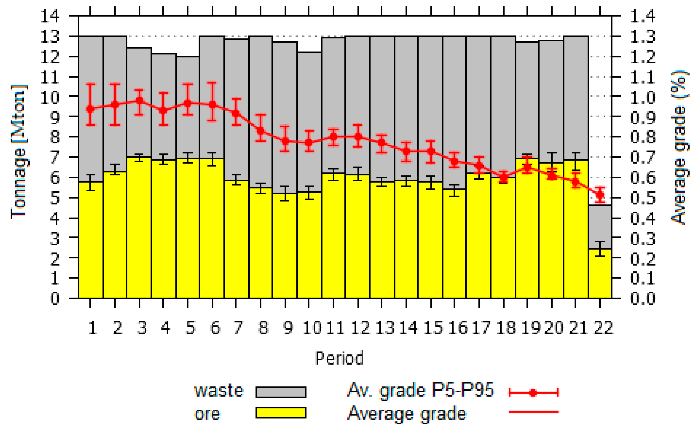
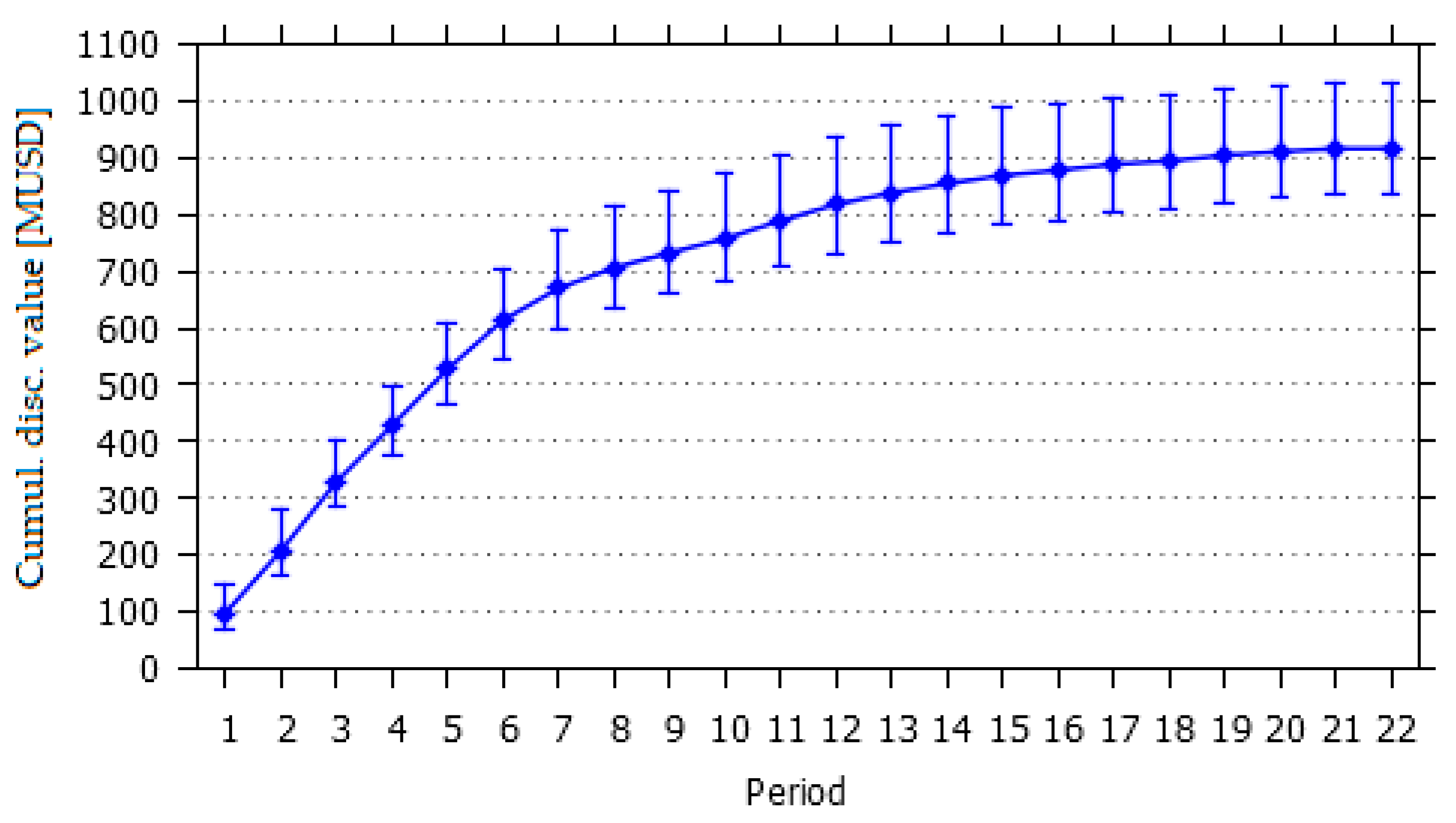
3.3. Production Scheduling

Different constraints were applied to limit the upper and lower mining capacities as well as the processing capacities. In addition, we ensure sufficient quality ore for mill feed by imposing a lower limit on the average grade per period, which is decreasing, as seen in Stage 2: we applied a lower limit of 0.8% for the first 7 periods and 0.7%, 0.6%, and 0.5% for each of the following 3 five-year periods, respectively.

Figure 10 shows the bench phases scheduled: The extraction fulfills the maximum lead constraint of eight benches between contiguous phases. This requirement is common in traditional long-term planning workflows and ensures that the resulting schedule is operationally feasible. Ignoring this requirement could lead to potentially higher NPV solutions that are difficult to implement in the operation. This constraint was imposed over all phases, but it is possible to restrict this choice to a smaller number of phases and to change the depth, all according to the evaluator’s requirements. Figure 11 shows the production plan, including ore and waste tonnages per period, along with the average grade of mill feed.

In this stage, the production scheduling model assigns the destination of each block based on its value, production capacities, and deviations from targets. Depending on the ore distribution in the deposit, the model can impose a different cut-off grade for each period. This is usually noted as a dynamic cut-off grade policy. In contrast, in stage 1, the block destination is an input for the final pit problem and is based solely on the block’s value. This is usually denoted as a fixed cut-off grade policy. To compare the effects of both strategies,

Table 4. A comparison of expected ore, waste, and rock tonnages by considering fixed and dynamic cutoff grades.

Expected Tonnage [Mton]	Cutoff Grade		Difference [Ton]	Relative Variation %
	Fixed	Dynamic
Ore	137.52	131.72	5.80	4.4
Waste	135.67	141.47	−5.80	−4.1
Total (rock)	273.19	273.19	0.00	0.0

shows the expected tonnages for each policy: There are 5.8 [Mton] of rejected ore, as in the final pit, 137.5 [Mton] of ore were reported, but in the scheduling, only 131.7 [Mton] were sent to the processing plant. The rock tonnages matched, showing that the final pit was fully scheduled. Figure 12 shows the cumulative discounted expected value of the project, reaching a total of 916.5 [MUSD], with a P95-P5 range of 197 [MUSD].

3.4. Impact of Grade Uncertainty at Each of the Planning Stages

In this section, we present the effect of incorporating grade uncertainty at different stages of the proposed methodology. For this purpose, four cases are evaluated, depending on whether a stochastic approach ($S$) or deterministic approach ($D$) is considered:

• Fully deterministic, “$(D, D, D)$”: In this case, the multi-stage methodology is applied without considering grade uncertainty, i.e., under a deterministic approach. This is considered the “base case”.
• Stochastic 3rd stage, “$(D, D, S)$”: This case aims to evaluate the effect of incorporating grade uncertainty in production scheduling only. For this, we consider grade uncertainty only in stage 3, deterministic final pit, and pushback optimization.
• Deterministic 1st stage, “$(D, S, S)$”: In this case, the final pit limit is chosen under a deterministic approach, but pushback optimization and production scheduling are stochastic.
• Fully stochastic, “$(S, S, S)$”: In this case, the multi-stage methodology is applied, considering grade uncertainty at all stages. This case aims to evaluate the contribution of Stage 1 under grade uncertainty when compared with$(D,S,S)$. Additionally, this case shows the added value of the complete proposed methodology.

Table 5. Results of multi-stage methodology incorporating grade uncertainty in different stages.

Case	ENPV [MUSD]	Relative Variation of ENPV (%)	ETCU [MUSD]	Relative Variation of ETCU (%)
$(D,D,D)$	904.7	-	86.5	-
$(D,D,S)$	915.4	0.9	41.8	−51.7
$(D,S,S)$	917.8	1.1	34.2	−60.5
$(S,S,S)$	923.8	2.1	26.7	−69.1

presents, for each case, the expected net present value (ENPV), the expected total cost of uncertainty (ETCU), and their relative variations (in percentage) with respect to the base case. In this case study, the ENPV may increase by up to 2.1%, and the ETCU associated with deviations from production targets can be reduced by up to 69%, which illustrates how the proposed methodology can control the risk of economic losses.

We observe that the total value of information is $ENP{V}_{S,S,S}-ENP{V}_{D,D,D}=19.1$ [MUSD], where stage 1 (final pit limit) contributes 31.4%, stage 2 (pushback optimization) contributes 12.6%, and stage 3 (production scheduling) contributes 56%. This is very interesting because it means that the impact of the selection of the final pit is very significant (almost 1/3) and that more than half of the value is related to scheduling. It is also interesting to note that pushback optimization does not play a significant role. However, these conclusions depend on the case study and the proposed methodology; thus, they can be different in other deposits or if the models used to address each of the stages are different.

On a more general note, this shows how the multi-stage sequential approach could be applied to determine the relative impact of different stages and, therefore, where to invest the most effort to improve the value and reduce the potential cost of uncertainty.

4. Conclusions

This paper addressed the problem of the long-term open-pit mine production planning process under grade uncertainty, using a multi-stage sequential approach that generalizes the current practice of computing a final pit, then selecting mining phases, and, finally, scheduling production over time. The objective was to investigate the negative effects of geological uncertainty at different stages of the planning process. Robust models that incorporate this representation of uncertainty in mine planning were proposed and assessed. Results show that incorporating uncertainty helps reduce the risk of losses due to failure to meet production goals as compared with the fully deterministic case. However, the uncertainty does not affect all stages equally, so it is particularly interesting to deepen these experiments through more case studies and new models and algorithms that incorporate geological uncertainty at different stages.

In future work, we propose to consider rock type uncertainty in addition to grade uncertainty. It is necessary to research new algorithms to find near-optimal solutions quickly, especially in stages 1 and 3. Finally, we propose to incorporate more practical mining constraints, such as minimum mining widths, into the proposed models (stages 2 and 3).

References

1. Hustrulid, W.A.; Kuchta, M.; Martin, R.K. Open Pit Mine Planning and Design, Two Volume Set & CD-ROM Pack; CRC Press: Boca Raton, FL, USA, 2013. [Google Scholar] [CrossRef]
2. Chilès, J.-P.; Delfiner, P. Geostatistics Modeling Spatial Uncertainty; John Wiley & Sons: New York, NY, USA, 2012; Available online: http://internationalscholarvoxcom/book/88813008 (accessed on 24 June 2018).
3. Tabesh, M.; Mieth, C.; Nasab, H.A. A multi-step approach to long-term open-pit production planning. Int. J. Min. Miner. Eng. 2014, 5, 273. [Google Scholar] [CrossRef]
4. Lerchs, H.; Grossmann, I.F. Optimum Design of Open-Pit Mines, Transactions. Can. Inst. Min. 1965, 58, 17–24. [Google Scholar]
5. Meagher, C.; Dimitrakopoulos, R.; Avis, D. Optimized open pit mine design, pushbacks and the gap problem—A review. J. Min. Sci. 2014, 50, 508–526. [Google Scholar] [CrossRef]
6. Jélvez, E.; Morales, N.; Askari-Nasab, H. A new model for automated pushback selection. Comput. Oper. Res. 2020, 115, 104456. [Google Scholar] [CrossRef]
7. Nancel-Penard, P.; Morales, N. Optimizing pushback design considering minimum mining width for open pit strategic planning. Eng. Optim. 2022, 54, 1494–1508. [Google Scholar] [CrossRef]
8. Morales, N.; Nancel-Penard, P.; Espejo, N. Development and analysis of a methodology to generate operational open-pit mine ramp designs automatically. Optim. Eng. 2022, 24, 711–741. [Google Scholar] [CrossRef]
9. Chicoisne, R.; Espinoza, D.; Goycoolea, M.; Moreno, E.; Rubio, E. A New Algorithm for the Open-Pit Mine Production Scheduling Problem. Oper. Res. 2012, 60, 517–528. [Google Scholar] [CrossRef]
10. Letelier, O.R.; Espinoza, D.; Goycoolea, M.; Moreno, E.; Muñoz, G. Production Scheduling for Strategic Open Pit Mine Planning: A Mixed-Integer Programming Approach. Oper. Res. 2020, 68, 1425–1444. [Google Scholar] [CrossRef]
11. Nancel-Penard, P.; Morales, N.; Cornillier, F. A recursive time aggregation-disaggregation heuristic for the multidimensional and multiperiod precedence-constrained knapsack problem: An application to the open-pit mine block sequencing problem. Eur. J. Oper. Res. 2022, 303, 1088–1099. [Google Scholar] [CrossRef]
12. Morales, N.; Seguel, S.; Cáceres, A.; Jélvez, E.; Alarcón, M. Incorporation of Geometallurgical Attributes and Geological Uncertainty into Long-Term Open-Pit Mine Planning. Minerals 2019, 9, 108. [Google Scholar] [CrossRef]
13. Upadhyay, S.; Askari-Nasab, H. Simulation and optimization approach for uncertainty-based short-term planning in open pit mines. Int. J. Min. Sci. Technol. 2018, 8, 153–166. [Google Scholar] [CrossRef]
14. Abdel Sabour, S.A.; Dimitrakopoulos, R.G.; Kumral, M. Mine design selection under uncertainty. Min. Technol. 2008, 117, 53–64. [Google Scholar] [CrossRef]
15. Dowd, P.A.; Xu, C.; Coward, S. Strategic mine planning and design: Some challenges and strategies for addressing them. Min. Technol. 2016, 125, 22–34. [Google Scholar] [CrossRef]
16. Dimitrakopoulos, R. Advances in Applied Strategic Mine Planning; Springer: Cham, Switzerland, 2018. [Google Scholar]
17. Ortiz, J.M.; Deutsch, C.V. Indicator Simulation Accounting for Multiple-Point Statistics. Math. Geol. 2004, 36, 545–565. [Google Scholar] [CrossRef]
18. Emery, X.; Lantuéjoul, C. TBSIM: A computer program for conditional simulation of three-dimensional Gaussian random fields via the turning bands method. Comput. Geosci. 2006, 32, 1615–1628. [Google Scholar] [CrossRef]
19. Maleki, M.; Madani, N.; Jélvez, E. Geostatistical Algorithm Selection for Mineral Resources Assessment and its Impact on Open-pit Production Planning Considering Metal Grade Boundary Effect. Nat. Resour. Res. 2021, 30, 4079–4094. [Google Scholar] [CrossRef]
20. Whittle, D. A Bozorgebrahimi, Hybrid Pits—Linking Conditional Simulation and Lerchs-Grossmann Through Set Theory. In Proceedings of the Symposium on Orebody Modelling and Strategic Mine Planning, Perth, Australia, 22–24 November 2004; pp. 399–404. [Google Scholar]
21. Marcotte, D.; Caron, J. Ultimate open pit stochastic optimization. Comput. Geosci. 2013, 51, 238–246. [Google Scholar] [CrossRef]
22. Vielma, J.P.; Espinoza, D.; Moreno, E. Risk control in ultimate pits using conditional simulations. In Proceedings of the 34th APCOM Conference, Vancouver, BC, Canada, 6–9 October 2009; pp. 107–114. [Google Scholar]
23. Lagos, G.; Espinoza, D.; Moreno, E.; Amaya, J. Robust Planning for an Open-Pit Mining Problem under Ore-Grade Uncertainty. Electron. Notes Discret. Math. 2011, 37, 15–20. [Google Scholar] [CrossRef]
24. Espinoza, D.; Lagos, G.; Moreno, E.; Vielma, J. Risk averse approaches in open-pit production planning under ore grade uncertainty: An ultimate pit study. In Proceedings of the 36th International Symposium on the Applications of Computers and Operations Research in the Mineral Industry (APCOM), Alegre, Brazil, 4–8 November 2013; pp. 492–501. [Google Scholar]
25. Acorn, T.; Boisvert, J.B.; Leuangthong, O. Managing Geologic Uncertainty in Pit Shell Optimization Using a Heuristic Algorithm and Stochastic Dominance, Mining. Metall. Explor. 2020, 37, 375–386. [Google Scholar] [CrossRef]
26. Jelvez, E.; Morales, N.; Ortiz, J.M. Stochastic Final Pit Limits: An Efficient Frontier Analysis under Geological Uncertainty in the Open-Pit Mining Industry. Mathematics 2021, 10, 100. [Google Scholar] [CrossRef]
27. Dimitrakopoulos, R.; Martinez, L.; Ramazan, S. A maximum upside/minimum downside approach to the traditional optimization of open pit mine design. J. Min. Sci. 2007, 43, 73–82. [Google Scholar] [CrossRef]
28. Gholamnejad, J.; Osanloo, M. Incorporation of ore grade uncertainty into the push back design process. J. South. Afr. Inst. Min. Metall. 2007, 107, 177–185. [Google Scholar]
29. Goodfellow, R.; Dimitrakopoulos, R. Algorithmic integration of geological uncertainty in pushback designs for complex multiprocess open pit mines. Min. Technol. 2013, 122, 67–77. [Google Scholar] [CrossRef]
30. Ravenscroft, P. Risk analysis for mine scheduling by conditional simulation. Trans. Inst. Min. Metall. Sect. A Min. Ind. 1992, 101, A104–A108. [Google Scholar]
31. Denby, B.; Schofield, D. Inclusion of risk assessment in open-pit design and scheduling. Int. J. Rock. Mech. Min. Sci. Geomech. Abstr. 1995, 5, 230A. [Google Scholar]
32. Dimitrakopoulos, R.; Farrelly, C.T.; Godoy, M. Moving forward from traditional optimization: Grade uncertainty and risk effects in open-pit design. Min. Technol. 2002, 111, 82–88. [Google Scholar] [CrossRef]
33. Dimitrakopoulos, R.; Ramazan, S. Uncertainty based production scheduling in open pit mining. SME Trans. 2004, 316, 106–112. [Google Scholar]
34. Dimitrakopoulos, R. Stochastic optimization for strategic mine planning: A decade of developments. J. Min. Sci. 2011, 47, 138–150. [Google Scholar] [CrossRef]
35. Dimitrakopoulos, R.; Jewbali, A. Joint stochastic optimisation of short and long term mine production planning: Method and application in a large operating gold mine. Min. Technol. 2013, 122, 110–123. [Google Scholar] [CrossRef]
36. Koushavand, B.; Askari-Nasab, H.; Deutsch, C.V. A linear programming model for long-term mine planning in the presence of grade uncertainty and a stockpile. Int. J. Min. Sci. Technol. 2014, 24, 451–459. [Google Scholar] [CrossRef]
37. Mai, N.L.; Topal, E.; Erten, O.; Sommerville, B. A new risk-based optimisation method for the iron ore production scheduling using stochastic integer programming. Resour. Policy 2019, 62, 571–579. [Google Scholar] [CrossRef]
38. Maleki, M.; Jélvez, E.; Emery, X.; Morales, N. Stochastic Open-Pit Mine Production Scheduling: A Case Study of an Iron Deposit. Minerals 2020, 10, 585. [Google Scholar] [CrossRef]
39. LaRoche-Boisvert, M.; Dimitrakopoulos, R. An Application of Simultaneous Stochastic Optimization at a Large Open-Pit Gold Mining Complex under Supply Uncertainty. Minerals 2021, 11, 172. [Google Scholar] [CrossRef]
40. Boland, N.; Dumitrescu, I.; Froyland, G. A multistage stochastic programming approach to open pit mine production scheduling with uncertain geology. Optim. Online 2008, 1–33. [Google Scholar]
41. Nelis, G.; Morales, N.; Widzyk-Capehart, E. Comparison of Different Approaches to Strategic Open-Pit Mine Planning Under Geological Uncertainty. In Proceedings of the 27th International Symposium on Mine Planning and Equipment Selection-MPES 2018, Calgary, AL, Canada, 4–22 August 2018; Widzyk-Capehart, E., Hekmat, A., Singhal, R., Eds.; Springer International Publishing: Cham, Switzerland, 2019; pp. 95–105. [Google Scholar] [CrossRef]
42. Armstrong, M.; Lagos, T.; Emery, X.; Homem-de-Mello, T.; Lagos, G.; Sauré, D. Adaptive open-pit mining planning under geological uncertainty. Resour. Policy 2021, 72, 102086. [Google Scholar] [CrossRef]
43. Kumral, M. Robust stochastic mine production scheduling. Eng. Optim. 2010, 42, 567–579. [Google Scholar] [CrossRef]
44. Lamghari, A.; Dimitrakopoulos, R. Progressive hedging applied as a metaheuristic to schedule production in open-pit mines accounting for reserve uncertainty. Eur. J. Oper. Res. 2016, 253, 843–855. [Google Scholar] [CrossRef]
45. Goodfellow, R.C.; Dimitrakopoulos, R. Global optimization of open pit mining complexes with uncertainty. Appl. Soft Comput. 2016, 40, 292–304. [Google Scholar] [CrossRef]
46. Chatterjee, S.; Dimitrakopoulos, R. Production scheduling under uncertainty of an open-pit mine using Lagrangian relaxation and branch-and-cut algorithm. Int. J. Min. Reclam. Environ. 2020, 34, 343–361. [Google Scholar] [CrossRef]
47. Lamghari, A.; Dimitrakopoulos, R. Hyper-heuristic approaches for strategic mine planning under uncertainty. Comput. Oper. Res. 2020, 115, 104590. [Google Scholar] [CrossRef]
48. Tolouei, K.; Moosavi, E.; Tabrizi, A.H.; Afzal, P.; Bazzazi, A.A. An optimisation approach for uncertainty-based long-term production scheduling in open-pit mines using meta-heuristic algorithms. Int. J. Min. Reclam. Environ. 2021, 35, 115–140. [Google Scholar] [CrossRef]
49. Joshi, D.; Paithankar, A.; Chatterjee, S.; Equeenuddin, S.M. Integrated Parametric Graph Closure and Branch-and-Cut Algorithm for Open Pit Mine Scheduling under Uncertainty. Mining 2022, 2, 32–51. [Google Scholar] [CrossRef]
50. Asad, M.W.; Dimitrakopoulos, R. Implementing a parametric maximum flow algorithm for optimal open pit mine design under uncertain supply and demand. J. Oper. Res. Soc. 2013, 64, 185–197. [Google Scholar] [CrossRef]
51. Asad, M.W.; Dimitrakopoulos, R.; van Eldert, J. Stochastic production phase design for an open pit mining complex with multiple processing streams. Eng. Optim. 2014, 46, 1139–1152. [Google Scholar] [CrossRef]
52. Amankwah, H.; Larsson, T.; Textorius, B. Open-Pit Mining with Uncertainty: A Conditional Value-at-Risk Approach. In Optimization Theory, Decision Making, and Operations Research Applications; Migdalas, A., Sifaleras, A., Georgiadis, C.K., Papathanasiou, J., Stiakakis, E., Eds.; Springer: New York, NY, USA, 2013; pp. 117–139. [Google Scholar] [CrossRef]
53. Canessa, G.; Moreno, E.; Pagnoncelli, B.K. The risk-averse ultimate pit problem. Optim. Eng. 2021, 22, 2655–2678. [Google Scholar] [CrossRef]
54. Consuegra, F.R.; Dimitrakopoulos, R. Algorithmic approach to pushback design based on stochastic programming: Method, application and comparisons. Min. Technol. 2010, 119, 88–101. [Google Scholar] [CrossRef]
55. Osanloo, M.; Gholamnejad, J.; Karimi, B. Long-term open pit mine production planning: A review of models and algorithms, International Journal of Mining. Reclam. Environ. 2008, 22, 3–35. [Google Scholar] [CrossRef]
56. Fathollahzadeh, K.; Asad, M.W.; Mardaneh, E.; Cigla, M. Review of Solution Methodologies for Open Pit Mine Production Scheduling Problem. Int. J. Min. Reclam. Environ. 2021, 35, 564–599. [Google Scholar] [CrossRef]
57. Zeng, L.; Liu, S.Q.; Kozan, E.; Corry, P.; Masoud, M. A comprehensive interdisciplinary review of mine supply chain management. Resour. Policy 2021, 74, 102274. [Google Scholar] [CrossRef]
58. Dimitrakopoulos, R.; Lamghari, A. Simultaneous stochastic optimization of mining complexes-mineral value chains: An overview of concepts, examples and comparisons. Int. J. Min. Reclam. Environ. 2022, 36, 443–460. [Google Scholar] [CrossRef]
59. Rockafellar, R.T.; Uryasev, S. Optimization of conditional value-at-risk. JOR 2000, 2, 21–41. [Google Scholar] [CrossRef]
60. Krokhmal, P.; Uryasev, S.; Palmquist, J. Portfolio optimization with conditional value-at-risk objective and constraints. JOR 2001, 4, 43–68. [Google Scholar] [CrossRef]
61. Espinoza, D.; Goycoolea, M.; Moreno, E. A Newman, MineLib: A library of open pit mining problems. Ann. Oper. Res. 2013, 206, 93–114. [Google Scholar] [CrossRef]
62. Dimitrakopoulos, R.; Ramazan, S. Stochastic integer programming for optimising long term production schedules of open pit mines: Methods, application and value of stochastic solutions. Min. Technol. 2008, 117, 155–160. [Google Scholar] [CrossRef]
63. Leite, A.; Dimitrakopoulos, R. Stochastic optimization of mine production scheduling with uncertain ore/metal/waste supply. Int. J. Min. Sci. Technol. 2014, 24, 755–762. [Google Scholar] [CrossRef]
64. de Carvalho, J.; Dimitrakopoulos, R. Effects of High-Order Simulations on the Simultaneous Stochastic Optimization of Mining Complexes. Minerals 2019, 9, 210. [Google Scholar] [CrossRef]
65. Lambert, W.B.; Brickey, A.; Newman, A.M.; Eurek, K. Open-Pit Block-Sequencing Formulations: A Tutorial. Interfaces 2014, 44, 127–142. [Google Scholar] [CrossRef]
66. Mitchell, S.; OSullivan, M.; Dunning, I. PuLP: A Linear Programming Toolkit for Python; The University of Auckland: Auckland, New Zealand, 2011. [Google Scholar]
67. Gurobi Optimization, LCC. Gurobi Optimizer Reference Manual 2022. 2022. Available online: http://www.gurobi.com (accessed on 30 June 2022).
Figure 1. Traditional methodology for long-term open-pit mine planning [12].
Mathematics 11 03907 g001
Figure 2. Related work in different stages of open-pit mine production planning process under geological uncertainty and field of our study.
Mathematics 11 03907 g002
Figure 3. Precedence relationship between blocks for a given slope angle for a given block “6”. Left: Isometric view of immediate predecessors 1–5. Right: Section view with some predecessors ans slope angle.
Mathematics 11 03907 g003
Figure 4. Summary of the 3D block model: (a) Histogram of copper grades, including error bars (P5 and P95 percentiles), (b) grade–tonnage curves for the set of simulated realizations (P5 and P95) and deterministic geological model.
Mathematics 11 03907 g004
Figure 5. Stochastic final pit limit by considering a confidence level δ = 95 % . (a) Plan view, (b) north section view—5.030 m.
Mathematics 11 03907 g005
Figure 6. (a) Stochastic nested pits inside final pit limit from stage 1: (a) Plan view, (b) N section view—5.030 m.
Mathematics 11 03907 g006
Figure 7. “Pit by pit” graph, considering both ore tonnage and undiscounted value variability due to geological uncertainty.
Mathematics 11 03907 g007
Figure 8. (a) Stochastic pushback optimization inside the final pit limit from stage 1: (a) Plan view, (b) N section view—5.030 m.
Mathematics 11 03907 g008
Figure 9. Ore and waste tonnages (primary Y axis), and average grade (secondary Y axis) per pushback, including error bars (P5 and P95) due to grade variability.
Mathematics 11 03907 g009
Figure 10. Scheduled blocks respecting the pushback optimization. (a) Plan view, (b) N section view—5.030 m.
Mathematics 11 03907 g010
Figure 11. Production plan: ore and waste tonnages, including error bars (P5 and P95) in ore (left Y axis), and average grade of mill feed (secondary Y axis).
Mathematics 11 03907 g011
Figure 12. Cumulative discounted expected value from the production schedule. P95–P5 range is included to show the variability along geological realizations.
Mathematics 11 03907 g012