Analysis of a Pre-Emptive Two-Priority Queuing System with Impatient Customers and Heterogeneous Servers

Abstract

This paper presents a queuing system model that incorporates multiple priorities, multiple abandonments, and heterogeneous servers. Waiting for service easily leads to impatient behaviors. The impact of two kinds of impatient behaviors, balking and reneging, on queueing system performance is examined. The problem is formulated as continuous-time Markov chains. It also introduces a special state called the non-sojourn state to record the number of customers who abandon the system. The state transition rate matrix is transformed into a block tridiagonal matrix by appropriately setting the state numbers. A novel indicator called interstate transition frequency is proposed, which aids in distinguishing state transitions during the system evaluation process. Based on the interstate transition frequency, a set of indicators is derived to offer additional analytical perspectives for the queuing system. Finally, the proposed model is applied to an automobile repair shop to validate its effectiveness in practical scenarios.

1. Introduction

The increasing integration and intelligentization of industrial modernization have led to a gradual rise in the proportion of equipment maintenance and labor costs within the total cost. Therefore, controlling this cost has become a new focal point in the field of equipment maintenance and management. Queuing theory and Markov processes have laid a solid foundation for operating cost analysis and have attracted widespread attention. However, in practice, traditional models are difficult to widely use in actual production processes due to their lack of flexibility. Therefore, conducting research on a new queuing model that considers priority, abandonment, and heterogeneous servers is of practical significance.

The existing research on priority and abandonment in queuing systems can be summarized as follows. Jaiswal [1] introduced the concept of priority scheduling with the resumption of service of a low-priority customer. Kleinrock [2] proposed a time-dependent priority queue and derived the expressions for the average waiting times for different priorities. Priorities can be classified into two categories [3]: pre-emptive priority [4,5,6], in which a higher-priority customer entering the system will cause any ongoing work to be interrupted, and the maintainer will immediately serve the higher-priority customer, and non-pre-emptive priority [7], in which a customer with priority entering the system will be placed at the front of the queue automatically.

The concept of abandonment was initially proposed by Halfin [8]. Aguir [9] categorized impatient actions into three situations: balking, reneging, and retrial. In terms of balking rules, Height [10] and Garnett [11] determined whether malfunctioning equipment entered the system with queue length and system load. If the number of waiting customers or the workload falls below a threshold, the customer will enter the system; otherwise, they will leave. In the case of reneging, there is an upper boundary of waiting time generated when a customer enters the system. If the waiting time exceeds the threshold, the customer will leave due to a lack of patience. Wei [12] defined the waiting time as a constant, Wang [13] considered individual differences and modeled the waiting time as an exponential distribution, and Ward [14] extended the distribution of the waiting time to accommodate arbitrary distributions. Comprehensive reviews of retrials were provided by Falin [15] and Artalejo [16], wherein customers have the option to re-enter the system and join the queue after leaving.

Most studies on queuing systems traditionally separate the prioritization and abandonment mechanisms. However, as queuing theory advanced, the integration of these two aspects has become increasingly prevalent. For instance, research has emerged on service differentiation problems in multiclass queuing systems that consider class-dependent services and abandonment distributions. Takagi [17] derived explicit expressions using Laplace-Stieltjes transforms for an M/M/m pre-emptive-loss last-come-first-serve (LCFS) system with impatient customers, as well as an M/M/m pre-emptive-resume LCFS queue with patient customers. Additionally, Jouini [18] examined scenarios involving multiple servers and non-pre-emptive customers.

The quantity and types of personnel are critical factors in research. Brandwajn [19] proposed a mathematical approach to compute the steady-state queue length distribution in first-come-first-serve (FCFS) queues with homogeneous server numbers. Bouchentouf [20] conducted an analysis of a heterogeneous two-server queuing system. Liu [21] investigated a service differentiation problem in a multiclass queuing system with class-dependent services and abandonment distributions. Heterogeneous servers are an important feature of multiserver queuing systems. This feature allows for the implementation of a scheduling method that enables customers to receive different levels of service quality. In this paper, this feature is achieved through the classification of service personnel. By classifying the personnel, wage management can be carried out based on their working intensity. Additionally, this approach can also serve as a means to motivate personnel and encourage them to improve their skill levels.

In terms of model solution, Bhulai [22] noted that the majority of studies analyzing multiple priority queues relied on Markov processes, with some improved algorithms applied to compute the sojourn probability of the system state. For example, Matthieu [23] estimated the system state sojourn probability by reducing the state dimension through customer type aggregation and server reduction. The model solution for multiple priorities with abandonment was derived from that of the multiple priority model, with the main focus being the calculation of the state sojourn probability. The state sojourn probability represents the relative proportion of the system’s time spent in each state over a period. However, one drawback of the aforementioned methods based on state sojourn probability is that they often overlook shorter sojourn states, which leads to incomplete construction of model performance indicators and a disconnect with reality. For instance, the number of reneging cannot be directly determined through the state sojourn probability.

Summarizing leads to the conclusion that the structures of multiple priority models, multiple abandonment models, and multiple server models are relatively simplistic and lack the necessary flexibility and accuracy to handle complex problems in practical scenarios. Limited studies have successfully integrated all three aspects, whereas the development of the indicator system remains at a relatively primitive stage. This paper presents a comprehensive model that incorporates multiple priorities, multiple abandonments, and heterogeneous servers. An indicator system based on the frequency of interstate transitions is proposed as a solution to address these limitations. Moreover, a more robust theoretical foundation is established to guide service providers in optimizing the system configuration with profit as the objective function.

The remainder of this paper is organized as follows: In Section 1, the problem statements are discussed to address the fundamental characteristics of the studied queuing systems, such as multiple priorities, multiple abandonments, and heterogeneity servers. Section 2 focuses on the analysis of the state transition rate matrix elements, taking into consideration the allocation scheme of maintainers and the various arrival scenarios of customers. In Section 3, the steady-state solution for the system is provided, including state sojourn probability and interstate transition frequency. Section 4 presents the methodology for calculating the system indicators, which encompass critical interstate transition frequency and system operation cost. An illustrative example is further presented in Section 5 to evaluate the performance of the proposed model, followed by a conclusion in Section 6.

2. Model Introduction

In order to better reflect real-world processes, the model introduces a repair shop as an example. The maintainers are classified as senior technicians and general operators. The customers are divided into two levels: special customers with pre-emptive priority, requiring one senior technician and multiple general operators for service, and ordinary customers serviced by one maintainer. The service rate can be improved by increasing the number of general operators assigned to a customer. Let c_n and c_g represent the number of general operators and senior technicians, respectively. k represents the number of general operators required for a single special customer. N and G denote the capacity of the system for ordinary and special customers, respectively. n(t) and g(t) represent the numbers of ordinary and special customers in the system at time t, respectively. Two kinds of impatient behaviors, i.e., balking and reneging, are considered. Additionally, v(t) represents the number of ordinary customers who leave the system via reneging at time t. Due to the property of the Markov process, two customers cannot renege the system simultaneously. When a customer leaves, the value of v(t) will be reset to zero. Therefore, the maximum value of v(t) is 1. The system state can be represented as (n(t), g(t), v(t)) and, subsequently, abbreviated as (n, g, v). The model can be represented as an M/M/c₁,c₂/N queuing system. Ordinary customers have two ways to leave the system: one is to leave after completing the service, and the other is to renege due to a long waiting time without patience. In order to distinguish between these two ways of leaving, this study adds an abandonment state. As other waiting customers continue to queue when an ordinary customer reneges the system, it does not occupy the runtime of the system. Therefore, the time the system sojourns in the abandonment state approaches zero. Some of the specific assumptions are as follows.

(1)

Ordinary and special customers arrive at the system according to Poisson processes at rates λ₁ and λ₂, respectively;

(2)

The total number of maintainers in the system is c_n + c_g. It is assumed that each ordinary customer is serviced by a single maintainer, which can be either a senior technician or a general operator. The service time for an ordinary customer follows an exponential distribution, with parameter μ_n1 for a senior technician or μ_g1 for a general operator;

(3)

Each special customer is serviced by one senior technician and k general operators simultaneously. If the idle maintainers are insufficient, the system will allocate the maintenance resources from ordinary customers being serviced to create a team of k + 1 maintainers to handle the special service immediately. The service time for a special customer follows an exponential distribution with parameter μ₂. In order to ensure priority, there are, at most, min(c_g, ⌊c_n/k⌋) special customers in the system simultaneously;

(4)

If all the maintainers are occupied, the ordinary customers entering the system have to wait. An ordinary customer will leave the system (renege) if their waiting time exceeds a certain patience limit, which follows an exponential distribution with parameter ρ. Ordinary customers will not re-enter the system after leaving. When v = 0, it means that no customer is reneging the system at time t, but it does not imply that no customer is waiting. v = 1 indicates that one ordinary customer is reneging the system, and once they have left, the system state immediately returns to v = 0. In order to represent the instantaneous transitions between these states, the duration of the abandonment state is modeled by an exponential distribution with a parameter of μ₃, where μ₃→∞;

(5)

Regarding balking, the definition of this type of abandonment differs from the traditional definition [10,13]. It can be referred to as negative balking, or balking for short, in this research. If an ordinary customer is informed that all maintainers are occupied and that the repair shop compensates for waiting time, it is reasonable that the ordinary customer may choose to wait in the parking lot. When the capacity of ordinary customers reaches the upper limit N, the repair shop will no longer provide parking space, whereas ordinary customers can still attempt to reach the repair shop, but they will leave immediately upon arrival. The time for a newly arrived customer to leave the system follows an exponential distribution with parameter μ₄, where μ₄→∞;

(6)

The arrival interval and service time of the two levels of customers are mutually independent. For ordinary service, a first-come-first-serve (FCFS) rule is followed. Additionally, a general operator will be given priority for an ordinary service to improve maintenance ability. When there is an idle general operator, a senior technician will not be assigned to an ordinary service;

(7)

In order to fulfill the requirement of timely service for special customers, it is assumed that N ≥ c_n + c_g, c_n ≥ kG, c_g ≥ G.

The abandonment states referred to in assumptions (4) and (5), which are called non-sojourn states, are added to simulate the state of abandonment and to keep track of the number of customers who abandon the system. A waiting ordinary customer takes time to decide whether to renege, but the actual departure is usually instantaneous once the decision is made. Therefore, the duration in the abandonment states tends to be zero, and it cannot be directly described by the state sojourn probability. Thus, the concept of interstate transition frequency is introduced to characterize the process of transitions from these states.

These assumptions define the system as a three-dimensional Markov process. The state space is denoted by

$$\mathit{E}=\left\{\left(n,g,v\right)|n=0,1,2,\dots ,N+1; g=0,1,\dots ,G; v=0,1\right\}$$

(1)

When referring to the idea of partitioning, the system states are divided based on the number of ordinary customers n. When n = 0, (0, 0, 0) is referred to as state 1, (0, 0, 1) as state 2, (0, 1, 0) as state 3, and so on, up to (0, G, 1), which is denoted as state 2(G + 1). When the number of ordinary customers reaches n, (n, 0, 0) is denoted as state 2(G + 1)n + 1, and (n, G, 1) is referred to as state 2(G + 1)(n + 1). When n = N due to the specific transition mechanism, (N, 0, 0) is labeled as state 2(G + 1)N + 1, (N + 1, 0, 0) as state 2(G + 1)N + 2, (N, 1, 0) as state 2 (G + 1)N + 3, and so on, up to (N + 1, G, 0), which is denoted as state 2(G + 1)(N + 1). Let S be a set that contains all the states. S is defined as {1, 2,…, GT}, where GT equals 2(G + 1)(N + 1). It should be noted that the states in both sets (S and E) are identical, except for differences in their expression format. Some states have mathematical expressions that are not practically feasible. For example, (0, 0, 1) indicates that there are no customers in the system, yet an ordinary customer is leaving. It is not feasible for the system to be in such a state, resulting in a transition rate of 0 for that state. The state is introduced to simplify the process of building the model.

3. System Analysis

When there are g special customers in the system, we need to allocate w_gg = g senior technicians and w_ng = kg general operators to service them when considering their priority. As a result, for ordinary customers, the number of senior technicians available is l_g = c_g − w_gg = c_g − g, and the number of general operators available is l_n = c_n − w_ng = c_n − kg. Consequently, within the range of n and g, w_gn and w_nn represent the number of senior technicians and general operators, respectively, who are engaged in ordinary services. In order to simplify the expression, we omit the independent variables g and n unless explicitly stated.

$$\left\{\begin{array}{ll}{w}_{nn}=n,w_{gn}=0 \hfill & \mathrm{if} l_n\ge n\hfill \\ w_{nn}=l_n,w_{gn}=\left(n-l_n\right)\hfill & \mathrm{if} l_n<n \mathrm{and} l_n+l_g\ge n\hfill \\ w_{nn}=l_n,w_{gn}=l_g\hfill & \mathrm{if} l_n+l_g<n\hfill \end{array}\right.$$

(2)

where the first case occurs when there are enough general operators. The second case arises when the number of general operators is insufficient, resulting in senior technicians assisting with ordinary services; the third case indicates a shortage of workforce, where there remain ordinary customers waiting for service.

The ordinary service rate from state (n, g, 0) to (n − 1, g, 0) is

$$\tilde{\mu }=w_{nn}{\mu }_{n1}+w_{gn}{\mu }_{g1}$$

(3)

When considering pre-emptive priority, there is no special customer in the system waiting for service. We define the number of ordinary customers waiting for service as y:

$$y=n-w_{nn}-w_{gn}$$

(4)

Therefore, the reneging rate ${\displaystyle \tilde{\rho }}$ of the system is

$$\tilde{\rho }=y\rho$$

(5)

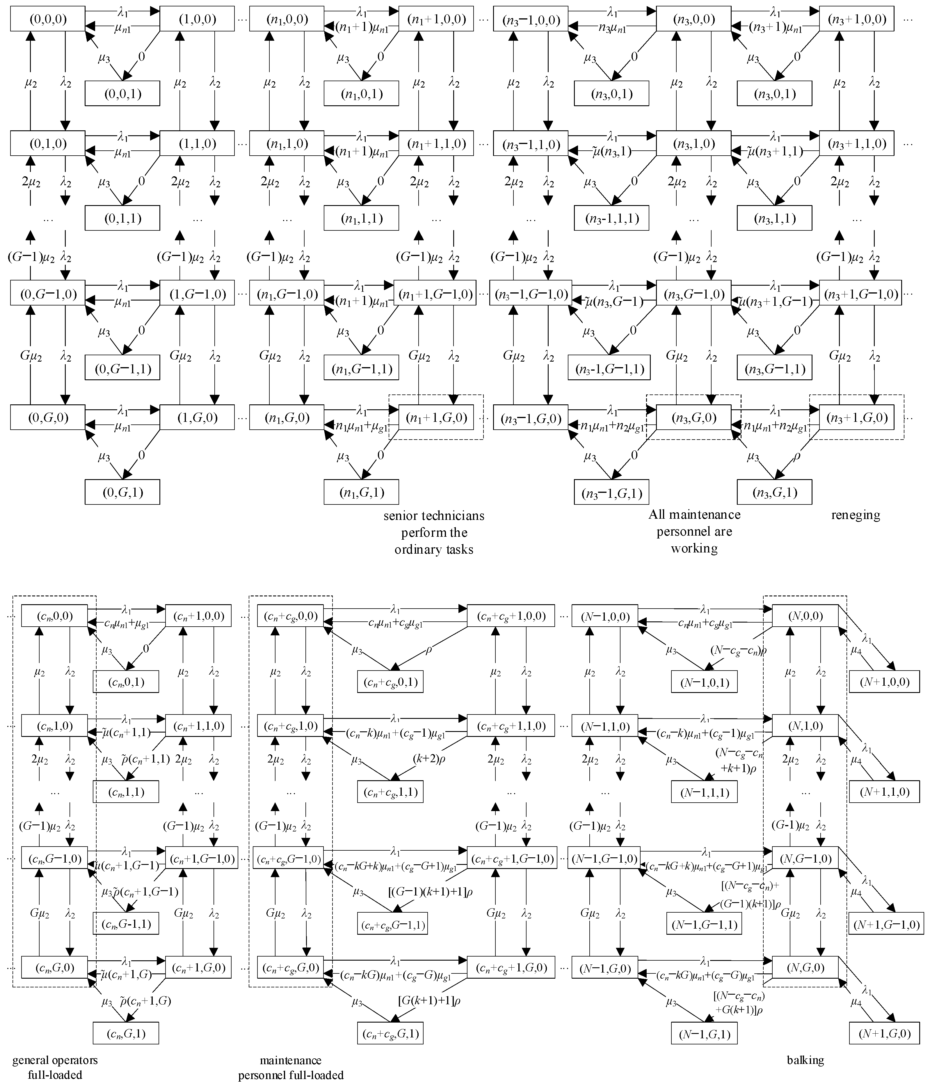
Let us consider (n₃, G, 0) in Figure 1 as an illustrative example to explain the process of state transition, where n₁ = c_n − kG, n₂ = c_g − G and n₃ = n₁ + n₂ with all maintainers currently in operation. Once a special service is completed, a group of maintainers comprising one senior technician and k general operators is released. As a result, the system transitions to (n₃, G − 1, 0). This transition releases k + 1 maintainers. If the number of general operators released exceeds the number of senior technicians currently servicing ordinary customers, i.e., k ≥ n₂, the general operators will take over all the senior technicians’ service for ordinary customers, resulting in a service rate of n₃·μ_n1 for ordinary customers. If k < n₂, only k senior technicians can be replaced, leading to n₁ + k general operators and n₂ − k senior technicians performing ordinary services. The service rate for ordinary customers, in this case, is (n₁ + k)μ_n1 + (n₂ − k)μ_g1. The spatial states are sorted according to a predefined order, and the state transition mechanism of the model is depicted in Figure 1.

Figure 1 illustrates three special states, which are depicted by dashed boxes: (n₁ + 1, G, 0) indicates the state where the first senior technician provides ordinary service; (n₃, G, 0) signifies that all maintainers are currently working, and (n₃ + 1, G, 0) denotes the state where the first ordinary customer reneges due to impatience. The order of these states is determined by the set S.

A state sequence comprises states that share the same value of n and v. There are three sequences that require special attention. The first sequence is the fully loaded sequence of general operators, where the number of ordinary customers in the system is c_n and all the general operators are working. The second sequence is the fully loaded sequence of personnel. In this case, the number of ordinary customers reaches c_n + c_g, and all the maintainers are working. The third sequence is the balking sequence, in which the subsequent ordinary customers will promptly leave the system upon entering once the number of ordinary customers reaches N.

The state transition process related to (n, g, 0) is shown in Figure 2 for the values of n ranging from 1 to N − 1 and g ranging from 1 to G − 1. ${\displaystyle \tilde{\mu }}$ and ${\displaystyle \tilde{\rho }}$ are calculated using Equation (3) and Equation (5), respectively.

The state transition rate matrix of the system can be represented by

$$\begin{array}{ll}\mathit{Q}& ={\left\{q_{i,j}\right\}}_{GT\times GT}\\ & =\left(\begin{array}{ccccccc}{\mathit{A}}_0& {\mathit{C}}_0& & & & & \\ {\mathit{B}}_1& {\mathit{A}}_1& {\mathit{C}}_1& & & & \\ & {\mathit{B}}_2& {\mathit{A}}_2& {\mathit{C}}_2& & & \\ & & \ddots & \ddots & \ddots & & \\ & & & {\mathit{B}}_n& {\mathit{A}}_n& {\mathit{C}}_n& \\ & & & & \ddots & \ddots & \ddots \\ & & & & & {\mathit{B}}_N& {\mathit{A}}_N\end{array}\right)\end{array}$$

(6)

where A_n, B_n, C_n are the submatrices of Q. q_i,j denotes the element in the ith row and the jth column of the transition rate matrix Q.

B_n is the transition rate matrix that represents the reduction of ordinary customers.

$${\mathit{B}}_n={\left\{B_{i,j}^{(n)}\right\}}_{4(G+1)\times (G+1)}, n=1,2,\cdots ,N$$

(7)

where

$$\left\{\begin{array}{l}{B}_{2g+1,2g+1}^{\left(n\right)}=\tilde{\mu }\left(n,g\right)\\ B_{2g+1,2g+2}^{\left(n\right)}=\tilde{\rho }\left(n,g\right)\end{array}\right., g=0,1,2,\cdots ,G$$

(8)

C_n is the transition rate matrix that models the arrival of ordinary customers.

$${\mathit{C}}_n={\left\{C_{i,j}^{\left(n\right)}\right\}}_{4(G+1)\times (G+1)}, n=0,1,2,\cdots ,N-1$$

(9)

where

$$C_{2g+1,2g+1}^{\left(n\right)}={\lambda }_1, g=0,1,2,\cdots ,G$$

(10)

For values of n ranging from 0 to N − 1, A_n is the transition rate matrix between two adjacent state sequences with the same value of n. When n = N, A_N denotes the transition rate matrix between n = N, N + 1, while v = 0.

$${\mathit{A}}_n={\left\{A_{i,j}^{\left(n\right)}\right\}}_{4(G+1)\times (G+1)}, n=0,1,2,\cdots ,N$$

(11)

where i = 2(G + 1)(n − 1)g.

When n = 0, 1, 2,…, N − 1,

$$\left\{\begin{array}{ll}{A}_{2g+2,2g+1}^{\left(n\right)}={\mu }_3\hfill & g=0,1,\cdots ,G\hfill \\ A_{2g+3,2g+1}^{\left(n\right)}=\left(g+1\right){\mu }_2\hfill & g=0,1,\cdots ,G-1\hfill \\ A_{2g+1,2g+3}^{\left(n\right)}={\lambda }_2\hfill & g=0,1,\cdots ,G-1\hfill \\ A_{g,g}^{\left(n\right)}=q_{i,i}\hfill & g=0,1,\cdots ,2\left(G+1\right)\hfill \end{array}\right.$$

(12)

When n = N,

$$\left\{\begin{array}{ll}{A}_{2g+2,2g+1}^{\left(n\right)}={\mu }_4\hfill & g=0,1,\cdots ,G\hfill \\ A_{2g+3,2g+1}^{\left(n\right)}=\left(i+1\right){\mu }_2\hfill & g=0,1,\cdots ,G-1\hfill \\ A_{2g+1,2g+3}^{\left(n\right)}={\lambda }_2\hfill & g=0,1,\cdots ,G-1\hfill \\ A_{2g+1,2g+2}^{\left(n\right)}={\lambda }_1\hfill & g=0,1,\cdots ,G\hfill \\ A_{g,g}^{\left(n\right)}=q_{i,i}\hfill & g=0,1,\cdots ,2\left(G+1\right)\hfill \end{array}\right.$$

(13)

Note that the nondiagonal elements in A_n correspond to the transitions among the 2(G + 1) states, whereas the diagonal element $A_{i,i}^{\left(n\right)}$ represents the Markov process element.

$$A_{i,i}^{\left(n\right)}=q_{i,i}=-{\displaystyle \sum _{j\in \mathit{S},j\ne i}{q}_{i,j}}$$

(14)

4. Steady-State Solution

The steady-state solution of the system comprises the steady-state sojourn probability and the steady-state interstate transition frequency.

4.1. Steady-State Sojourn Probability

Let P(t) = [P₁(t), P₂(t), …, P_GT(t)]^T represent the probability distribution of the system in each state at time t.

$$\left\{\begin{array}{l}{\mathit{P}}^{\prime }\left(t\right)=\mathit{Q}\cdot \mathit{P}\left(t\right)\\ \mathit{P}\left(0\right)={\left(1,\underset{GT-1}{\underbrace{0,0,\cdots ,0}}\right)}^{\mathrm{T}}\end{array}\right.$$

(15)

Applying Laplace transformation to both sides yields the following equation:

$${\mathit{P}}^{*}\left(s\right)={\left(s\mathit{I}-\mathit{Q}\right)}^{-1}\mathit{P}\left(0\right),s>0$$

(16)

where I is an identity matrix. According to Tauberian Theorem,

$$\mathit{P}=\underset{t\to \infty }{\lim }\mathit{P}\left(t\right)=\underset{s\to 0}{\lim }s{\mathit{P}}^{*}\left(s\right)$$

(17)

where P = [P₁, P₂, …, P_GT]^T represents the probabilities of each state in each steady state. These probabilities reflect the sojourn time in each state over a given period.

4.2. Steady-State Interstate Transition Frequency

This paper introduces a novel indicator called the interstate transition frequency, which includes information about both the starting state and entering state. It distinguishes the traditional transition frequency, which only considers the entering state. Let $M_{l,z}^{\left(i\right)}$(t + Δt) denote the number of transitions from state l to state z within the time interval Δt, giving the initial state i. When l ≠ z,

$$M_{l,z}^{\left(i\right)}(t+\Delta t)=\left\{\begin{array}{l}\left[{\displaystyle \sum _{j=1,j\ne z}^{GT}\left(P_{l,j}\left(\Delta t\right)\cdot M_{l,z}^{\left(j\right)}(t)\right)}\right.\\ \left.+P_{l,z}\left(\Delta t\right)\left(1+M_{l,z}^{\left(z\right)}(t)\right)+o\left(\Delta t\right)\right], i=l\\ {\displaystyle \sum _{j=1}^{GT}{P}_{i,j}\left(\Delta t\right)\cdot M_{l,z}^{\left(j\right)}(t)+o\left(\Delta t\right)}\hspace{1em}\hspace{1em}, i\ne l\end{array}\right.$$

(18)

where 1 in the first expression indicates a single transition from state l to z within Δt, denoted as $M_{l,z}^{\left(l\right)}$(Δt) = 1. P_i,j(Δt) represents the probability of the transition from state i to j. This probability can be calculated based on the properties of the exponential distribution and can be expressed as

$$P_{i,j}\left(\Delta t\right)=\left\{\begin{array}{ll}{q}_{i,j}\Delta t& j\ne i\\ 1-{\displaystyle \sum _{j=1,j\ne i}^{GT}{q}_{i,j}\Delta t}& j=i\end{array}\right.$$

(19)

By combining Equation (14) with Equation (19), we simplify the expression as follows:

$$P_{i,j}\left(\Delta t\right)=\left\{\begin{array}{ll}{q}_{i,j}\Delta t& j\ne i\\ 1+q_{i,i}\Delta t& j=i\end{array}\right.$$

(20)

By substituting Equation (20) into Equation (18), one can obtain the following derivation:

$$\frac{M_{l,z}^{\left(i\right)}\left(t+\Delta t\right)-M_{l,z}^{\left(i\right)}\left(t\right)}{\Delta t}=\left\{\begin{array}{ll}{\displaystyle \sum _{j=1}^{GT}{q}_{l,j}\cdot M_{l,z}^{\left(j\right)}(t)+q_{l,z}+\frac{o\left(\Delta t\right)}{\Delta t}}& i=l\\ {\displaystyle \sum _{j=1}^{GT}{q}_{i,j}\cdot M_{l,z}^{\left(j\right)}(t)+\frac{o\left(\Delta t\right)}{\Delta t}}& i\ne l\end{array}\right.$$

(21)

When taking the limit as Δt approaches 0, the right-hand side of Equation (21) converges to a finite value, implying the left-hand side also converges. Therefore, we can conclude that $M_{l,z}^{\left(i\right)}$(t) is differentiable based on this deduction. Furthermore, it is evident from the definition of $M_{l,z}^{\left(i\right)}$(t) that $M_{l,z}^{\left(i\right)}$(0) is equal to 0, where i ∈ S. The matrix representation of Equation (21) is as follows:

$$\left\{\begin{array}{l}{\mathit{M}}_{l,z}^{\prime }\left(t\right)=\mathit{Q}{\mathit{M}}_{l,z}\left(t\right)+{\mathit{W}}_{l,z}\\ {\mathit{M}}_{l,z}\left(0\right)=\mathbf{0}\end{array}\right.$$

(22)

where M_l,z(t) = [$M_{l,z}^{\left(1\right)}$(t), $M_{l,z}^{\left(2\right)}$(t), …, $M_{l,z}^{\left(GT\right)}$(t)]^T; W_l,z = [$W_{l,z}^{\left(1\right)}$, $W_{l,z}^{\left(2\right)}$, …, $W_{l,z}^{\left(GT\right)}$]^T. It should be noted that all elements in W_l,z, except for $W_{l,z}^{\left(l\right)}$ = q_l,z, are equal to 0.

Let $m_{l,z}^{\left(i\right)}$(t) represents the derivative of $M_{l,z}^{\left(i\right)}$(t).

$$m_{l,z}^{\left(i\right)}\left(t\right)=\mathrm{d}{M}_{l,z}^{\left(i\right)}\left(t\right) /\mathrm{d}t ,i\in S$$

(23)

where $m_{l,z}^{\left(i\right)}$(t) represent the transient frequency from state l to z at time t given the initial state i. Apply the Laplace transform to Equation (23).

$$\begin{array}{ll}{m}_{l,z}^{\left(i\right)*}\left(s\right)& ={\displaystyle {\int }_0^{\infty }{e}^{-st}{m}_{l,z}^{\left(i\right)}\left(t\right)\mathrm{d}t}\\ & ={\displaystyle {\int }_0^{\infty }{e}^{-st}\mathrm{d}{M}_{l,z}^{\left(i\right)}\left(t\right)}, s>0\end{array}$$

(24)

One can derive

$$s{\mathit{m}}_{l,z}^{*}\left(s\right)=\mathit{Q}{\mathit{m}}_{l,z}^{*}\left(s\right)+{\mathit{W}}_{l,z}$$

(25)

where ${\mathit{m}}_{l,z}^{*}\left(s\right)={\left[m_{l,z}^{\left(1\right)*}\left(s\right),m_{l,z}^{\left(2\right)*}\left(s\right),\dots ,m_{l,z}^{\left(GT\right)*}\left(s\right)\right]}^{\mathrm{T}}$; that is,

$${\mathit{m}}_{l,z}^{*}\left(s\right)={\left(s\mathit{I}-\mathit{Q}\right)}^{-1}{\mathit{W}}_{l,z}$$

(26)

By applying the Laplace inversion method, we can obtain m_l,z(t). According to the Tauberian Theorem, the steady-state interstate transition frequency m_l,z can be determined as

$${\mathit{m}}_{l,z}=\underset{t\to \infty }{\lim }{\mathit{m}}_{l,z}\left(t\right)=\underset{s\to 0}{\lim }s{\mathit{m}}_{l,z}^{*}\left(s\right)$$

(27)

According to the steady-state properties, m_l,z is independent of the initial state, resulting in the elements in the column vector m_l,z being the same. The subsequent sections exclusively focus on steady-state analysis. For simplicity, we express $m_{l,z}^{\left(i\right)}$ without explicitly stating (i), and this can be given by

$$m_{l,z}=m_{l,z}^{\left(i\right)},i\in \mathit{S}$$

(28)

According to the properties of the Markov process, two state transitions cannot occur within Δt. Hence, in the case l = z, m_z,z = 0.

5. System Operation Indicators

By building upon the models of Kim [24] and Vasiliadis [25], we propose the following performance indicators.

5.1. Critical Interstate Transition Frequency

The transition frequencies between critical states play a crucial role in system operation indicators, primarily encompassing the service frequency and the abandonment frequency.

(1)

Frequency of ordinary service L_n

$$L_n={\displaystyle \sum _{g=0}^G{\displaystyle \sum _{n=0}^{N-1}{m}_{2\left(G+1\right)\left(n+1\right)+2g+1,2\left(G+1\right)n+2g+1}}}$$

(29)

(2)

Frequency of special service L_g

$$L_g={\displaystyle \sum _{g=0}^{G-1}{\displaystyle \sum _{n=0}^N{m}_{2\left(G+1\right)n+2g+3,2\left(G+1\right)n+2g+1}}}$$

(30)

From Equations (29) and (30), it is observed that the entering states are identical. When the starting state is indistinguishable, it becomes impossible to determine the specific level of the service that has been completed. Therefore, interstate transition frequency, which quantifies the frequency of transitions between states, becomes more meaningful than the traditional transition frequency.

(3)

Reneging frequency L_r

When n > l_n + l_g, indicating a lack of workforce, the ordinary customers who cannot be serviced in time will renege. In such instances, when a customer reneges, the system state transitions from (n, g, 0) to (n − 1, g, 1) and instantaneously from (n − 1, g, 1) to (n − 1, g, 0) due to μ₃→∞. By calculating the frequency of the transition from (n − 1, g, 1) to (n − 1, g, 0), one can obtain L_r:

$$L_r={\displaystyle \sum _{g=0}^G{\displaystyle \sum _{n=l_n+l_g+1}^N{m}_{2\left(G+1\right)n+2g+1,2\left(G+1\right)\left(n-1\right)+2g+2}}}$$

(31)

Since μ₃→∞, the system’s duration in (n − 1, g, 1) approaches 0, which indicates that the probability of being in that state at any given time tends to zero. Consequently, employing the sojourn probability to count the number of reneging is not feasible. However, Equation (31) reveals that the frequency of reneging can be effectively addressed by interstate transition frequency. Therefore, interstate transition frequency offers greater flexibility in calculating system indicators compared to state sojourn probability. This advantage is also reflected in the formulation of the balking frequency.

(4)

Balking frequency L_b

When the number of ordinary customers reaches N, and an additional ordinary customer arrives, the system state transitions from (N, g, 0) to (N + 1, g, 0) and then immediately reverts to (N, g, 0) due to assumption 4). L_b can be determined by calculating the transition frequency from (N + 1, g, 0) to (N, g, 0).

$$L_b={\displaystyle \sum _{g=0}^G{m}_{2\left(G+1\right)N+2g+2,2\left(G+1\right)N+2g+1}}$$

(32)

5.2. Waiting Time Analysis

The waiting time T_d represents the cumulative waiting time of all customers throughout the system’s operation interval T_s. In order to accurately reflect this, it is important to consider the sojourn time in each state as well as the number of waiting customers in the corresponding state. Additionally, capturing the reasons for state transitions during the system operation allows T_d to be categorized into four distinct parts.

$$T_d=T_{d1}+T_{d2}+T_{d3}+T_{d4}$$

(33)

(1)

T_d1 represents the waiting time caused by ordinary services. During this time, the system transitions from (n, g, 0) to (n − 1, g, 0) is

$$T_{d1}=T_s{\displaystyle \sum _{g=0}^G{\displaystyle \sum _{n=l_n+l_g+1}^{N}y{P}_{i,j}}}$$

(34)

where i = 2(G + 1)n + 2g + 1, j = 2(G + 1)(n − 1) + 2g + 1.

(2)

T_d2 represents the waiting time caused by special services. During this time, the system transitions from (n, g, 0) to (n, g − 1, 0) is

$$T_{d2}=T_s{\displaystyle \sum _{g=0}^{G-1}{\displaystyle \sum _{n=l_n+l_g+1}^{N}y{P}_{i,j}}}$$

(35)

where i = 2(G + 1)n + 2g + 3, j = 2(G + 1)n + 2g + 1.

(3)

T_d3 represents the waiting time caused by reneging. The transition occurs from (n, g, 0) to (n − 1, g, 1), then transits to (n − 1, g, 0). However, as μ₃→∞, the state transitions to (n − 1, g, 0) instantaneously, making the transition time negligible.

$$T_{d3}=T_s{\displaystyle \sum _{g=0}^G{\displaystyle \sum _{n=l_n+l_g+1}^{N}y{P}_{i,j}}}$$

(36)

where i = 2(G + 1)n + 2g + 1, j = 2(G + 1)(n − 1) + 2g + 2.

(4)

T_d4 represents the waiting time due to balking. The system transitions from (N, g, 0) to (N + 1, g, 0), and as μ₄→∞, it returns to (N, g, 0) immediately.

$$T_{d4}=T_s{\displaystyle \sum _{g=0}^G\left(N-l_n-l_g\right)P_{i,j}}$$

(37)

where i = 2(G + 1)N + 2g + 1, j = 2(G + 1)N + 2g + 2.

The meaning of Equations (33)–(37) is as follows: T_s∙P_i,j represents the sojourn time at state i before transitioning to state j during the system’s runtime. This time is then multiplied by the number of waiting customers y to obtain the waiting time at each state. Finally, the waiting time for the corresponding state is summed, considering the different reasons for the transitions.

5.3. Working Time Analysis

It is known to all that a maintainer should not be continuously occupied during runtime. Hence, it is reasonable to establish a correlation between wages and working intensity. In order to calculate the working intensity P_lw for two-level maintainers, it is crucial to compute the corresponding working time T_l individually. T_l is influenced by both the steady-state sojourn probability and the number of maintainers at the same level.

$$T_l=\frac{T_{lg}+T_{ln}}{c_l}=\frac{T_s}{c_l}{\displaystyle \sum _{n=1}^N{\displaystyle \sum _{g=0}^G\left(w_{lg}+w_{ln}\right)P_i}}$$

(38)

where T_l denotes the average working time for level l, l = g, n, representing senior technicians and general operators, respectively. T_lg and T_ln represent the total working time of level l maintainers servicing special and ordinary customers, respectively. i = (2G + 1)n + 2g + 1.

Accordingly, the actual working intensity, denoted as P_lw, can be expressed as

$$P_{lw}=\frac{T_l}{T_S}$$

(39)

5.4. Operation Profit Analysis

Referring to the utilization of Markov process in networks [26] and queuing theory in hospitals [27], a comprehensive profit analysis is performed.

The profit of the system can be calculated based on the system parameters k, c_n, c_g, and N. By taking profit as the objective function, the system parameters can be optimized. The details of operation profit are as follows:

(1)

The income of the system per unit of time is divided into two parts: the income from ordinary customers (L_nC_n), which is derived from the frequency of ordinary customers and the income per ordinary customer, and the income from special customers (L_gC_g), which is calculated by multiplying the frequency of special customer by the income per special customer;

(2)

The cost of abandonment per unit of time is composed of two parts. One is the number of reneging customers per unit of time and the cost per reneging customer, denoted as L_rC_r. The other is calculated by the number of balking customers per unit of time and the cost per balking customer, denoted as L_bC_b;

(3)

The waiting cost, denoted as T_dC_d, is calculated by multiplying the waiting time by the cost per unit of time of waiting;

(4)

The wages of maintenance personnel are determined through a floating mechanism according to P_gw and P_nw. The personnel cost, denoted as C_w, can be expressed as

$$C_w=\frac{T_s}{T_w}{\displaystyle \sum _{l=n,g}{S}_l\left(P_{lw}\right)}$$

(40)

where S_l(P_lw) denotes the weekly wages of class l, and T_w is the weekly business time.

It should be noted that this paper studies the system configuration before the actual operation. It assumes that service rates for different levels of maintainers are constant, ensuring that there are no intentional service delays due to wages.

(5)

The site cost is calculated as (N + G)C_N. N and G are the capacities of ordinary customers and special customers, respectively. C_N is the cost of a single space.

Therefore, the total profit of the system C can be calculated as:

$$C=T_s\left(L_n{C}_n+L_g{C}_g-L_a{C}_a-L_e{C}_e\right)-T_d{C}_d-C_w-\left(N+G\right)C_N$$

(41)

6. Numerical Example

An automobile repair shop is considered here as an illustrative example. The repair shop primarily offers two types of services: vehicle maintenance and repair. The staff includes c_n general operators and c_g senior technicians, and each maintenance work is assigned to a single maintainer. When a car requires a repair, the customer is granted pre-emptive priority. The repair progress is promptly handled by k general operators and one senior technician, with greater values of k equating to increased efficiency. Generally, k is chosen from the set {1, 2, 3} due to spatial limitations. In cases of insufficient manpower, some maintainers may temporarily cease ongoing maintenance to prioritize repair services. Maintenance services typically favor general operators. In order to ensure repair service priority and consider working site constraints, the repair shop can only simultaneously accommodate G vehicles for repair and N vehicles for maintenance. For the sake of controlling the system scale while maintaining generality, we set G = 2.

The arrival interval and service time of vehicles in the system follow exponential distributions. The average arrival interval for maintenance vehicles is 40 min, whereas it is 200 min for repair vehicles. A senior technician requires an average maintenance time of 200 min per vehicle, whereas a general operator needs 240 min per vehicle. The average repair times per vehicle for k = 1, 2, and 3 are 360, 330, and 300 min, respectively. The maintenance vehicles waiting in the system will renege with an exponential distribution of 120 min per vehicle. The average duration of both abandonment and barking is 1 s.

The repair shop earns USD 1000 per vehicle for maintenance work and USD 5000 per vehicle for repair work. The waiting cost is USD 10 per minute. The shop incurs a loss of USD 1000 per vehicle when a customer reneges and USD 2500 per vehicle when balking occurs. The site cost for each working space is USD 2500 per month. The weekly wages of personnel vary based on the actual work intensity. The weekly business time, denoted as T_w, is calculated as T_w = 5 × 8 × 60 = 2400 (min). The specific allocation scheme of wages can be found in

Table 1. Details of wages according to fluctuating mechanism S_l(p_lw).

Senior Technicians		General Operators
Weekly Wages Cg (USD/Person)	Working Intensity Pgw	Weekly Wages Cn (USD/Person)	Working Intensity Pnw
1500	[0, 40%)	1000	[0, 60%)
2000	[40%, 60%)	1250	[60%, 70%)
2500	[60%, 100%)	1500	[70%, 100%)

.

Then, the system parameters k, c_n, c_g, and N can be determined by optimizing the profit of the shop.

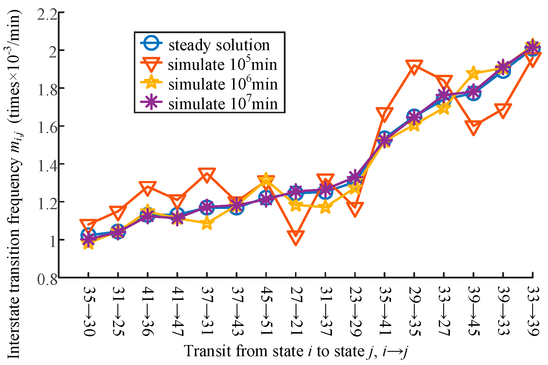
6.1. Comparison of Interstate Transition Frequency between Theory and Simulation

In order to verify the theoretical calculation of interstate transition frequency, the MCMC (Markov chain Monte Carlo) method is employed. The system with parameters k = 2, c_n = 6, c_g = 3, and N = 10 was selected, and we compared several frequencies of interstate transition that were more likely to occur. The results are demonstrated in Figure 3.

As can be seen from Figure 3, it is evident that the simulation results gradually approach the theoretical results as the simulation runtime increases. At a runtime of 10⁶ min (8.7 years), the simulation results are closely aligned with the theoretical results. Moreover, as the system reaches 10⁷ min, the two curves nearly coincide, indicating that the system has reached a steady state. Thus, the proposed method is demonstrated to be valid.

6.2. Analysis of Optimization

In order to calculate the system’s profit, we consider a month-long period consisting of 20 days and 8 h per day, resulting in T_s = 20 × 8 × 60 = 9600 (min). The maximum system profit is then determined for various combinations of k and N, and the results are presented in Figure 4.

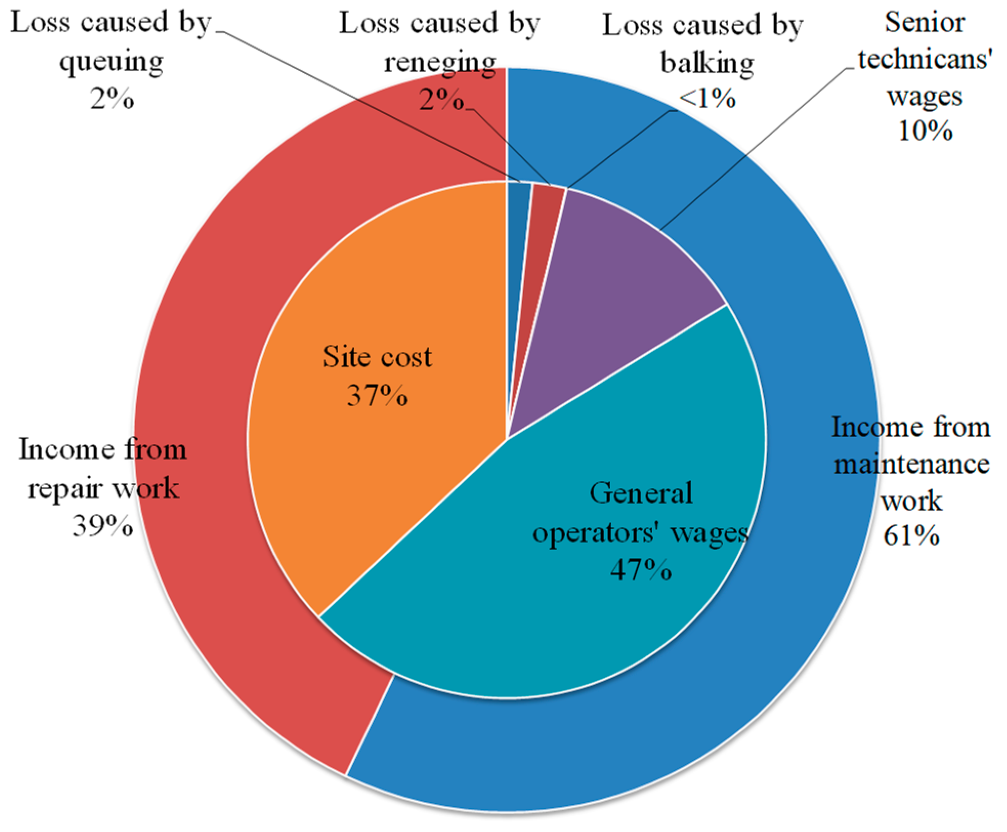
The results displayed in Figure 4 indicate that the maximum profit initially increases and then decreases as ordinary customer capacity N increases. An obvious gradual trend is observed when N ≥ 14. Specifically, when k = 3, c_n = 15, c_g = 2, and N = 17, the system achieves a maximum profit of USD 287,000. The proportion of income and cost in each part is shown in Figure 5.

Figure 5 depicts the income and cost of the system, which are represented by the outer and inner circles, respectively. The total income is USD 415,000, whereas the total cost amounts to USD 128,000.

The repair shop handles an average of 35.63 vehicle repairs and 237.27 vehicle maintenances each month. The majority of the income, 61%, is generated from maintenance services.

The system experiences a relatively high proportion of costs from the personnel and site, constituting 57% and 37%, respectively. Among the personnel expenses, ordinary operators have a working intensity of 58.08%, resulting in weekly wages of USD 2000 per person, according to Table 1. Similarly, the senior technicians have a working intensity of 46.55%, and their weekly wages are also set at USD 2000 per person.

It is noteworthy that the losses attributed to waiting and reneging account for 2% each, and the loss due to balking is less than 1%. These numbers indicate that customers receive satisfactory service under the current configuration. The total waiting time for maintenance vehicles is 205.8 min, resulting in an average waiting time of less than 1 min. Furthermore, the monthly number of reneging vehicles is 2.71, and the number of balking vehicles is 0.01, both of which can be considered marginal.

7. Conclusions

This study focuses on the analysis of a queuing system model that integrates multiple priorities, multiple abandonments, and heterogeneous servers. The model was solved and optimized by employing the combination of the Markov process with block matrix theory. The findings of this study are summarized as follows.

(1)

A novel system indicator called interstate transition frequency is introduced. In the context of CTMC, interstate transition frequency is proposed as the new computational target, replacing the sojourn probability. This substitution is based on the ability of interstate transition frequency to decompose the sojourn probability. Consequently, the transitions with the same entering state can be distinguished during the evolution process. In order to accurately simulate the abandonment process, a non-sojourn state is introduced in the CTMC framework, and this process can only be described by using the new indicator;

(2)

Based on interstate transition frequency, several system operation indicators are obtained, including service frequency, reneging frequency, balking frequency, total waiting time, and system profit. These indicators significantly enhance the evaluation methodology for queuing systems with multiple priority, multiple abandonments, and heterogeneous servers;

(3)

The proposed queuing model was implemented in an automobile repair shop. The accuracy of interstate transition frequency was validated. The shop configuration was optimized, with a focus on maximizing system profit. Based on the optimization results, a succinct financial report is provided.