Novel Multistep Implicit Iterative Methods for Solving Common Solution Problems with Asymptotically Demicontractive Operators and Applications

Abstract

It is very meaningful and challenging to efficiently seek common solutions to operator systems (CSOSs), which are widespread in pure and applied mathematics, as well as some closely related optimization problems. The purpose of this paper is to introduce a novel class of multistep implicit iterative algorithms (MSIIAs) for solving general CSOSs. By using Xu’s lemma and Maingé’s fundamental and important results, we first obtain strong convergence theorems for both one-step and multistep implicit iterative schemes for CSOSs, involving asymptotically demicontractive operators. Finally, for the applications and profits of the main results presented in this paper, we give two numerical examples and present an iterative approximation to solve the general common solution to the variational inequalities and operator equations.

1. Introduction

Throughout this paper, let $\mathcal{H},{\mathcal{H}}_1$, and ${\mathcal{H}}_2$ be three real Hilbert spaces with the inner product as $\langle ·,·\rangle$, and the induced norm as $\parallel ·\parallel$. Assume that ${\mathsf{ȷ}}_1:=\{1,2,\cdots ,p_1\}$ and ${\mathsf{ȷ}}_2:=\{1,2,\cdots ,p_2\}$ are two sets; here, $p_1$ and $p_2$ are two arbitrary positive integers. We assume that all the problems and iterative schemes are well-defined.

For all $i\in {\mathsf{ȷ}}_1$ and each $j\in {\mathsf{ȷ}}_2$, let $S_i:\mathcal{H}\to \mathcal{H}$ and $F_j:\mathcal{H}\to \mathcal{H}$ be two nonlinear operators, and $Q_j\subset \mathcal{H}$ be a given nonempty closed convex subset for any $j\in {\mathsf{ȷ}}_2$. In order to solve the general common solution to variational inequalities and operator equations (GCSVIOE), we consider the following:

$$\left\{\begin{array}{c}0=x-S_{i}x,\forall i\in {\mathsf{ȷ}}_1,\hfill \\ \langle F_{j}x,y_j-x\rangle \ge 0,\forall y_j\in Q_j,j\in {\mathsf{ȷ}}_2.\hfill \end{array}\right.$$

(1)

It is not difficult to note that (1) can also be reformulated as the following nonlinear operator system (see [1]):

$$\left\{\begin{array}{c}0=x-S_{i}x,\forall i\in {\mathsf{ȷ}}_1,\hfill \\ 0=x-P_{Q_j}(I-\rho F_j)x,\forall j\in {\mathsf{ȷ}}_2,\hfill \end{array}\right.$$

(2)

where $\rho$ is a positive constant, I is the identity operator, and for each $j\in {\mathsf{ȷ}}_2$, $P_{Q_j}$ is the metric projection from $\mathcal{H}$ to $Q_j$, which is used to find the unique point $P_{Q_j}x$ in $Q_j$ fulfilling

$$\parallel x-P_{Q_j}x\parallel =inf\left\{\parallel x-y\parallel |y\in Q_j\right\},$$

i.e.,

$$\langle x-P_{Q_j}x,y-P_{Q_j}x\rangle \le 0,\forall y\in Q_j.$$

If $P_{Q_j}(I-\rho F_j)$ in (2) is generally replaced by $T_j:\mathcal{H}\to \mathcal{H}$ for all $j\in {\mathsf{ȷ}}_2$, then one can easily see that GCSVIOE is a special case of the following common solution problem for the operator system (CSOS) involved in the nonlinear operators $S_i$ and $T_j$, which aims to locate the point $x\in \mathcal{H}$ such that

$$\left\{\begin{array}{c}0=x-S_{i}x,\forall i\in {\mathsf{ȷ}}_1,\hfill \\ 0=x-T_{j}x,\forall j\in {\mathsf{ȷ}}_2.\hfill \end{array}\right.$$

(3)

Example 1.

When ${\mathsf{ȷ}}_1$ and ${\mathsf{ȷ}}_2$ are single point sets, i.e., $p_k=1$ for $k=1,2$, and $S_1$ and $T_1$ are separately denoted as S and T, one has the following special nonlinear operator system from (3):

$$0=x-Sx\mathrm{and}0=x-Tx.$$

(4)

Example 2.

If $T_j=I$ for every $j\in {\mathsf{ȷ}}_2$, then (3) reduces to a family of operator equations as follows:

$$\begin{array}{ccc}\hfill & & (I-S_i)x=0,\forall i\in {\mathsf{ȷ}}_1,\hfill \end{array}$$

(5)

which was considered by Gu and He [2].

Furthermore, the split common fixed point problem (SCFPP), which is used to describe intensity-modulated radiation therapy, can be transformed into a CSOS.

Example 3.

Give a bounded linear operator $A:{\mathcal{H}}_1\to {\mathcal{H}}_2$, and two series of nonlinear operators $S_i:{\mathcal{H}}_1\to {\mathcal{H}}_1$ for any $i\in {\mathsf{ȷ}}_1$ and $T_j:{\mathcal{H}}_2\to {\mathcal{H}}_2$ for each $j\in {\mathsf{ȷ}}_2$. Then, the SCFPP can be formulated by finding the point $(x_1,x_2)\in ({\mathcal{H}}_1,{\mathcal{H}}_2)$ such that

$$\left\{\begin{array}{c}A{x}_1=x_2,\hfill \\ x_1=S_i{x}_1,\forall i\in {\mathsf{ȷ}}_1,\hfill \\ x_2=T_j{x}_2,\forall j\in {\mathsf{ȷ}}_2,\hfill \end{array}\right.$$

which was first introduced by Censor and Segal [3] in 2009 and has attracted widespread attention—see [4]. According to the Lemma 3.2 in [5], the SCFPP can be transformed into the following CSOS: Find $x\in {\mathcal{H}}_1$ such that

$$\left\{\begin{array}{c}0=x-S_{i}x,\forall i\in {\mathsf{ȷ}}_1,\hfill \\ 0=x-{\left(A^{*}A\right)}^{-1}{A}^{*}{T}_{j}Ax,\forall j\in {\mathsf{ȷ}}_2,\hfill \end{array}\right.$$

where $A^{*}$ is the adjoint operator of A.

Remark 1.

We remark that CSOSs have a wide range of applications in physics [6], mechanics [7], control theory [8], economics [9], information science [10], and other problems in pure and applied mathematics and some highly related optimization problems [11,12].

In order to solve (5), Gu and He [2] introduced the following multistep iterative process with errors $u_n^{\left(i\right)}$ for $i\in {\mathsf{ȷ}}_1$ and $n\in \mathbb{N}$:

$$\left\{\begin{array}{c}{x}_1\in C,\hfill \\ x_{n+1}=x_n^{\left(0\right)},\hfill \\ x_n^{(i-1)}=a_n^{\left(i\right)}{S}_i{x}_n^{\left(i\right)}+b_n^{\left(i\right)}{x}_n+c_n^{\left(i\right)}{u}_n^{\left(i\right)},\hfill \\ x_n^{\left(p_1\right)}=x_n,\hfill \end{array}\right.$$

(6)

where C is a nonempty closed convex subset of $\mathcal{H}$ and $S_i:C\to C$. $\left\{a_n^{\left(i\right)}\right\},\left\{b_n^{\left(i\right)}\right\}$ and $\left\{c_n^{\left(i\right)}\right\}$ are three real sequences in $[0,1]$ and satisfy certain conditions. They also prove that (6) converges strongly to a common solution while ${\left\{S_i\right\}}_{i\in {\mathsf{ȷ}}_1}$ is a family of nonexpansive operators in Banach space. Afterward, when $S_i$ in (5) is the more general asymptotically demicontractive operator for all $i\in {\mathsf{ȷ}}_1$, Wang et al. [13] introduced an iteration scheme as follows:

$$\left\{\begin{array}{c}{x}_1\in \mathcal{H},\hfill \\ x_{n+1}=(1-a_n-b_n)x_n+b_n\sum _{i=1}^{p_1}{c}_i{S}_i^n{x}_n,\forall n\in \mathbb{N},\hfill \end{array}\right.$$

(7)

where $\left\{a_n\right\}$, $\left\{b_n\right\}\subset (0,1)$ are two real sequences, and a strong convergence theorem was also obtained in real Hilbert space.

In order to solve (3), which is involved in a family of nonexpansive operators ${\left\{S_i\right\}}_{i\in \mathsf{ȷ}}$ and a series of asymptotically nonexpansive operators ${\left\{T_j\right\}}_{j\in \mathsf{ȷ}}$, here, when $\mathsf{ȷ}=\{1,2,\cdots ,k\}$ and $k\in \mathbb{N}$, Yolacan and Kiziltunc [14] proposed the following multistep approximation algorithm (YKMSA):

$$\left\{\begin{array}{c}{x}_1\in \mathcal{H},\hfill \\ x_{n+1}=x_n^{\left(k\right)},\hfill \\ x_n^{\left(i\right)}=a_n^{\left(i\right)}{T}_i^n{x}_n^{(i-1)}+b_n^{\left(i\right)}{S}_i{x}_n+c_n^{\left(i\right)}{u}_n^{\left(i\right)},\hfill \\ x_n^{\left(0\right)}=x_n.\hfill \end{array}\right.$$

(8)

On the other hand, it is well known that the implicit rule is one powerful tool in the field of ordinary differential equations and is widely used to construct the iteration scheme for (asymptotically) nonexpansive-type operators; see, for example, [15,16,17,18,19] and the references therein. Of particular note is that Aibinu and Kim [20] compared the convergence rates of the following two viscosity implicit iterations:

$$\left\{\begin{array}{c}{x}_1\in \mathcal{H},\hfill \\ x_{n+1}=a_{n}S{x}_n+(1-a_n)T(b_n{x}_n+(1-b_n)x_{n+1}),\forall n\ge 1,\hfill \end{array}\right.$$

(9)

and

$$\left\{\begin{array}{c}{x}_1\in \mathcal{H},\hfill \\ x_{n+1}=a_{n}S{x}_n+b_n{x}_n+c_{n}T(d_n{x}_n+(1-d_n)x_{n+1}),\forall n\ge 1,\hfill \end{array}\right.$$

(10)

where $\left\{a_n\right\},\left\{b_n\right\},\left\{c_n\right\}$, and $\left\{d_n\right\}$ are four sequences satisfied by special conditions, and S and T are two self operators for $\mathcal{H}$. They also proved that iteration (10) converges faster than (9) under some prerequisites.

Due to the complexity and effectiveness of the implicit rules (see [19]), there are few pieces of research on implicit iterations for the more general asymptotically demicontractive operators. Thus, the following question comes naturally:

Question 1.

How can a novel iteration scheme be to established with an implicit rule for the CSOSs (3) involved in asymptotically demicontractive operators? What conditions should be satisfied for strong convergence?

Motivated and inspired by the above-mentioned works, we provide a kind of novel multistep implicit iteration algorithm (MSIIA) to answer Question 1. The basic definitions of the related nonlinear operators and some useful lemmas are given in Section 2. In Section 3, we present the details of the proposed MSIIA and prove the main results. Two numerical experiments and an application on GCSVIOE are shown in Section 4. Finally, we make a brief summary of this paper in Section 5. Our studies extend and generalize the results of Gu and He [2], Wang et al. [13], and Yolacan and Kiziltunc [14].

2. Preliminary

In a real Hilbert space $\mathcal{H}$, the following inequalities hold for all $x,y\in \mathcal{H}$:

$$\begin{array}{c}\hfill {\parallel x+y\parallel }^2\le {\parallel x\parallel }^2+2\langle y,x+y\rangle ,\end{array}$$

(11)

and

$$\begin{array}{c}\hfill {\parallel ax+(1-a)y\parallel }^2\le {a\parallel x\parallel }^2+(1-a){\parallel y\parallel }^2,\forall a\in [0,1].\end{array}$$

(12)

In the remainder of this section, we recall some useful definitions and lemmas.

Definition 1.

A nonlinear operator $U:\mathcal{H}\to \mathcal{H}$ with fixed point set $Fix\left(U\right)\ne Ø$ is said to be

(i)

a $c$—contraction if there exists a constant $c\in [0,1)$ such that

$$\begin{array}{c}\hfill \parallel Ux-Uy\parallel \le c\parallel x-y\parallel ,\forall x,y\in \mathcal{H};\end{array}$$

(ii)

nonexpansive if

$$\begin{array}{c}\hfill \parallel Ux-Uy\parallel \le \parallel x-y\parallel ,\forall x,y\in \mathcal{H};\end{array}$$

(iii)

L-Lipschitzian-continuous if there exists a constant $L\ge 0$ such that

$$\begin{array}{c}\hfill \parallel Ux-Uy\parallel \le L\parallel x-y\parallel ,\forall x,y\in \mathcal{H};\end{array}$$

(iv)

L-uniformly Lipschitzian-continuous if there exists a constant $L\ge 0$ such that

$$\begin{array}{c}\hfill \parallel U^{n}x-U^{n}y\parallel \le L\parallel x-y\parallel ,\forall x,y\in \mathcal{H};\end{array}$$

(v)

δ-demicontractive if there exists a constant $\delta \in [0,1)$ such that

$$\begin{array}{c}{\parallel Ux-p\parallel }^2\le {\parallel x-p\parallel }^2+\delta {\parallel Ux-x\parallel }^2,\forall x\in \mathcal{H}andp\in Fix\left(U\right),\end{array}$$

which is also equivalent to

$$\begin{array}{ccc}\hfill \langle x-Ux,x-p\rangle & \ge & \frac{1-\delta }{2}{\parallel x-Ux\parallel }^2;\hfill \end{array}$$

(vi)

asymptotically demicontractive if there exists a sequence $\left\{k_n\right\}\subset [0,\infty )$ with ${lim}_{n\to \infty }{k}_n=1$ and a constant $\kappa \in [0,1)$ such that

$$\begin{array}{c}\hfill \parallel U^n{x-q\parallel }^2\le k_n^2{\parallel x-q\parallel }^2+\kappa {\parallel x-U^{n}x\parallel }^2,\forall x\in C,q\in F\left(U\right),\end{array}$$

which is also equivalent to the following inequalities:

$$\begin{array}{ccc}& & \langle U^{n}x-q,x-q\rangle \le \frac{k_n^2+1}{2}{\parallel x-q\parallel }^2+\frac{\kappa -1}{2}{\parallel x-U^{n}x\parallel }^2,\hfill \\ & & \langle U^{n}x-x,x-q\rangle \le \frac{k_n^2-1}{2}{\parallel x-q\parallel }^2+\frac{\kappa -1}{2}{\parallel x-U^{n}x\parallel }^2.\hfill \end{array}$$

In order to enhance clarity and precision, we use a $(k_n,\kappa )$-asymptotically demicontractive operator to represent the above-defined asymptotically demicontractive operator for the sake of convenience.

Lemma 1 

([21]). Let C be a nonempty closed convex subset of $\mathcal{H}$ and $U:C\to C$ be a L-uniformly Lipschitzian-continuous and asymptotically demicontractive operator. Then, $Fix\left(U\right)$ is a closed convex subset of C.

Definition 2.

Let $U:\mathcal{H}\to \mathcal{H}$ be an operator. Then, $I-U$ is noted as being demiclosed at zero if, for any $\left\{x_n\right\}\subset \mathcal{H}$, the following implication holds:

$$\begin{array}{ccc}\hfill \left.\begin{array}{c}\hfill x_n\rightharpoonup x\\ \hfill (I-U)x_n\to 0\end{array}\right\}& \Rightarrow & x=Ux,\hfill \end{array}$$

where ⇀ and → represent weak and strong convergence, respectively.

Definition 3 

([22]). An operator $T:\mathcal{H}\to \mathcal{H}$ is called uniformly asymptotically regular if, for any bounded subset C of $\mathcal{H}$, there is the following equality:

$$\underset{n\to \infty }{lim}\underset{x\in C}{sup}\parallel T^{n+1}x-T^{n}x\parallel =0.$$

Example 4 

([23]). Let $K=\mathbb{R}$, and $T:K\to K$ be defined by

$$T\left(x\right)=\left\{\begin{array}{cc}rx,\hfill & if0\le x\le 1/2,\hfill \\ {\displaystyle \frac{r(r-x)}{2r-1}},\hfill & if1/2\le x\le r,\hfill \\ 0,\hfill & ifx<0\mathrm{or}x>r,\hfill \end{array}\right.$$

(13)

where $1/2<r<1$ is a given constant. Then, T is a uniformly Lipschitzian-continuous and a $(r,0)$-asymptotically demicontractive operator that is uniformly asymptotically regular for K, and $I-T$ is demiclosed at 0. The fixed point of T is 0.

Example 5.

Let C be a nonempty closed convex subset of $\mathcal{H}$, and operator $F:C\to \mathcal{H}$ be a $\sigma /{\mu }^2$-inverse strongly monotone operator, i.e., $\sigma /{\mu }^2{\parallel Fx-Fy\parallel }^2\le \langle Fx-Fy,x-y\rangle$ for any $x,y\in C$. Then, $T:=P_C(I-\rho F)$ is uniformly asymptotically regular if constant $\rho \in (0,2\sigma /{\mu }^2)$.

Proof. 

Since F is $\sigma /{\mu }^2$-inverse strongly monotone, F is also $\mu$-Lipschitizan-continuous and $\sigma$-strongly monotone such that ${\sigma \parallel x-y\parallel }^2\le \langle Fx-Fy,x-y\rangle$.

Now, we have the following inequality for all $z\in C$:

$$\begin{array}{ccc}& & \parallel T^{n+1}z-T^n{z\parallel }^2\hfill \\ & & =\parallel {\left[P_C(I-\rho F)\right]}^{n+1}z-{\left[P_C(I-\rho F)\right]}^n{z\parallel }^2\hfill \\ & & \le \parallel (I-\rho F)T^{n}z-(I-\rho F)T^{n-1}{z\parallel }^2\hfill \\ & & \le \parallel (T^{n}z-T^{n-1}z)-\rho (F{T}^{n}z-F{T}^{n-1}z){\parallel }^2\hfill \\ & & =\parallel T^{n}z-T^{n-1}{z\parallel }^2-2\rho \langle T^{n}z-T^{n-1}z,F{T}^{n}z-F{T}^{n-1}z\rangle +{\rho }^2{\parallel F{T}^{n}z-F{T}^{n-1}z\parallel }^2\hfill \\ & & \le \parallel T^{n}z-T^{n-1}{z\parallel }^2+({\rho }^2-2\rho \frac{\sigma }{{\mu }^2}){\parallel F{T}^{n}z-F{T}^{n-1}z\parallel }^2\hfill \\ & & =(1+{\rho }^2{\mu }^2-2\rho \sigma ){\parallel T^{n}z-T^{n-1}z\parallel }^2\hfill \\ & & \le {(1+{\rho }^2{\mu }^2-2\rho \sigma )}^n{\parallel Tz-z\parallel }^2.\hfill \end{array}$$

It follows from $\rho \in (0,2\sigma /{\mu }^2)$ that

$$\begin{array}{c}\hfill \underset{n\to \infty }{lim}\underset{z\in C}{sup}\parallel T^{n+1}z-T^{n}z\parallel \le \underset{n\to \infty }{lim}\underset{z\in C}{sup}{(1+{\rho }^2{\mu }^2-2\rho \sigma )}^{\frac{n}{2}}\parallel Tz-z\parallel =0,\end{array}$$

which means that T is uniformly asymptotically regular.    □

Lemma 2 

([24]). Let $\left\{{\mathrm{\Psi }}_n\right\}$ be a sequence of nonnegative real numbers such that

$${\mathrm{\Psi }}_{n+1}\le (1-a_n){\mathrm{\Psi }}_n+a_n{b}_n,n\in \mathbb{N},$$

where $\left\{a_n\right\}$ and $\left\{b_n\right\}$ satisfy the following conditions:

(i)

$a_n\in [0,1]$ and ${\sum }_{n=0}^{\infty }{a}_n=\infty$; (ii)${lim\; sup}_{n\to \infty }{b}_n\le 0$.

Then, ${lim}_{n\to \infty }{\mathrm{\Psi }}_n=0$.

Lemma 3 

([25]). Suppose that $\left\{{\mathrm{\Psi }}_k\right\}$ is a real number sequence that does not decrease at infinity. Then, there exists a subsequence ${\left\{{\mathrm{\Psi }}_{k_j}\right\}}_{j\ge 0}$ of $\left\{{\mathrm{\Psi }}_k\right\}$ such that

$${\mathrm{\Psi }}_{k_j}<{\mathrm{\Psi }}_{k_j+1}.$$

Let ${\left\{\tau \left(k\right)\right\}}_{k\ge k_0}$ be a sequence of integers defined by

$$\tau \left(k\right)=max\{i\le k|{\mathrm{\Psi }}_i<{\mathrm{\Psi }}_{i+1}\}.$$

Then, the following statements hold:

(i)

${\left\{\tau \left(k\right)\right\}}_{k\ge k_0}$ is a nondecreasing sequence, and $\underset{k\to \infty }{lim}\tau \left(k\right)=\infty$;

(ii)

$max\{{\mathrm{\Psi }}_{\tau \left(k\right)},{\mathrm{\Psi }}_k\}\le {\mathrm{\Psi }}_{\tau \left(k\right)+1}$ for all $k\ge k_0$.

Lemma 4.

In a real Hilbert space, the following inequality holds:

$$\begin{array}{ccc}\hfill {\parallel (1-a-b-c)x+by+cz-p\parallel }^2& \le & \frac{1-a-b-c}{1-a}{\parallel x-p\parallel }^2+\frac{b}{1-a}{\parallel y-p\parallel }^2\hfill \\ & & +\frac{c}{1-a}{\parallel z-p\parallel }^2+a{\parallel p\parallel }^2,\hfill \end{array}$$

where $a\in [0,1)$ and $b,c\in [0,1]$ with $a+b+c\le 1$.

Proof. 

According to (2), we have

$$\begin{array}{ccc}& & {\parallel (1-a-b-c)x+by+cz-p\parallel }^2\hfill \\ & & =\parallel (1-a)\frac{1}{1-a}{[(1-a-b-c)(x-p)+b(y-p)+c(z-p)]+a(-p)\parallel }^2\hfill \\ & & \le (1-a)\parallel \frac{1}{1-a}{[(1-a-b-c)(x-p)+b(y-p)+c(z-p)]\parallel }^2+a{\parallel p\parallel }^2\hfill \\ & & =\frac{1}{1-a}{\parallel (1-a-b-c)(x-p)+b(y-p)+c(z-p)\parallel }^2+a{\parallel p\parallel }^2.\hfill \end{array}$$

Then, similar to the above inequality, it can be proved that

$$\begin{array}{ccc}& & {\parallel (1-a-b-c)x+by+cz-p\parallel }^2\hfill \\ & & \le \frac{1-a-b-c}{1-a}{\parallel x-p\parallel }^2+a{\parallel p\parallel }^2\hfill \\ & & +\frac{a+b+c}{1-a}{\parallel \frac{b}{a+b+c}(y-p)+\frac{c}{a+b+c}(z-p)\parallel }^2\hfill \\ & & =\frac{1-a-b-c}{1-a}{\parallel x-p\parallel }^2+a{\parallel p\parallel }^2\hfill \\ & & +\frac{a+b+c}{1-a}{\parallel \frac{b+c}{a+b+c}[\frac{b}{b+c}(y-p)+\frac{c}{b+c}(z-p)]\parallel }^2\hfill \\ & & \le \frac{1-a-b-c}{1-a}{\parallel x-p\parallel }^2+{a\parallel p\parallel }^2+\frac{b+c}{1-a}{\parallel \frac{b}{b+c}(y-p)+\frac{c}{b+c}(z-p)\parallel }^2\hfill \\ & & \le \frac{1-a-b-c}{1-a}{\parallel x-p\parallel }^2+\frac{b}{1-a}{\parallel y-p\parallel }^2+\frac{c}{1-a}{\parallel z-p\parallel }^2+a{\parallel p\parallel }^2.\hfill \end{array}$$

This completes the proof.    □

3. Main Results

In this section, we first introduce a one-step implicit approximation algorithm for (4) with a contraction operator and an asymptotically demicontractive operator, and then strong convergence is obtained. In order to go a step further, to solve (3), which is involved in a series of contraction operators and is a finite of asymptotically demicontractive operators, a multistep implicit iteration method is proposed, and strong convergence is proved.

Through this section, we denote the solution set of (4) by $\mathrm{\Gamma }:=Fix\left(S\right)\bigcap Fix\left(T\right)$, assuming that $\mathrm{\Gamma }$ is nonempty and $x^{*}\in \mathrm{\Gamma }$ is a common solution. We introduce the following implicit Algorithm 1.

Algorithm 1 Novel one-step implicit iteration for CSOS

Choose an initial point $x_1\in \mathcal{H}$, and for any $n\in \mathbb{N}$ do $$\left\{\begin{array}{l}{y}_n={\eta }_n{x}_n+(1-{\eta }_n)x_{n+1},\\ x_{n+1}=(1-{\alpha }_n-{\beta }_n-{\gamma }_n)S{x}_n+{\beta }_n{x}_n+{\gamma }_n\left[{\delta }_n{y}_n+(1-{\delta }_n)T^n{y}_n\right],\hfill \end{array}\right.$$ where $S:\mathcal{H}\to \mathcal{H}$ is a $c$—contraction operator, and $T:\mathcal{H}\to \mathcal{H}$ is a L-uniformly Lipschitzian-continuous and is a $(k_n,\kappa )$-asymptotically demicontractive operator, where $\left\{k_n\right\}\subset [0,\infty )$, $\underset{n\to \infty }{lim}{k}_n=1$, and $\kappa \in [0,1)$. The real sequence $\left\{{\alpha }_n\right\},\left\{{\beta }_n\right\},\left\{{\gamma }_n\right\},\left\{{\delta }_n\right\}$, and $\left\{{\eta }_n\right\}$ satisfies the following conditions: (i) ${\alpha }_n,{\beta }_n,{\gamma }_n,{\delta }_n,{\eta }_n$ are all in $[0,1]$; (ii) $\frac{{\alpha }_n+{\gamma }_n}{1-{\alpha }_n-{\beta }_n-{\gamma }_n}\le 1-c$; (iii) $\frac{{\alpha }_n}{{\gamma }_n}\to 0$, ${\eta }_n\to 1$, and ${\sum }_{i=1}^{\infty }{\alpha }_n=\infty$; (iv) $max\{\kappa ,1-\frac{1}{M-1}\}+ϵ\le {\delta }_n\le 1-ϵ$, here $M=sup{\left\{k_n^2\right\}}_{n=1}^{\infty }$ and $ϵ>0$.

Lemma 5.

If $\left\{x_n\right\}$ is a sequence generated by Algorithm 1, then the following inequality holds:

$$\begin{array}{ccc}\hfill \parallel x_{n+1}-x^{*}{\parallel }^2& \le & (1-A_n)\parallel x_n-x^{*}{\parallel }^2+A_n{\parallel x^{*}\parallel }^2,\hfill \end{array}$$

(14)

where $x^{*}\in \mathrm{\Gamma }$ and

$$A_n=\frac{{\alpha }_n}{1-{\alpha }_n-2{\gamma }_n(1-{\eta }_n)}.$$

Proof. 

Due to Lemma 4, we can easily obtain

$$\begin{array}{ccc}\parallel x_{n+1}-x^{*}{\parallel }^2& \le & \frac{1-{\alpha }_n-{\beta }_n-{\gamma }_n}{1-{\alpha }_n}\parallel S{x}_n-x^{*}{\parallel }^2+{\alpha }_n\parallel x^{*}{\parallel }^2+\frac{{\beta }_n}{1-{\alpha }_n}{\parallel x_n-x^{*}\parallel }^2\hfill \\ & & +\frac{{\gamma }_n}{1-{\alpha }_n}{\parallel {\delta }_n{y}_n+(1-{\delta }_n)T^n{y}_n-x^{*}\parallel }^2.\hfill \end{array}$$

(15)

Note that

$$\begin{array}{ccc}\hfill \parallel S{x}_n-x^{*}{\parallel }^2& =& \parallel S{x}_n-S{x}^{*}{\parallel }^2\le c{\parallel x_n-x^{*}\parallel }^2\hfill \end{array}$$

and

$$\begin{array}{lll}& & \parallel [{\delta }_n{y}_n+(1-{\delta }_n)T^n{y}_n]-x^{*}\parallel \\ & & \le {\delta }_n^2\parallel y_n-x^{*}{\parallel }^2+{(1-{\delta }_n)}^2{\parallel T^n{y}_n-x^{*}\parallel }^2\hfill \\ & & +2{\delta }_n(1-{\delta }_n)\langle T^n{y}_n-x^{*},y_n-x^{*}\rangle \hfill \\ & & \le [{\delta }_n^2+{(1-{\delta }_n)}^2{k}_n^2+{\delta }_n(1-{\delta }_n)(k_n^2+1)]{\parallel y_n-x^{*}\parallel }^2\hfill \\ & & +[{(1-{\delta }_n)}^2\kappa +{\delta }_n(1-{\delta }_n)(\kappa -1)]{\parallel y_n-T^n{y}_n\parallel }^2\hfill \\ & & =({\delta }_n+(1-{\delta }_n)k_n^2){\parallel y_n-x^{*}\parallel }^2\hfill \\ & & +({\delta }_n^2-(1+\kappa ){\delta }_n+\kappa ){\parallel y_n-T^n{y}_n\parallel }^2\hfill \\ & & \le 2\parallel y_n-x^{*}{\parallel }^2\hfill \\ & & \le 2{\eta }_n\parallel x_n-x^{*}{\parallel }^2+2(1-{\eta }_n){\parallel x_{n+1}-x^{*}\parallel }^2.\hfill \end{array}$$

(16)

It follows that

$$\begin{array}{ccc}\parallel x_{n+1}-x^{*}{\parallel }^2& \le & \frac{c(1-{\alpha }_n-{\beta }_n-{\gamma }_n)}{1-{\alpha }_n}\parallel x_n-x^{*}{\parallel }^2+\frac{{\beta }_n}{1-{\alpha }_n}\parallel x_n-x^{*}{\parallel }^2+{\alpha }_n{\parallel x^{*}\parallel }^2\hfill \\ & & +\frac{2{\gamma }_n{\eta }_n}{1-{\alpha }_n}\parallel x_n-x^{*}{\parallel }^2+\frac{2{\gamma }_n(1-{\eta }_n)}{1-{\alpha }_n}{\parallel x_{n+1}-x^{*}\parallel }^2\hfill \\ & =& \frac{c(1-{\alpha }_n-{\beta }_n-{\gamma }_n)+{\beta }_n+2{\gamma }_n{\eta }_n}{1-{\alpha }_n}\parallel x_n-x^{*}{\parallel }^2+{\alpha }_n{\parallel x^{*}\parallel }^2\hfill \\ & & +\frac{2{\gamma }_n(1-{\eta }_n)}{1-{\alpha }_n}{\parallel x_{n+1}-x^{*}\parallel }^2.\hfill \end{array}$$

(17)

When combining the similar terms in (17), it means that

$$\begin{array}{ccc}\hfill \parallel x_{n+1}-x^{*}{\parallel }^2& \le & \frac{c(1-{\alpha }_n-{\beta }_n-{\gamma }_n)+{\beta }_n+2{\gamma }_n{\eta }_n}{1-{\alpha }_n-2{\gamma }_n(1-{\eta }_n)}{\parallel x_n-x^{*}\parallel }^2\hfill \\ & & +\frac{{\alpha }_n}{1-{\alpha }_n-2{\gamma }_n(1-{\eta }_n)}{\parallel x^{*}\parallel }^2.\hfill \end{array}$$

As $\frac{{\alpha }_n+{\gamma }_n}{1-{\alpha }_n-{\beta }_n-{\gamma }_n}\le 1-c$, since $A_n=\frac{{\alpha }_n}{1-{\alpha }_n-2{\gamma }_n(1-{\eta }_n)}$, we immediately obtain (14).    □

Lemma 6.

If $\left\{x_n\right\}$ is a sequence generated by Algorithm 1, then the following inequality holds:

$$\begin{array}{ccc}\hfill & & -{\gamma }_n({\delta }_n^2-(1+\kappa ){\delta }_n+\kappa ){\parallel y_n-T^n{y}_n\parallel }^2\hfill \\ & & \le [c(1-{\alpha }_n-{\beta }_n-{\gamma }_n)+{\beta }_n+2{\gamma }_n{\eta }_n]{\parallel x_n-x^{*}\parallel }^2\hfill \\ & & -(1-{\alpha }_n-2{\gamma }_n(1-{\eta }_n))\parallel x_{n+1}-x^{*}{\parallel }^2+{\alpha }_n{\parallel x^{*}\parallel }^2.\hfill \end{array}$$

(18)

Moreover, if the limit of $\parallel x_n-x^{*}\parallel$ exists, then $\underset{n\to \infty }{lim}\parallel y_n-T^n{y}_n\parallel =0$.

Proof. 

According to (16), we have

$$\begin{array}{ccc}& & \parallel [{\delta }_n{y}_n+(1-{\delta }_n)T^n{y}_n]-x^{*}\parallel \hfill \\ & & \le ({\delta }_n+(1-{\delta }_n)k^2)\parallel y_n-x^{*}{\parallel }^2+({\delta }_n^2-(1+\kappa ){\delta }_n+\kappa ){\parallel y_n-T^n{y}_n\parallel }^2\hfill \\ & & \le 2\parallel y_n-x^{*}{\parallel }^2+({\delta }_n^2-(1+\kappa ){\delta }_n+\kappa ){\parallel y_n-T^n{y}_n\parallel }^2\hfill \\ & & \le 2{\eta }_n\parallel x_n-x^{*}{\parallel }^2+2(1-{\eta }_n){\parallel x_{n+1}-x^{*}\parallel }^2\hfill \\ & & +({\delta }_n^2-(1+\kappa ){\delta }_n+\kappa ){\parallel y_n-T^n{y}_n\parallel }^2.\hfill \end{array}$$

and then

$$\begin{array}{ccc}\hfill \parallel x_{n+1}-x^{*}{\parallel }^2& \le & \frac{c(1-{\alpha }_n-{\beta }_n-{\gamma }_n)}{1-{\alpha }_n}\parallel x_n-x^{*}{\parallel }^2+\frac{{\beta }_n}{1-{\alpha }_n}\parallel x_n-x^{*}{\parallel }^2+{\alpha }_n{\parallel x^{*}\parallel }^2\hfill \\ & & +\frac{2{\gamma }_n{\eta }_n}{1-{\alpha }_n}\parallel x_n-x^{*}{\parallel }^2+\frac{2{\gamma }_n(1-{\eta }_n)}{1-{\alpha }_n}{\parallel x_{n+1}-x^{*}\parallel }^2\hfill \\ & & +\frac{{\gamma }_n({\delta }_n^2-(1+\kappa ){\delta }_n+\kappa )}{1-{\alpha }_n}{\parallel y_n-T^n{y}_n\parallel }^2\hfill \\ & =& \frac{c(1-{\alpha }_n-{\beta }_n-{\gamma }_n)+{\beta }_n+2{\gamma }_n{\eta }_n}{1-{\alpha }_n}\parallel x_n-x^{*}{\parallel }^2+{\alpha }_n{\parallel x^{*}\parallel }^2\hfill \\ & & +\frac{2{\gamma }_n(1-{\eta }_n)}{1-{\alpha }_n}\parallel x_{n+1}-x^{*}{\parallel }^2+\frac{{\gamma }_n({\delta }_n^2-(1+\kappa ){\delta }_n+\kappa )}{1-{\alpha }_n}{\parallel y_n-T^n{y}_n\parallel }^2.\hfill \end{array}$$

The above inequality is equivalent to

$$\begin{array}{ccc}& & -{\gamma }_n({\delta }_n^2-(1+\kappa ){\delta }_n+\kappa ){\parallel y_n-T^n{y}_n\parallel }^2\hfill \\ & & \le [c(1-{\alpha }_n-{\beta }_n-{\gamma }_n)+{\beta }_n+2{\gamma }_n{\eta }_n]\parallel x_n-x^{*}{\parallel }^2+{\alpha }_n{\parallel x^{*}\parallel }^2\hfill \\ & & -(1-{\alpha }_n-2{\gamma }_n(1-{\eta }_n)){\parallel x_{n+1}-x^{*}\parallel }^2,\hfill \end{array}$$

which is the objective inequality.

According to the conditions in Algorithm 1, we have $\frac{{\alpha }_n+{\gamma }_n}{1-{\alpha }_n-{\beta }_n-{\gamma }_n}\le 1-c$ and $\frac{{\alpha }_n}{{\gamma }_n}\to 0$, thus

$$\underset{n\to \infty }{lim\; sup}\frac{c(1-{\alpha }_n-{\beta }_n-{\gamma }_n)+{\beta }_n+2{\gamma }_n-1}{{\gamma }_n}\le 0$$

holds. Assuming that $\underset{n\to \infty }{lim}{\parallel x_n-x^{*}\parallel }^2=L$, we have

$$\begin{array}{ccc}& & ({\delta }_n^2-(1+\kappa ){\delta }_n+\kappa ){\parallel y_n-T^n{y}_n\parallel }^2\hfill \\ & & \le \frac{c(1-{\alpha }_n-{\beta }_n-{\gamma }_n)+{\beta }_n+2{\gamma }_n-1}{{\gamma }_n}L+\frac{{\alpha }_n}{{\gamma }_n}{\parallel x^{*}\parallel }^2.\hfill \end{array}$$

Due to the definition of ${\delta }_n$, one has ${\delta }_n^2+(1+\kappa ){\delta }_n+\kappa >{ϵ}_1>0$, where ${ϵ}_1$ is a positive number in $(0,1)$. Thus, we can deduce that

$$\begin{array}{c}\hfill \parallel y_n-T^n{y}_n\parallel =0,n\to \infty .\end{array}$$

   □

Lemma 7.

If $\left\{x_n\right\}$ is a sequence generated by Algorithm 1, and $\underset{n\to \infty }{lim}\parallel y_n-T^n{y}_n\parallel =0$, then $\parallel x_{n+1}-x_n\parallel \to 0$ as $n\to \infty$.

Proof. 

According to Lemma 4, we have

$$\begin{array}{ccc}\hfill \parallel x_{n+1}-y_n{\parallel }^2& =& \parallel (1-{\alpha }_n-{\beta }_n-{\gamma }_n)S{x}_n+{\beta }_n{x}_n+{\gamma }_n[{\delta }_n{y}_n+(1-{\delta }_n)T^n{y}_n]-y_n{\parallel }^2\hfill \\ & \le & \frac{1-{\alpha }_n-{\beta }_n-{\gamma }_n}{1-{\alpha }_n}\parallel S{x}_n-y_n{\parallel }^2+{\alpha }_n{\parallel y_n\parallel }^2\hfill \\ & & +\frac{{\beta }_n}{1-{\alpha }_n}\parallel x_n-y_n{\parallel }^2+\frac{{\gamma }_n(1-{\delta }_n)}{1-{\alpha }_n}{\parallel T^n{y}_n-y_n\parallel }^2.\hfill \end{array}$$

Note that ${\alpha }_n\to 0$ and $\parallel T^n{y}_n-y_n{\parallel }^2\to 0$, which implies

$$\begin{array}{ccc}\hfill \underset{n\to \infty }{lim}{\parallel x_{n+1}-y_n\parallel }^2& \le & \underset{n\to \infty }{lim}{\parallel x_n-y_n\parallel }^2.\hfill \end{array}$$

According to ${\eta }_n\to 0$, we have $y_n\to x_n$, that is

$$\underset{n\to \infty }{lim}\parallel x_{n+1}-x_n\parallel =0.$$

The proof is completed.    □

Lemma 8.

If $\left\{x_n\right\}$ is a sequence generated by Algorithm 1, then the following inequality holds:

$$\begin{array}{c}\hfill \parallel x_{n+1}-x^{*}{\parallel }^2\le (1-A_n){\parallel x_n-x^{*}\parallel }^2+A_{n}2\langle 0-x^{*},x_{n+1}-x^{*}\rangle ,\end{array}$$

(19)

where $A_n$ is defined in the same as Lemma5.

Proof. 

For inequality (11), we have

$$\begin{array}{ccc}\hfill \parallel x_{n+1}-x^{*}{\parallel }^2& \le & \parallel (1-{\alpha }_n-{\beta }_n-{\gamma }_n)(S{x}_n-x^{*})+{\beta }_n(x_n-x^{*})+{\gamma }_n[{\delta }_n{y}_n+(1-{\delta }_n)T^n{y}_n-x^{*}]{\parallel }^2\hfill \\ & & +2{\alpha }_n\langle 0-x^{*},x_{n+1}-x^{*}\rangle \hfill \\ & & =\parallel (1-{\alpha }_n-{\beta }_n-{\gamma }_n)(S{x}_n-x^{*})\hfill \\ & & +({\alpha }_n+{\beta }_n+{\gamma }_n)\frac{1}{{\alpha }_n+{\beta }_n+{\gamma }_n}[{\beta }_n(x_n-x^{*})+{\gamma }_n[{\delta }_n{y}_n+(1-{\delta }_n)T^n{y}_n-x^{*}]]{\parallel }^2\hfill \\ & & +2{\alpha }_n\langle 0-x^{*},x_{n+1}-x^{*}\rangle \hfill \\ & & \le (1-{\alpha }_n-{\beta }_n-{\gamma }_n){\parallel S{x}_n-x^{*}\parallel }^2\hfill \\ & & +({\alpha }_n+{\beta }_n+{\gamma }_n)\parallel \frac{{\beta }_n+{\gamma }_n}{{\alpha }_n+{\beta }_n+{\gamma }_n}[\frac{{\beta }_n}{{\beta }_n+{\gamma }_n}(x_n-x^{*})\hfill \\ & & +\frac{{\gamma }_n}{{\beta }_n+{\gamma }_n}[{\delta }_n{y}_n+(1-{\delta }_n)T^n{y}_n-x^{*}]{]\parallel }^2+2{\alpha }_n\langle 0-x^{*},x_{n+1}-x^{*}\rangle \hfill \\ & & \le (1-{\alpha }_n-{\beta }_n-{\gamma }_n)\parallel S{x}_n-x^{*}{\parallel }^2+{\beta }_n{\parallel x_n-x^{*}\parallel }^2\hfill \\ & & +{\gamma }_n{\parallel {\delta }_n{y}_n+(1-{\delta }_n)T^n{y}_n-x^{*}\parallel }^2+2{\alpha }_n\langle 0-x^{*},x_{n+1}-x^{*}\rangle \hfill \\ & & \le c(1-{\alpha }_n-{\beta }_n-{\gamma }_n)\parallel x_n-x^{*}{\parallel }^2+{\beta }_n{\parallel x_n-x^{*}\parallel }^2+2{\alpha }_n\langle 0-x^{*},x_{n+1}-x^{*}\rangle \hfill \\ & & +2{\gamma }_n{\eta }_n\parallel x_n-x^{*}{\parallel }^2+2{\gamma }_n(1-{\eta }_n){\parallel x_{n+1}-x^{*}\parallel }^2.\hfill \end{array}$$

This leads to

$$\begin{array}{ccc}\hfill \parallel x_{n+1}-x^{*}{\parallel }^2& \le & \frac{c(1-{\alpha }_n-{\beta }_n-{\gamma }_n)+{\beta }_n+2{\gamma }_n{\eta }_n}{1-2{\gamma }_n(1-{\eta }_n)}{\parallel x_n-x^{*}\parallel }^2\hfill \\ & & +\frac{{\alpha }_n}{1-2{\gamma }_n(1-{\eta }_n)}2\langle 0-x^{*},x_{n+1}-x^{*}\rangle \hfill \\ & \le & \frac{c(1-{\alpha }_n-{\beta }_n-{\gamma }_n)+{\beta }_n+2{\gamma }_n{\eta }_n}{1-{\alpha }_n-2{\gamma }_n(1-{\eta }_n)}{\parallel x_n-x^{*}\parallel }^2\hfill \\ & & +\frac{2{\alpha }_n}{1-{\alpha }_n-2{\gamma }_n(1-{\eta }_n)}\langle 0-x^{*},x_{n+1}-x^{*}\rangle .\hfill \end{array}$$

Note that when $A_n=\frac{{\alpha }_n}{1-{\alpha }_n-2{\gamma }_n(1-{\eta }_n)}$ and $\frac{{\alpha }_n+{\gamma }_n}{1-{\alpha }_n-{\beta }_n-{\gamma }_n}\le 1-c$, we immediately obtain the objective inequality (19).    □

Next, we give a strong convergence theorem for Algorithm 1.

Theorem 1.

If $\left\{x_n\right\}$ is a sequence generated by Algorithm 1, T is uniformly asymptotically regular for $\mathcal{H}$ and $I-T$ is demiclosed at 0; then, $\left\{x_n\right\}$ converges strongly to $P_{\mathrm{\Gamma }}0$.

Proof. 

According to Lemma 5, we have $\{\parallel x_n-x^{*}\parallel \}$, and $\left\{x_n\right\}$ is bounded. In the sequel, we consider the proof in two possible cases.

(Case I) If there exists a positive integer $N^{*}$ such that $\parallel x_{n+1}-x^{*}\parallel \le \parallel x_n-x^{*}\parallel$ for all $n\ge N^{*}$, then we know that $\underset{n\to \infty }{lim}\parallel x_n-x^{*}\parallel$ exists, and because $\left\{x_n\right\}$ is bounded, there exists a subsequence $\left\{x_{n_k}\right\}$ of $\left\{x_n\right\}$ such that $\underset{k\to \infty }{lim}{x}_{n_k}\to q$. Then, from Lemma 6, it follows that $\underset{n\to \infty }{lim}\parallel y_n-T^n{y}_n\parallel =0$. Since $y_n\to x_n$ as $n\to \infty$, one also has $\underset{n\to \infty }{lim}\parallel x_n-T^n{x}_n\parallel =0$.

Recall that T is uniformly asymptotically regular for $\mathcal{H}$ and $\left\{x_n\right\}$ is bounded. This means that we can find the nonempty closed convex subset K of $\mathcal{H}$ such that $x_n\in K$ holds for all $n\in \mathbb{N}$. Then, one has

$$\begin{array}{ccc}\parallel x_n-T{x}_n\parallel & =& \parallel x_n-T^n{x}_n+T^n{x}_n-T^{n+1}{x}_n+T^{n+1}{x}_n-T{x}_n\parallel \hfill \\ & \le & \parallel x_n-T^n{x}_n\parallel +\parallel T^n{x}_n-T^{n+1}{x}_n\parallel +\parallel T^{n+1}{x}_n-T{x}_n\parallel \hfill \\ & \le & (1+L)\parallel x_n-T^n{x}_n\parallel +{\displaystyle \underset{z\in K}{sup}}\parallel T^{n}z-T^{n+1}z\parallel \to 0.\hfill \end{array}$$

(20)

Next, according to Lemma 7, we get $\parallel x_{n+1}-x_n\parallel \to 0$ as $n\to \infty$, so $q\in Fix\left(T\right)$ according to the demiclosedness of $I-T$. Hence, we have

$$\begin{array}{ccc}& & \underset{n\to \infty }{lim}\langle 0-x^{*},x_{n+1}-x^{*}\rangle \hfill \\ & & =\underset{n\to \infty }{lim}\langle 0-x^{*},x_{n_k+1}-x^{*}\rangle \hfill \\ & & =\underset{n\to \infty }{lim}\langle 0-x^{*},q-x^{*}\rangle .\hfill \end{array}$$

Letting $x^{*}=P_{\mathrm{\Gamma }}0$, the following inequality holds:

$$\underset{n\to \infty }{lim\; sup}\langle 0-x^{*},x_{n+1}-x^{*}\rangle =\langle 0-x^{*},q-x^{*}\rangle \le 0.$$

Note that

$$\sum _{i=1}^{\infty }{A}_n=\sum _{i=1}^{\infty }\frac{{\alpha }_n}{1-{\alpha }_n-2{\gamma }_n(1-{\eta }_n)}\ge \sum _{i=1}^{\infty }{\alpha }_n=\infty .$$

According to Lemma 8 and Lemma 2, we now obtain $\parallel x_n-x^{*}\parallel \to 0$.

(Case II) Put ${\mathrm{\Psi }}_n={\parallel x_n-x^{*}\parallel }^2$. If there does not exist a positive integer $N^{*}$ such that ${\mathrm{\Psi }}_{n+1}\le {\mathrm{\Psi }}_n$ for all $n\ge N^{*}$, then there exists a subsequence $\left\{{\mathrm{\Psi }}_{\tau \left(n\right)}\right\}$ according to Lemma 3 such that ${\mathrm{\Psi }}_{\tau \left(n\right)}\le {\mathrm{\Psi }}_{\tau \left(n\right)+1}$ and ${\mathrm{\Psi }}_n\le {\mathrm{\Psi }}_{\tau \left(n\right)+1}$, and $\left\{\tau \right(n\left)\right\}$ is a nondecreasing sequence such that $\tau \left(n\right)\to \infty$ as $n\to \infty$.

From Lemma 6, it is not difficult to verify the following inequality:

$$\underset{n\to \infty }{lim}\parallel y_{\tau \left(n\right)}-T^{\tau \left(n\right)}{y}_{\tau \left(n\right)}\parallel =0.$$

Since $y_{\tau \left(n\right)}\to x_{\tau \left(n\right)}$, we also have

$$\underset{n\to \infty }{lim}\parallel x_{\tau \left(n\right)}-T^{\tau \left(n\right)}{x}_{\tau \left(n\right)}\parallel =0.$$

Similar to the inequality in (20), one can obtain $\parallel x_{\tau \left(n\right)}-T{x}_{\tau \left(n\right)}\parallel \to 0$ as $n\to \infty$. Then, according to Lemma 7, we have

$$\parallel x_{\tau \left(n\right)+1}-x_{\tau \left(n\right)}\parallel \to 0.$$

According to the demiclosed principle, we have $x_{\tau \left(n\right)}\to q\in Fix\left(T\right)$ again, and

$$\begin{array}{ccc}\hfill \underset{n\to \infty }{lim}\langle 0-x^{*},x_{\tau \left(n\right)+1}-x^{*}\rangle & =& \underset{n\to \infty }{lim}\langle 0-x^{*},x_{\tau \left(n\right)}-x^{*}\rangle \hfill \\ & =& \underset{n\to \infty }{lim}\langle 0-x^{*},q-x^{*}\rangle \hfill \\ & & \le 0.\hfill \end{array}$$

It follows from Lemma 8 that

$$\begin{array}{c}\hfill {\mathrm{\Psi }}_{\tau \left(n\right)+1}\le (1-A_{\tau \left(n\right)}){\mathrm{\Psi }}_{\tau \left(n\right)}+A_{\tau \left(n\right)}2\langle 0-x^{*},x_{\tau \left(n\right)+1}-x^{*}\rangle ,\end{array}$$

$$\begin{array}{ccc}\hfill A_{\tau \left(n\right)}{\mathrm{\Psi }}_{\tau \left(n\right)+1}+(1-A_{\tau \left(n\right)})({\mathrm{\Psi }}_{\tau \left(n\right)+1}-{\mathrm{\Psi }}_{\tau \left(n\right)})& \le & A_{\tau \left(n\right)}2\langle 0-x^{*},x_{\tau \left(n\right)+1}-x^{*}\rangle .\hfill \end{array}$$

Recalling that ${\mathrm{\Psi }}_{\tau \left(n\right)}\le {\mathrm{\Psi }}_{\tau \left(n\right)+1}$, then we have

$$\begin{array}{ccc}\hfill A_{\tau \left(n\right)}{\mathrm{\Psi }}_{\tau \left(n\right)+1}& \le & A_{\tau \left(n\right)}2\langle 0-x^{*},x_{\tau \left(n\right)+1}-x^{*}\rangle ,\hfill \end{array}$$

and so

$$\begin{array}{ccc}\hfill {\mathrm{\Psi }}_{\tau \left(n\right)+1}& \le & 2\langle 0-x^{*},x_{\tau \left(n\right)+1}-x^{*}\rangle \to 0.\hfill \end{array}$$

Finally, since ${\mathrm{\Psi }}_n\le {\mathrm{\Psi }}_{\tau \left(n\right)+1}$, we obtain ${\mathrm{\Psi }}_n\to 0$, meaning $\left\{x_n\right\}$ converges strongly to $x^{*}=P_{\mathrm{\Gamma }}0$.    □

Assuming that $\eta \equiv 1$, then the implicit Algorithm 1 reduces to the following explicit Algorithm 2.

Algorithm 2 Novel one-step explicit iteration for CSOS

Choose an initial point $x_1\in \mathcal{H}$, and for any $n\in \mathbb{N}$ do $$x_{n+1}=(1-{\alpha }_n-{\beta }_n-{\gamma }_n)S{x}_n+{\beta }_n{x}_n+{\gamma }_n\left[{\delta }_n{x}_n+(1-{\delta }_n)T^n{x}_n\right],$$ where the real sequence $\left\{{\alpha }_n\right\},\left\{{\beta }_n\right\},\left\{{\gamma }_n\right\}$, and $\left\{{\delta }_n\right\}$ satisfies the following conditions: (i) ${\alpha }_n,{\beta }_n,{\gamma }_n$ and ${\delta }_n$ are all in $[0,1]$; (ii) $\frac{{\alpha }_n+{\gamma }_n}{1-{\alpha }_n-{\beta }_n-{\gamma }_n}\le 1-c$; (iii) $\frac{{\alpha }_n}{{\gamma }_n}\to 0$, and ${\sum }_{i=1}^{\infty }{\alpha }_n=\infty$; (iv) $max\{\kappa ,1-\frac{1}{M-1}\}+ϵ\le {\delta }_n\le 1-ϵ$, here $M=sup{\left\{k_n^2\right\}}_{n=1}^{\infty }$ and $ϵ>0$ is a positive number.

Corollary 1.

If $S:\mathcal{H}\to \mathcal{H}$ is a $c$—contraction operator, $T:\mathcal{H}\to \mathcal{H}$ is a L-uniformly Lipschitzian-continuous and $(k_n,\kappa )$-asymptotically demicontractive operator, and T is uniformly asymptotically regular for $\mathcal{H}$, with $I-T$ being demiclosed at 0, then $\left\{x_n\right\}$ converges strongly to a point in Γ according to Algorithm 2.

In the remainder of the section, we introduce a multistep implicit iteration algorithm (MSIIA) for (3) that is involved in a series of contraction operators and a finite of asymptotically demicontrative operator.

Theorem 2.

For all $i\in \{1,2,\cdots ,p\}$, let $S_i:\mathcal{H}\to \mathcal{H}$ be a $c_i$—contraction operator, $T_i:\mathcal{H}\to \mathcal{H}$ be a $L_i$-uniformly Lipschitzian-continuous and $(k_n^{\left(i\right)},{\kappa }^{\left(i\right)})$-asymptotically demicontractive operator, where $\left\{k_n^{\left(i\right)}\right\}\subset [0,\infty )$, $\underset{n\to \infty }{lim}{k}_n^{\left(i\right)}=1$, and ${\kappa }^{\left(i\right)}\in [0,1)$. Moreover, assume that $T_i$ is uniformly asymptotically regular for $\mathcal{H}$ and $I-T_i$ is demiclosed at 0. Let Ξ be the solution set of (3) if $\left\{x_n\right\}$ is a sequence generated by Algorithm 3; then, $\left\{x_n\right\}$ converges strongly to $P_{\mathsf{\Xi }}0$.

Algorithm 3 Novel multistep implicit iteration for CSOS

Choose an initial point $x_1\in \mathcal{H}$, and for any $n\in \mathbb{N}$ do the following: $$\left\{\begin{array}{l}{y}_n^{\left(1\right)}={\eta }_n^{\left(1\right)}{x}_n+(1-{\eta }_n^{\left(1\right)})x_n^{\left(1\right)},\\ x_n^{\left(1\right)}=(1-{\alpha }_n^{\left(1\right)}-{\beta }_n^{\left(1\right)}-{\gamma }_n^{\left(1\right)})S_1{x}_n+{\beta }_n^{\left(1\right)}{x}_n\hfill \\ +{\gamma }_n^{\left(1\right)}\left[{\delta }_n^{\left(1\right)}{y}_n^{\left(1\right)}+(1-{\delta }_n^{\left(1\right)})T_1^n{y}_n^{\left(1\right)}\right],\hfill \\ \mathrm{for}i=2,3,\cdots ,p,\\ y_n^{\left(i\right)}={\eta }_n^{\left(i\right)}{x}_n^{(i-1)}+(1-{\eta }_n^{\left(i\right)})x_n^{\left(i\right)},\hfill \\ x_n^{\left(i\right)}=(1-{\alpha }_n^{\left(i\right)}-{\beta }_n^{\left(i\right)}-{\gamma }_n^{\left(i\right)})S_i{x}_n^{(i-1)}+{\beta }_n^{\left(i\right)}{x}_n^{(i-1)}\hfill \\ +{\gamma }_n^{\left(i\right)}\left[{\delta }_n^{\left(i\right)}{y}_n^{\left(i\right)}+(1-{\delta }_n^{\left(i\right)})T_i^n{y}_n^{\left(i\right)}\right],\hfill \\ x_{n+1}=x_n^{\left(p\right)}.\hfill \end{array}\right.$$ The real sequence $\left\{{\alpha }_n^{\left(i\right)}\right\},\left\{{\beta }_n^{\left(i\right)}\right\},\left\{{\gamma }_n^{\left(i\right)}\right\},\left\{{\delta }_n^{\left(i\right)}\right\}$, and $\left\{{\eta }_n^{\left(i\right)}\right\}$ satisfies (i) ${\alpha }_n^{\left(i\right)},{\beta }_n^{\left(i\right)},{\gamma }_n^{\left(i\right)},{\delta }_n^{\left(i\right)},{\eta }_n^{\left(i\right)}$ are all in $[0,1]$; (ii) $\frac{{\alpha }_n^{\left(i\right)}+{\gamma }_n^{\left(i\right)}}{1-{\alpha }_n^{\left(i\right)}-{\beta }_n^{\left(i\right)}-{\gamma }_n^{\left(i\right)}}\le 1-c_i$; (iii) $\frac{{\alpha }_n^{\left(i\right)}}{{\gamma }_n^{\left(i\right)}}\to 0$, ${\eta }_n^{\left(i\right)}\to 1$, and ${\sum }_{j=1}^{\infty }{\alpha }_j^{\left(i\right)}=\infty$; (iv) $max\{{\kappa }^{\left(i\right)},1-\frac{1}{M_i-1}\}+{ϵ}_i\le {\delta }_n^{\left(i\right)}\le 1-{ϵ}_i$; here, $M_i={sup}_n\left\{{\left(k_n^{\left(i\right)}\right)}^2\right\}$ and ${ϵ}_i>0$ is a positive number.

Proof. 

Let $x^{*}\in \mathsf{\Xi }$. We divide the whole proof into four parts.

Step 1. First, we prove that the sequence $\left\{x_n\right\}$ is bounded. Assuming that

$$\begin{array}{c}\hfill A_n^{\left(j\right)}:=\frac{{\alpha }_n^{\left(j\right)}}{1-{\alpha }_n^{\left(j\right)}-2{\gamma }_n^{\left(j\right)}(1-{\eta }_n^{\left(j\right)})},\end{array}$$

according to Lemma 5, we then obtain

$$\begin{array}{ccc}\parallel x_{n+1}-x^{*}{\parallel }^2& =& \parallel x_n^{\left(p\right)}-x^{*}{\parallel }^2\hfill \\ & & \le (1-A_n^{\left(p\right)})\parallel x_n^{(p-1)}-x^{*}{\parallel }^2+A_n^{\left(p\right)}{\parallel x^{*}\parallel }^2\hfill \\ & & \le (1-A_n^{\left(p\right)})((1-A_n^{(p-1)})\parallel x_n^{(p-2)}-x^{*}{\parallel }^2+A_n^{(p-1)}\parallel x^{*}{\parallel }^2)+A_n^{\left(p\right)}{\parallel x^{*}\parallel }^2\hfill \\ & & ={\displaystyle \prod _{i=0}^1}(1-A_n^{(p-i)})\parallel x_n^{(p-2)}-x^{*}{\parallel }^2+(A_n^{\left(p\right)}+{\displaystyle \sum _{i=1}^1}{A}_n^{(p-i)}{\displaystyle \prod _{j=0}^{i-1}}(1-A_n^{(p-j)})){\parallel x^{*}\parallel }^2\hfill \\ & & \le {\displaystyle \prod _{i=0}^2}(1-A_n^{(p-i)})\parallel x_n^{(p-3)}-x^{*}{\parallel }^2+(A_n^{\left(p\right)}+{\displaystyle \sum _{i=1}^2}{A}_n^{(p-i)}{\displaystyle \prod _{j=0}^{i-1}}(1-A_n^{(p-j)})){\parallel x^{*}\parallel }^2\hfill \\ & & \cdots \hfill \\ & & \cdots \hfill \\ & & \le {\displaystyle \prod _{i=0}^{p-1}}(1-A_n^{(p-i)})\parallel x_n-x^{*}{\parallel }^2+(A_n^{\left(p\right)}+{\displaystyle \sum _{i=1}^{p-1}}{A}_n^{(p-i)}{\displaystyle \prod _{j=0}^{i-1}}(1-A_n^{(p-j)})){\parallel x^{*}\parallel }^2.\hfill \end{array}$$

(21)

Note that

$$\begin{array}{c}\hfill {\displaystyle \prod _{i=0}^{p-1}}(1-A_n^{(p-i)})+A_n^{\left(p\right)}+{\displaystyle \sum _{i=1}^{p-1}}{A}_n^{(p-i)}{\displaystyle \prod _{j=0}^{i-1}}(1-A_n^{(p-j)})\le 1,\end{array}$$

and letting $B_n$ be

$$\begin{array}{c}\hfill B_n={\displaystyle \prod _{i=0}^{p-1}}(1-A_n^{(p-i)}),\end{array}$$

then, one has

$$\begin{array}{ccc}\hfill \parallel x_{n+1}-x^{*}{\parallel }^2& \le & B_n\parallel x_n-x^{*}{\parallel }^2+(1-B_n){\parallel x^{*}\parallel }^2\hfill \\ & & \le B_n(B_{n-1}\parallel x_{n-1}-x^{*}{\parallel }^2+(1-B_{n-1})\parallel x^{*}{\parallel }^2)+(1-B_n){\parallel x^{*}\parallel }^2\hfill \\ & & =B_n{B}_{n-1}\parallel x_{n-1}-x^{*}{\parallel }^2+(1-B_n{B}_{n-1}){\parallel x^{*}\parallel }^2\hfill \\ & & \le B_n{B}_{n-1}(B_{n-2}\parallel x_{n-2}-x^{*}{\parallel }^2+(1-B_{n-2})\parallel x^{*}{\parallel }^2)+(1-B_n{B}_{n-1}){\parallel x^{*}\parallel }^2\hfill \\ & & \le \prod _{i=0}^2{B}_{n-i}\parallel x_{n-2}-x^{*}{\parallel }^2+(1-\prod _{i=0}^2{B}_{n-i}){\parallel x^{*}\parallel }^2\hfill \\ & & \cdots \hfill \\ & & \cdots \hfill \\ & & \le \prod _{i=1}^n{B}_i\parallel x_1-x^{*}{\parallel }^2+(1-\prod _{i=1}^n{B}_i){\parallel x^{*}\parallel }^2.\hfill \end{array}$$

Due to $B_i\in [0,1]$, one has $\parallel x_{n+1}-x^{*}{\parallel }^2\le max\{\parallel x_1-x^{*}{\parallel }^2,\parallel x^{*}{\parallel }^2\}$, which means that $\left\{x_n\right\}$ is bounded, and $\left\{y_n\right\}$ is bounded.

Step 2. According to Lemma 6, it is easy to see that

$$\begin{array}{ccc}\hfill -{\gamma }_n^{\left(1\right)}[{\left({\delta }_n^{\left(1\right)}\right)}^2-(1+{\kappa }_1){\delta }_n^{\left(1\right)}+{\kappa }_1]{\parallel y_n^{\left(1\right)}-T_1^n{y}_n^{\left(1\right)}\parallel }^2& \le & [c_1(1-{\alpha }_n^{\left(1\right)}-{\beta }_n^{\left(1\right)}-{\gamma }_n^{\left(1\right)})+{\beta }_n^{\left(1\right)}+2{\eta }_n^{\left(1\right)}{\gamma }_n^{\left(1\right)}]{\parallel x_n-x^{*}\parallel }^2\hfill \\ & & +{\alpha }_n^{\left(1\right)}\parallel x^{*}{\parallel }^2-[1-{\alpha }_n^{\left(1\right)}-2{\gamma }_n^{\left(1\right)}(1-{\eta }_n^{\left(1\right)})]{\parallel x_n^{\left(1\right)}-x^{*}\parallel }^2,\hfill \end{array}$$

and for $i\in \{2,3,\cdots ,p\}$, we have

$$\begin{array}{ccc}\hfill -{\gamma }_n^{\left(i\right)}[{\left({\delta }_n^{\left(i\right)}\right)}^2-(1+{\kappa }_i){\delta }_n^{\left(i\right)}+{\kappa }_i]{\parallel y_n^{\left(i\right)}-T_i^n{y}_n^{\left(i\right)}\parallel }^2& \le & [c_i(1-{\alpha }_n^{\left(i\right)}-{\beta }_n^{\left(i\right)}-{\gamma }_n^{\left(i\right)})+{\beta }_n^{\left(i\right)}+2{\eta }_n^{\left(i\right)}{\gamma }_n^{\left(i\right)}]{\parallel x_n^{(i-1)}-x^{*}\parallel }^2\hfill \\ & & +{\alpha }_n^{\left(i\right)}\parallel x^{*}{\parallel }^2-[1-{\alpha }_n^{\left(i\right)}-2{\gamma }_n^{\left(i\right)}(1-{\eta }_n^{\left(i\right)})]{\parallel x_n^{\left(i\right)}-x^{*}\parallel }^2.\hfill \end{array}$$

Step 3. Assume that

$${\chi }_n:=\underset{i\in \{1,2,\cdots ,p\}}{sup}2\langle 0-x^{*},x_n^{\left(i\right)}-x^{*}\rangle .$$

We have the following inequality according to Lemma 8 and (21):

$$\begin{array}{ccc}\hfill \parallel x_{n+1}-x^{*}{\parallel }^2& \le & (1-A_n^{\left(p\right)}){\parallel x_n^{(p-1)}-x^{*}\parallel }^2+A_n^{\left(p\right)}{\chi }_n\hfill \\ & & \le (1-A_n^{\left(p\right)})(1-A_n^{(p-1)}){\parallel x_n^{(p-2)}-x^{*}\parallel }^2+((1-A_n^{\left(p\right)})A_n^{(p-1)}+A_n^{\left(p\right)}){\chi }_n\hfill \\ & & =\prod _{i=0}^1(1-A_n^{(p-i)}){\parallel x_n^{(p-2)}-x^{*}\parallel }^2+(A_n^{\left(p\right)}+\sum _{i=1}^1{A}_n^{(p-i)}\prod _{j=0}^{i-1}(1-A_n^{(p-j)})){\chi }_n\hfill \\ & & \le \prod _{i=0}^2(1-A_n^{(p-i)}){\parallel x_n^{(p-3)}-x^{*}\parallel }^2+(A_n^{\left(p\right)}+\sum _{i=1}^2{A}_n^{(p-i)}\prod _{j=0}^{i-1}(1-A_n^{(p-j)})){\chi }_n\hfill \\ & & \cdots \hfill \\ & & \cdots \hfill \\ & & \le \prod _{i=0}^{p-1}(1-A_n^{(p-i)}){\parallel x_n-x^{*}\parallel }^2+(A_n^{\left(p\right)}+\sum _{i=1}^{p-1}{A}_n^{(p-i)}\prod _{j=0}^{i-1}(1-A_n^{(p-j)})){\chi }_n.\hfill \end{array}$$

Because $B_n={\prod }_{i=0}^{p-1}(1-A_n^{(p-i)})$, we immediately have

$$\begin{array}{ccc}\hfill \parallel x_{n+1}-x^{*}{\parallel }^2& \le & B_n{\parallel x_n-x^{*}\parallel }^2+(1-B_n){\chi }_n.\hfill \end{array}$$

(22)

Step 4. To prove the strong convergence, we consider two possible cases.

(Case I) If there exists a positive integer $N^{*}$ such that $\parallel x_n-x^{*}\parallel \le \parallel x_{n+1}-x^{*}\parallel$ for all $n\ge N^{*}$, then one knows that $\underset{n\to \infty }{lim}\parallel x_n-x^{*}\parallel$ exists, and because $\left\{x_n\right\}$ is bounded, there exists a subsequence $\left\{x_{n_k}\right\}$ of $\left\{x_n\right\}$ such that $x_{n_k}\rightharpoonup q$.

According to Step 1, we have

$$\begin{array}{ccc}\hfill \parallel x_{n+1}-x^{*}{\parallel }^2& \le & (1-A_n^{\left(p\right)})\parallel x_n^{(p-1)}-x^{*}{\parallel }^2+A_n^{\left(p\right)}{\parallel x^{*}\parallel }^2,\hfill \end{array}$$

and for all $v=1,2\cdots ,p-2$, the following holds:

$$\begin{array}{ccc}\hfill \parallel x_{n+1}-x^{*}{\parallel }^2& \le & \prod _{i=0}^v(1-A_n^{(p-i)})\parallel x_n^{(p-1-v)}-x^{*}{\parallel }^2+(A_n^{\left(p\right)}+\sum _{i=1}^v{A}_n^{(p-i)}\prod _{j=0}^{i-1}(1-A_n^{(p-j)})){\parallel x^{*}\parallel }^2\hfill \\ & & \le \prod _{i=0}^{p-1}(1-A_n^{(p-i)})\parallel x_n-x^{*}{\parallel }^2+(A_n^{\left(p\right)}+\sum _{i=1}^{p-1}{A}_n^{(p-i)}\prod _{j=0}^{i-1}(1-A_n^{(p-j)})){\parallel x^{*}\parallel }^2.\hfill \end{array}$$

Let $W:=\underset{k\to \infty }{lim}{\parallel x_{n_k}-x^{*}\parallel }^2$. With the conditions in Algorithm 3, it can be seen that $A_n^{\left(i\right)}\to 0$ as $n\to \infty$ for all $i\in \{1,2,\cdots ,p\}$; then, we have

$$\begin{array}{c}\hfill W\le \underset{k\to \infty }{lim}{\parallel x_{n_k}^{\left(i\right)}-x^{*}\parallel }^2\le W,\forall i=1,2,\cdots ,p,\end{array}$$

which means that $\underset{k\to \infty }{lim}{\parallel x_{n_k}^{\left(i\right)}-x^{*}\parallel }^2=W$. According to Lemma 6, one directly obtains

$$\begin{array}{c}\hfill \underset{k\to \infty }{lim}{\parallel y_{n_k}^{\left(i\right)}-T_i^{n_k}{y}_{n_k}^{\left(i\right)}\parallel }^2=0,\forall i=1,2,\cdots ,p.\end{array}$$

Similar to the proof in Lemma 7, the following equalities hold:

$$\begin{array}{ccc}\hfill \underset{k\to \infty }{lim}{\parallel x_{n_k}^{\left(1\right)}-x_{n_k}\parallel }^2& =& 0,\hfill \\ \hfill \underset{k\to \infty }{lim}{\parallel x_{n_k}^{\left(i\right)}-x_{n_k}^{(i-1)}\parallel }^2& =& 0,\forall i=2,3,\cdots ,p.\hfill \end{array}$$

The above equations lead to $x_{n_k}^{\left(i\right)}\rightharpoonup q$. Since $T_i$ all are uniformly Lipschitzian-continuous operators, one has

$$\begin{array}{c}\hfill \underset{k\to \infty }{lim}{\parallel x_{n_k}^{\left(i\right)}-T_i^{n_k}{x}_{n_k}^{\left(i\right)}\parallel }^2=0,\forall i=1,2,\cdots ,p.\end{array}$$

Because $T_i$ is uniformly asymptotically regular for $\mathcal{H}$, we have

$$\begin{array}{c}\hfill \underset{k\to \infty }{lim}{\parallel x_{n_k}^{\left(i\right)}-T_i{x}_{n_k}^{\left(i\right)}\parallel }^2=0,\forall i=1,2,\cdots ,p.\end{array}$$

According to demiclosedness, we have $q\in {\bigcap }_{i=1}^{p}Fix\left(T_i\right)$ and

$$\begin{array}{ccc}\hfill \underset{n\to \infty }{lim\; sup}\langle 0-x^{*},x_n^{\left(i\right)}-x^{*}\rangle & =& \underset{k\to \infty }{lim\; sup}\langle 0-x^{*},x_{n_k}^{\left(i\right)}-x^{*}\rangle \hfill \\ & =& \langle 0-x^{*},q-x^{*}\rangle \hfill \\ & \le & 0\hfill \end{array}$$

for every $i=2,3,\cdots ,p$. Now, we have ${lim\; sup}_{n\to \infty }{\chi }_{n_k}\le 0$. Note that when ${\sum }_{j=1}^{\infty }{\alpha }_j^{\left(i\right)}=\infty$, we also have ${\sum }_{n=1}^{\infty }(1-B_n)=\infty$ via a simple calculation. Together with (22) and Lemma 2, it implies that $\parallel x_n-x^{*}{\parallel }^2\to 0$.

(Case II) Similar to the proof in Theorem 1, make ${\mathrm{\Psi }}_n={\parallel x_n-x^{*}\parallel }^2$. If there does not exist a positive integer $N^{*}$ such that ${\mathrm{\Psi }}_{n+1}\le {\mathrm{\Psi }}_n$ for all $n\ge N^{*}$, then there exists a subsequence $\left\{{\mathrm{\Psi }}_{\tau \left(n\right)}\right\}$ such that ${\mathrm{\Psi }}_{\tau \left(n\right)}\le {\mathrm{\Psi }}_{\tau \left(n\right)+1}$ and ${\mathrm{\Psi }}_n\le {\mathrm{\Psi }}_{\tau \left(n\right)+1}$. Moreover, $\left\{\tau \right(n\left)\right\}$ is a non-decreasing sequence such that $\tau \left(n\right)\to \infty$ becasue $n\to \infty$.

Since ${\mathrm{\Psi }}_{\tau \left(n\right)}\le {\mathrm{\Psi }}_{\tau \left(n\right)+1}$, it follows from Lemma 6 that

$$\underset{n\to \infty }{lim}\parallel y_{\tau \left(n\right)}^{\left(i\right)}-T_{\left(i\right)}^{\tau \left(n\right)}{y}_{\tau \left(n\right)}^{\left(i\right)}\parallel =0,\forall i=1,2,\cdots ,p.$$

For Lemma 7, these equations follow:

$$\begin{array}{ccc}\hfill \underset{n\to \infty }{lim}{\parallel x_{\tau \left(n\right)}^{\left(1\right)}-x_{\tau \left(n\right)}\parallel }^2& =& 0,\hfill \\ \hfill \underset{n\to \infty }{lim}{\parallel x_{\tau \left(n\right)}^{\left(i\right)}-x_{\tau \left(n\right)}^{(i-1)}\parallel }^2& =& 0,\forall i=2,3,\cdots ,p.\hfill \end{array}$$

Thus we can assume that $x_{\tau \left(n\right)}^{\left(i\right)}\rightharpoonup q$. Since $y_{\tau \left(n\right)}\to x_{\tau \left(n\right)}$, one gets

$$\underset{n\to \infty }{lim}\parallel x_{\tau \left(n\right)}^{\left(i\right)}-T_{\left(i\right)}^{\tau \left(n\right)}{x}_{\tau \left(n\right)}^{\left(i\right)}\parallel =0,\forall i=1,2,\cdots ,p.$$

By the uniformly asymptotically regularity of $T_i$, one has $\parallel x_{\tau \left(n\right)}^{\left(i\right)}-T_i{x}_{\tau \left(n\right)}^{\left(i\right)}\parallel \to 0$.

and we have $x_{\tau \left(n\right)}\to q\in \mathsf{\Xi }$, again, by using the demiclosed principle, and

$$\begin{array}{ccc}\hfill \underset{n\to \infty }{lim\; sup}\langle 0-x^{*},x_{\tau \left(n\right)+1}^{\left(i\right)}-x^{*}\rangle & =& \underset{n\to \infty }{lim\; sup}\langle 0-x^{*},x_{\tau \left(n\right)}^{\left(i\right)}-x^{*}\rangle \hfill \\ & =& \langle 0-x^{*},q-x^{*}\rangle \hfill \\ & \le & 0\hfill \end{array}$$

for any $i\in \{2,3,\cdots ,p\}$. Then, according to (22), we have

$$\begin{array}{ccc}\hfill {\mathrm{\Psi }}_{\tau \left(n\right)+1}& \le & B_{\tau \left(n\right)}{\mathrm{\Psi }}_{\tau \left(n\right)}+(1-B_{\tau }\left(n\right)){\chi }_{\tau \left(n\right)},\hfill \end{array}$$

$$\begin{array}{ccc}\hfill (1-B_{\tau }\left(n\right)){\mathrm{\Psi }}_{\tau \left(n\right)+1}+B_{\tau \left(n\right)}({\mathrm{\Psi }}_{\tau \left(n\right)+1}-{\mathrm{\Psi }}_{\tau \left(n\right)})& \le & (1-B_{\tau }\left(n\right)){\chi }_{\tau \left(n\right)}.\hfill \end{array}$$

Recall that ${\mathrm{\Psi }}_{\tau \left(n\right)}\le {\mathrm{\Psi }}_{\tau \left(n\right)+1}$; it is easy to see that

$$\begin{array}{c}\hfill {\mathrm{\Psi }}_{\tau \left(n\right)+1}\le {\chi }_{\tau \left(n\right)}=\underset{i\in \{1,2,\cdots ,p\}}{sup}2\langle 0-x^{*},x_{\tau \left(n\right)}^{\left(i\right)}-x^{*}\rangle \le 0.\end{array}$$

Finally, as ${\mathrm{\Psi }}_n\le {\mathrm{\Psi }}_{\tau \left(n\right)+1}$, we also get ${\mathrm{\Psi }}_n\to 0$, which means $\left\{x_n\right\}$ converges strongly to a solution: $x^{*}=P_{\mathsf{\Xi }}0$ of (3).    □

Like the implicit one-step Algorithm 1, the multistep implicit Algorithm 3 can also be simplified to the multistep explicit Algorithm 4. For every $i\in \{1,2,\cdots ,p\}$, letting ${\eta }_n^{\left(1\right)}\equiv 1$, one can easily have the following Corollary 2 for Algorithm 4.

Algorithm 4 Novel multistep explicit iteration for CSOS

Choose an initial point $x_1\in \mathcal{H}$, and for any $n\in \mathbb{N}$ do the following: $$\left\{\begin{array}{l}{x}_n^{\left(1\right)}=(1-{\alpha }_n^{\left(1\right)}-{\beta }_n^{\left(1\right)}-{\gamma }_n^{\left(1\right)})S_1{x}_n+{\beta }_n^{\left(1\right)}{x}_n\\ +{\gamma }_n^{\left(1\right)}\left[{\delta }_n^{\left(1\right)}{x}_n^{\left(1\right)}+(1-{\delta }_n^{\left(1\right)})T_1^n{x}_n^{\left(1\right)}\right],\hfill \\ \mathrm{for}i=2,3,\cdots ,p,\\ x_n^{\left(i\right)}=(1-{\alpha }_n^{\left(i\right)}-{\beta }_n^{\left(i\right)}-{\gamma }_n^{\left(i\right)})S_i{x}_n^{(i-1)}+{\beta }_n^{\left(i\right)}{x}_n^{(i-1)}\hfill \\ +{\gamma }_n^{\left(i\right)}\left[{\delta }_n^{\left(i\right)}{x}_n^{\left(i\right)}+(1-{\delta }_n^{\left(i\right)})T_i^n{x}_n^{\left(i\right)}\right],\hfill \\ x_{n+1}=x_n^{\left(p\right)}.\hfill \end{array}\right.$$ The real sequence $\left\{{\alpha }_n^{\left(i\right)}\right\},\left\{{\beta }_n^{\left(i\right)}\right\},\left\{{\gamma }_n^{\left(i\right)}\right\}$, and $\left\{{\delta }_n^{\left(i\right)}\right\}$ satisfies the following conditions: (i) ${\alpha }_n^{\left(i\right)},{\beta }_n^{\left(i\right)},{\gamma }_n^{\left(i\right)},{\delta }_n^{\left(i\right)}$ are all in $[0,1]$; (ii) $\frac{{\alpha }_n^{\left(i\right)}+{\gamma }_n^{\left(i\right)}}{1-{\alpha }_n^{\left(i\right)}-{\beta }_n^{\left(i\right)}-{\gamma }_n^{\left(i\right)}}\le 1-c_i$; (iii) $\frac{{\alpha }_n^{\left(i\right)}}{{\gamma }_n^{\left(i\right)}}\to 0$, and ${\sum }_{j=1}^{\infty }{\alpha }_j^{\left(i\right)}=\infty$; (iv) $max\{{\kappa }^{\left(i\right)},1-\frac{1}{M_i-1}\}+{ϵ}_i\le {\delta }_n^{\left(i\right)}\le 1-{ϵ}_i$; here, $M_i={sup}_n\left\{{\left(k_n^{\left(i\right)}\right)}^2\right\}$ and ${ϵ}_i>0$ is a positive number.

Corollary 2.

For all $i\in \{1,2,\cdots ,p\}$, let $S_i:\mathcal{H}\to \mathcal{H}$ be a $c_i$—contraction operator and $T_i:\mathcal{H}\to \mathcal{H}$ be a $L_i$-uniformly Lipschitzian-continuous and $(k_n^{\left(i\right)},{\kappa }^{\left(i\right)})$-asymptotically demicontractive operator. Moreover, suppose that $T_i$ is uniformly asymptotically regular for $\mathcal{H}$ and $I-T_i$ is demiclosed at 0. Then, $\left\{x_n\right\}$ converges strongly to a common solution of (3) if it is generated by Algorithm 4.

4. Applications

In this section, we first give two numerical experiments to show the efficiency of the algorithms proposed in this paper. Then, by applying the main results, we solve the nonlinear optimization problem GCSVIOE corresponding to (2). All codes are written in Matlab 2020a and run on a laptop with 2.5 GHz Intel Core i5 processor.

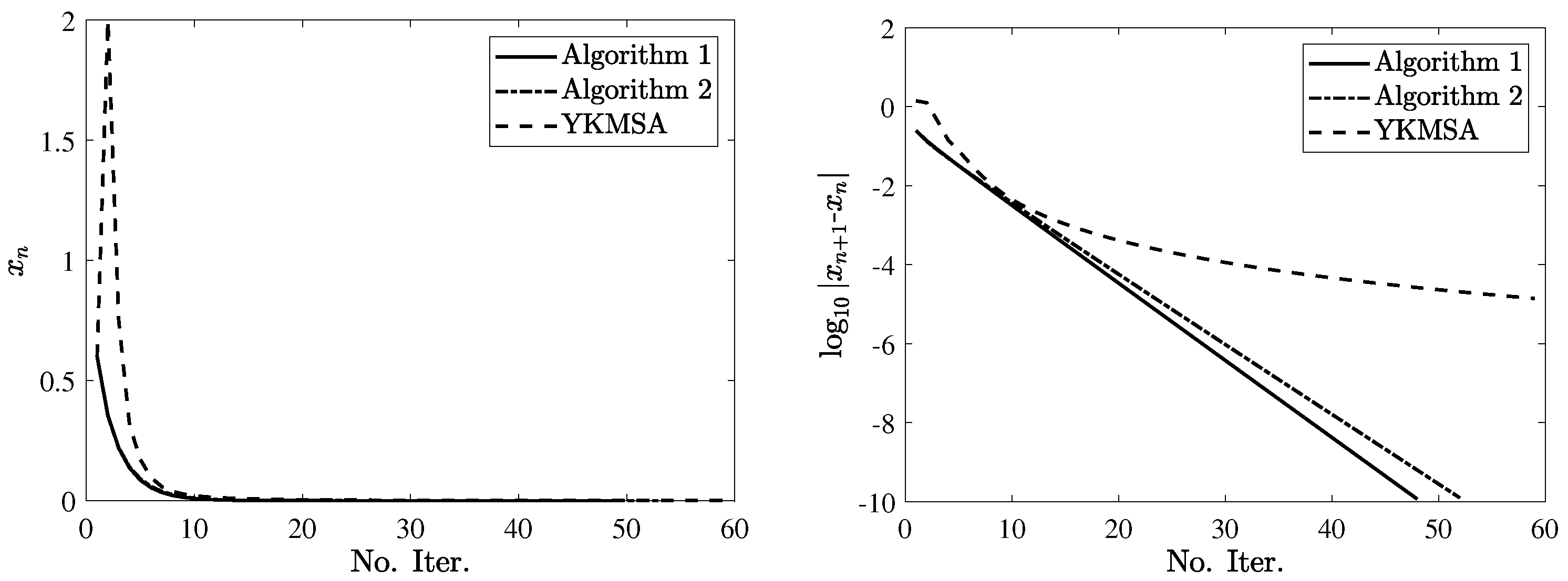
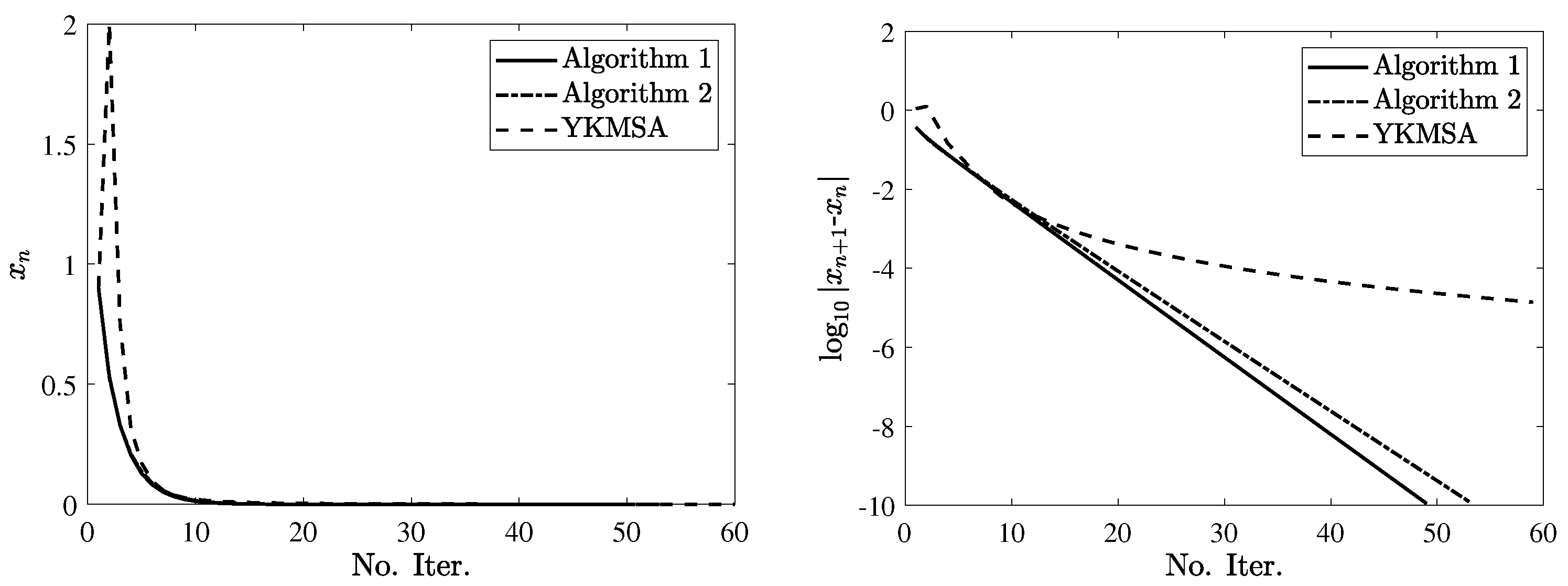
Example 6.

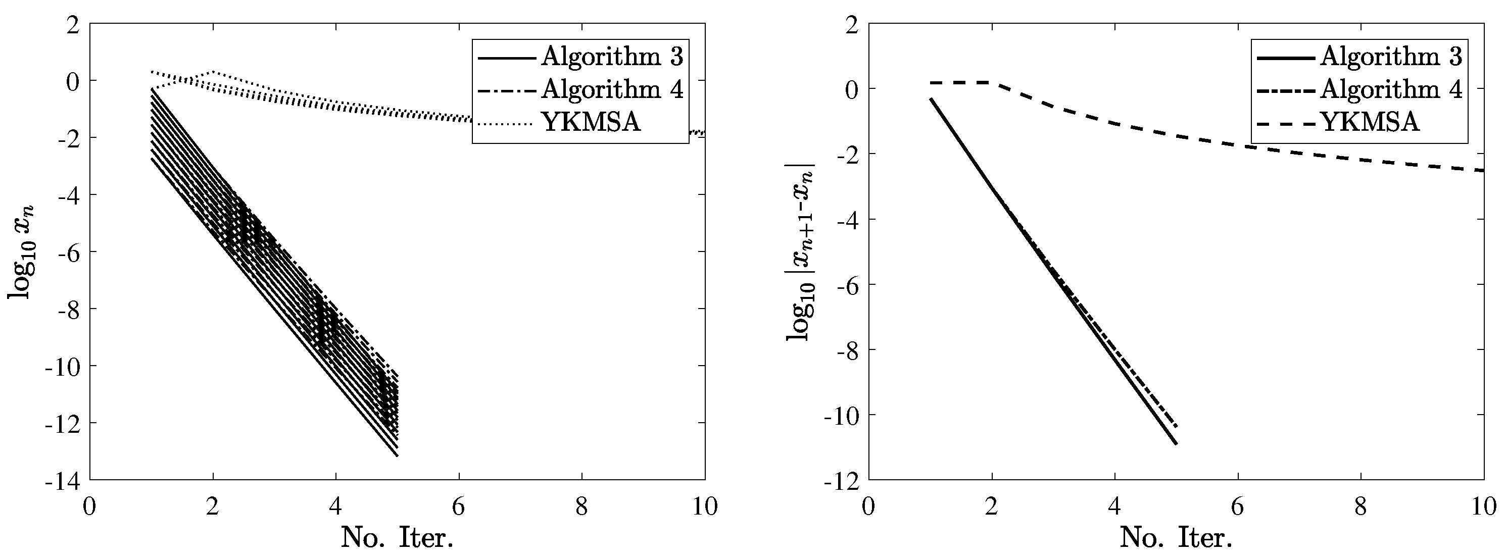
Let $\mathcal{H}=\mathbb{R}$. Let $S\left(x\right):=x/2$, and T be defined by (13) with $r=3/4$. It is not difficult to verify that $\left\{0\right\}$ is the only common solution of (4). Note that S and T satisfy all conditions in Theorem 1 and Corollary 1; thus, the sequences generated by Algorithms 1 and 2 converge to 0 together.

Example 7.

Let $\mathcal{H}=\mathbb{R}$. Let $i\in \{1,2,\cdots ,10\}$, $S_i\left(x\right):=(0.5-0.02i)x$, and $T_i$ be defined by (13) with $r_i=0.6-0.02i$. The common solution of (3) is $\left\{0\right\}$. It is easy to see that $S_i$ and $T_i$ satisfy all conditions in Theorem 2 and Corollary 2, which leads that the sequences produced by Algorithms 3 and 4 converge to 0.

We compare the convergence speed of Algorithms 1–4 to YKMSA [14] (i.e., (8)) through Examples 6 and 7. The parameters are set as follows. In the proposed algorithms, set ${\alpha }_n=1/(9n+1)$, ${\beta }_n=1/4$, ${\gamma }_n=n/(9n+9)$, ${\delta }_n=0.99-1/(4n+1),{\eta }_n=1/n$, and let ${\alpha }_n^{\left(i\right)}={\alpha }_n,{\beta }_n^{\left(i\right)}={\beta }_n,{\gamma }_n^{\left(i\right)}={\gamma }_n,{\delta }_n^{\left(i\right)}={\delta }_n,{\eta }_n^{\left(i\right)}={\eta }_n$. For YKMSA, set $a_n=b_n=(n^2-1)/\left(2n^2\right)$, $c_n=1/n^2$, $u_n=1+1/n$ according to Lemma 3.1 [14]. The stop criterion is set as $\parallel x_{n+1}-x_n\parallel \le {10}^{-10}$ or a maximum iteration of ${10}^3$. Take the initial points as $0.6$ and $0.9$ for Example 6 and $0.5$ for Example 7. The numerical results are shown in Figure 1, Figure 2 and Figure 3. As shown in the figures, it can be observed that both the one-step and multistep algorithms involving implicit rules perform slightly better than explicit algorithms. Furthermore, as the one-step and multistep YKMSAs [14] contain Halpern-type constants, the proposed algorithms in this article converge much faster than YKMSA.

According to (2), we have shown that GCSVIOE is equivalent to a CSOS. Now, we give the following multistep implicit Algorithm 5 and Theorem 3 to find the solution of GCSVIOE.

Algorithm 5 Multistep implicit iteration for GCSVIOE

Choose an initial point $x_1\in \mathcal{H}$, and for any $n\in \mathbb{N}$ do the following: $$\left\{\begin{array}{l}{z}_n^{\left(1\right)}={\eta }_n^{\left(1\right)}{z}_n+(1-{\eta }_n^{\left(1\right)})x_n^{\left(1\right)},\\ y_n^{\left(1\right)}={\delta }_n^{\left(1\right)}{z}_n^{\left(1\right)}+(1-{\delta }_n^{\left(1\right)})P_{Q_1}(z_n^{\left(1\right)}-r{F}_1{z}_n^{\left(1\right)}),\hfill \\ x_n^{\left(1\right)}=(1-{\alpha }_n^{\left(1\right)}-{\beta }_n^{\left(1\right)}-{\gamma }_n^{\left(1\right)})S_1\left(x_n\right)+{\beta }_n^{\left(1\right)}{x}_n+{\gamma }_n^{\left(1\right)}{y}_n^{\left(1\right)},\hfill \\ \mathrm{for}i=2,3,\cdots ,p,\\ z_n^{\left(i\right)}={\eta }_n^{\left(i\right)}{z}_n^{(i-1)}+(1-{\eta }_n^{\left(i\right)})x_n^{\left(i\right)},\hfill \\ y_n^{\left(i\right)}={\delta }_n^{\left(i\right)}{z}_n^{\left(i\right)}+(1-{\delta }_n^{\left(i\right)})P_{Q_i}(z_n^{\left(i\right)}-r{F}_i{z}_n^{\left(i\right)}),\hfill \\ x_n^{\left(i\right)}=(1-{\alpha }_n^{\left(i\right)}-{\beta }_n^{\left(i\right)}-{\gamma }_n^{\left(i\right)})S_i\left(x_n^{(i-1)}\right)+{\beta }_n^{\left(i\right)}{x}_n^{(i-1)}+{\gamma }_n^{\left(i\right)}{y}_n^{\left(i\right)},\hfill \\ x_{n+1}=x_n^{\left(p\right)}.\hfill \end{array}\right.$$ The real sequence $\left\{{\alpha }_n^{\left(i\right)}\right\},\left\{{\beta }_n^{\left(i\right)}\right\},\left\{{\gamma }_n^{\left(i\right)}\right\},\left\{{\delta }_n^{\left(i\right)}\right\}$, and $\left\{{\eta }_n^{\left(i\right)}\right\}$ satisfies the following conditions: (i) ${\alpha }_n^{\left(i\right)},{\beta }_n^{\left(i\right)},{\gamma }_n^{\left(i\right)},{\delta }_n^{\left(i\right)},{\eta }_n^{\left(i\right)}$ are all in $[0,1]$; (ii) $\frac{{\alpha }_n^{\left(i\right)}+{\gamma }_n^{\left(i\right)}}{1-{\alpha }_n^{\left(i\right)}-{\beta }_n^{\left(i\right)}-{\gamma }_n^{\left(i\right)}}\le 1-c_i$; (iii) $\frac{{\alpha }_n^{\left(i\right)}}{{\gamma }_n^{\left(i\right)}}\to 0$, ${\eta }_n^{\left(i\right)}\to 1$, and ${\sum }_{j=1}^{\infty }{\alpha }_j^{\left(i\right)}=\infty$; (iv) ${ϵ}_i\le {\delta }_n^{\left(i\right)}\le 1-{ϵ}_i$; here, ${ϵ}_i>0$ is a positive constant; (v) $r\in (0,\underset{i\in 1,2,\cdots ,p}{min}2{\sigma }_i/{\mu }_i^2)$.

Theorem 3.

For all $i\in \{1,2,\cdots ,p\}$, suppose that $S_i:\mathcal{H}\to \mathcal{H}$ is a $c_i$—contraction operator and $F_i:Q_i\to \mathcal{H}$ is a ${\sigma }_i/{\mu }_i^2$-inverse strongly monotone operator, where $Q_i$ is a nonempty closed convex subset of $\mathcal{H}$. Then, the sequence $\left\{x_n\right\}$ generated by Algorithm 5converges strongly to the solution of (2), that is,GCSVIOEis solved by Algorithm 5.

Proof. 

For any $i\in \{1,2,\cdots ,p\}$, let $T_i:=P_{Q_i}(I-r{F}_i)$. Then, according to [26], one has $T_i$, which is a nonexpansive operator for all $i\in \{1,2,\cdots ,p\}$. Thus, for each $i\in \{1,2,\cdots ,p\}$, $T_i$ is also 1-Lipschitzian-continuous and $(1,0)$-asymptotically demicontractive, and $I-T_i$ is demiclosed at 0 [27]. Recall Example 5; one can easily see that $T_i$ is also uniformly asymptotically regular for all $i\in \{1,2,\cdots ,p\}$. Hence, $T_i$$(i=1,2,\cdots ,p)$ satisfies all the conditions required in Theorem 2.

Then, by directly applying Theorem 2, one sees that the sequence $\left\{x_n\right\}$ generated by Algorithm 5 converges strongly to a point in ${\bigcap }_{i\in \{1,2,\cdots ,p\}}Fix\left(S_i\right)\cap Fix\left(T_i\right)$. This completes the proof. □

5. Conclusions

In this paper, to answer Question 1, we propose a brand-new multistep algorithm (i.e., Algorithm 3) for solving CSOSs (3), which are highly related to nonlinear optimization problems. We first give two strong convergence theorems for both one-step and multistep iterations, utilizing the implicit rule for CSOSs that involve asymptotically demicontractive operators. In order to show the efficiency of the proposed algorithms, two numerical simulations on single-set and multi-set CSOSs are given in Section 4 and are also applied to GCSVIOE.

However, the following two areas are worthy of future research:

(i)

The common solution of two finite or infinite asymptotically demicontractive operators requires in-depth exploration.

(ii)

Convergence for CSOSs involving multivalued operators—see [28].