Robust μ-Controller for Automatic Glucose Regulation for Type I Diabetes Mellitus

Abstract

Type I diabetes mellitus is a serious autoimmune condition impacting a large population around the world that need a daily infusion of insulin substitutes to regulate blood glucose levels within healthy limits. The purpose of the study was to design a robust $\mu$-controller based on an uncertain linear-time invariant (LTI) representation of the Hovorka model for glucose–insulin metabolism. The model set was obtained using linearization around an equilibrium point and adding parametric uncertainty to account for the time delay variation between plasma glucose concentration and its subcutaneous measurement. As a result, the robust stability and performance of the closed loop were proved using the structured singular value $\mu$. The performance of the designed controller was also checked with a numerical simulation in connection with the nonlinear model.

1. Introduction

Glucose has a primary place in energy metabolism as an initial substrate for glycolysis. Glycolysis in conjunction with the Krebs cycle is the basic catabolic pathway, producing nicotinamide adenine dinucleotide (NADH). NADH is used in processes of oxidative phosphorylation, which generates adenosine triphosphate (ATP)—the main energy source required for cell biochemical reactions. On the other hand, glucose is a major precursor for the synthesis of different carbohydrates such as glycogen, glycolipids, glycoproteins, and proteoglycans [1]. The transport of glucose across cell membranes is facilitated by a large group of receptors called glucose transporters (GLUTs). Some GLUT receptors are unidirectional and concentration-dependent—such as GLUT3 expressed in neuron cells. Bidirectional GLUT3 receptors are expressed in liver cells and pancreatic beta cells. Skeletal and cardiac muscle cells, as well as adipose tissue cells, express the insulin regulated GLUT4 receptor. Maintaining glucose homeostasis is an essential feature of adaptation for all mammals, and it is a critical requirement for normal body function and organism survival. Homeostatic mechanisms are mediated by various hormones and neuropeptides, released by the brain, pancreas, liver, intestine, etc. The most important regulators are the hormone insulin and its antagonist glucagon, both of which are secreted from the pancreatic beta cells, located in the so-called Langerhans islets.

Type 1 diabetes is a chronic autoimmune disease, characterized by the T-cell-mediated destruction of insulin-producing $\beta$ cells in pancreatic islets, that results in insulin deficiency [2,3]. Subjects with type 1 diabetes lack the ability for natural insulin secretion and need an intake of synthetic insulin replacement therapy administered subcutaneously or, in case of emergency, intravenously. Serious life-treating complications of type 1 diabetes associated with hyperglycemia are diabetic ketoacidosis, hyperosmolar hyperglycemic state, etc. On the other hand, a hypoglycemic period can also be dangerous, leading to unconsciousness, seizures, and others. Late complication of type 1 diabetes associated with poor control of blood glucose levels is categorized as microvascular (retinopathy, nephropathy, and neuropathy) and macrovascular (cardiovascular disease, cerebrovascular disease, and peripheral vascular disease).

The concept of an artificial pancreas (AP) system has been investigated for several decades, with many successful experiments in clinical trials or in field applications. The development of AP systems started with intravenous administration prototypes, which give fast and robust response [4]. The invasive nature of intravenous intervention limited the practical application of such systems in the past. With the appearance of subcutaneous glucose-monitoring sensors [5] and insulin-delivery pumps [6], the potential for the development of a wearable extracorporal AP system is increased. However, the subcutaneous sensing and delivery path introduce additional absorption delay in the control system, which fundamentally limits the achievable regulation performance [7]. The main problem with the subcutaneous AP system is that insulin already administered cannot be removed, which can easily cause under-regulation after meals and, hence, hypoglycemic periods. A critical in measure to reduce such effects is to use next-generation short-acting insulin [8]. Some AP systems benefit from dual hormone control algorithms using glucagon to counteract insulin with a structure from three controllers for basal delivery, aggressive insulin and glucagon controller to prevent hypoglycemia [9]. An alternative approach to CGM can be found in [10], proposing an integrated islet-based biosensor to mimic the inborn regulation capabilities.

The AP system is obviously within the framework of feedback control theory and poses an interesting challenge where various methods can be effectively applied. There are a couple of notable practical applications for AP systems, an open source project OpenAPS [11], Medtronic MiniMed [12], Nightscout [13], and intelligent control assistant for diabetes (INCA) [14]. Authors in [15] clinically evaluate a system that integrates a control algorithm with standard subcutaneous sensors and pumps with the implementation of an adaptive PD controller. However, introduction of novel algorithms for glucose regulation in medical trial is approached with caution; for example,  Ref. [16] gives an extensive review of the possible hazards associated with the closed-loop AP system with respect to physiological changes in the patient. An established benchmark for testing a developed control system is the UVa/Padova large-scale simulator [17] for type 1 diabetes treatment. The American Food and Drug Administration (FDA) has established that Padova simulator results can be used as a substitute for pre-clinical animal model studies.

Since the primary exogenous disturbance in the AP system is the meal intake, from a control perspective, it would be most beneficial to assume that the treated subject is announcing their meals around 15 min in advance by specifying the equivalent amount of carbohydrate units for the meal. In response, the AP system would calculate the appropriate dose of bolus to be administered. The meal announcement could be prone to errors in practical applications and requires considerable discipline from the subject. There have been many attempts to design an AP system for unannounced meals. For example, Ref. [18] used a fifth-order switched glucose model to build an extended meal disturbance observer. The resultant control system shows good performance in the A and B zones in the control variability grid analysis (CVGA) plot. Insulin delivery is a continuous working system that must be robust to model uncertainty or intersubject variability. Also, Ref. [19] developed a meal-detection algorithm applying an unscented Kalman filter to a Bergman glucose model which successfully detects meals and snacks to administrate the boluses in case of unannounced meals and prevent hyperglycemia. Ref. [20] propose a closed-loop design that operates in a fully automated fashion, without requiring manual meal announcements. Authors in [21] attempted a novel approach using reinforcement learning techniques based on a temporal cost function with discount factors reflecting the individual’s specific pharmacological characteristic. The aim of the algorithm is to handle unannounced meal intake, which was investigated in Padova simulations. In [22], a novel event-triggered modification of model predictive techniques was applied, which ensures glucose regulation within safe limits. Control approaches extending the conventional PID controllers are also possible; for example, Ref. [23] implemented multiple-model PID control tuned with a genetic optimization algorithm. The weighting between multiple controllers was decided with a fuzzy gain scheduling strategy. An additional onboard insulin constraint and pump stopping are described as safety mechanisms. Insulin activity can vary depending on time of day, other health conditions, and physical exercise. The topic of model-based anomaly detection in AP systems based on machine learning is also present in research [24]. The common logic for designing AP systems in the presence of long delays is to estimate blood glucose and blood insulin concentrations from the subcutaneous measurements and also to predict the future insulin activity and insulin on board. There are successful studies with zone model predictive control [25]. The response of the subcutaneous glucose sensor is typically modeled as a first-order transfer function, with the impact of absorption lag on sensor precision [26]. The lag from subcutaneous insulin administration is approximately 90 min–50 min for insulin absorption, 30 min for insulin action, and 10 min for glucose measurement [27]. One approach to modeling the dynamic of such a lagged process is through delayed differential equations [28].

There are some important results in the literature concerning the robust control of AP systems. Reference [29] is similar to the present work through its use of the $\mu$-synthesis technique, assuming bounded variation in several meaningful physiological parameters. The controller design was carried out on the basis of the Sorensen pharmacokinetic model, assuming relatively large uncertainty bounds in four parameters. The results of this paper provide a promising indication that the $\mu$-controller is an appropriate approach for calculation of the insulin infusion rate. The difference with the present work is that we use a new uncertainty model where we take into account the variability of the glucose measurement dynamics. The authors of [30,31] use the model from the first version of the UVa/Padova simulator, which is of the 13th order with respect to insulin infusion. The controller design is achieved through closed-loop $H_{\infty }$ norm minimization. It is well known that such an approach does not guarantee the robust performance of the closed loop by design and may require the optimization problem to be solved multiple times to obtain robustness. In [32], a multi-objective $H_2/H_{\infty }$ design is employed. The solution to the optimization problem is obtained with the help of linear matrix inequality (LMI) methods. The obtained results are acceptable. However, in contrast to the model utilized in the present paper, the authors there use a low-order Bergman model.

The purpose of the present research was to characterize uncertainty of one of the commonly employed pharmacokinetic models with a bounded model set that accounts simultaneously for the sensor lag and the intersubject variability. Then, using the recent results from robust control theory, we designed a state feedback controller minimizing the structured singular value $\mu$ of the closed-loop system to achieve robust stability and robust performance. The resultant controller is from the 24th dynamic order. Its performance is verified for the adult population from the UVa/Padova simulator. Because the obtained controller is of a relatively high order, based on its Hankel singular values, we reduced its order to 10th. The reduced-order controller still preserves the robust performance of the closed-loop system, even when tested with a nonlinear model simulator from UVa/Padova.

Section 2 presents briefly the nonlinear Hovorka model, Section 3 extends it with an uncertain element in order to convert it into a model-set, Section 4 details the synthesis of the $\mu$-controller using mixed-sensitivity weighting, and Section 5 presents the results from simulation with the Hovorka model and with the UVa/Padova simulator.

2. Nonlinear Glucose Metabolism Model

Since the $\mu$-control design is a model-based procedure, we start with a mathematical formulation of glucose–insulin dynamics. There are various models employed in the field of AP system analysis and design—Hovorka [33], Bergman [34], etc. A key challenge is model parameter estimation, which can be approached using the methods of system identification theory; for example, Ref. [35] employs weighted recursive least squares to estimate an individual model of the treated subject with guaranteed stability. The Hovorka model was developed as a predictive model for subjects with type 1 diabetes with prescribed insulin replacement therapy with a short-term acting Lispro. It characterizes glucose-insulin dynamics as a two-compartment pharmacokinetic model incorporating gut absorption dynamics obtained from the intake of carbohydrates, subcutaneous insulin absorption dynamics, insulin interaction with the plasma glucose, and rate of endogenous glucose production. The two compartments in the model are the subcutaneous fluid and the plasma. Furthermore, the model specifies the kinetic rates of species transfer between the compartments.

Here, we translated one version of the Hovorka model into a system of state space equations in Cauchy form. The state vector of the model is described in

Table 1. Model state variables.

Variable	Symbol	Unit
Gut CHO	$x_1$	mmol
Plasma CHO	$x_2$	mmol/L
Subcutaneous insulin	$x_3$	IUs
Plasma insulin	$x_4$	IUs/L
Plasma glucose	$x_5$	mmol/L
ECF glucose	$x_6$	mmol/L
IA on glucose distribution	$x_7$	L/min
IA on glucose disposal	$x_8$	L/min
EGP rate	$x_9$	mmol/min

CHO—carbohydrate concentration, ECF—extracellular fluid, EGP—endogenous glucose production, IA—insulin action.

. The second-order gut absorption dynamics with states $x_1$ and $x_2$ is

$$\begin{array}{c}{\dot{x}}_1=-{\tau }_D^{-1}{x}_1+K_{AG}{M}_{G}d\left(t\right)\hfill \\ {\dot{x}}_2=-k_g{x}_2+\left({\tau }_D^{-1}{V}_G\right)x_1\hfill \end{array},$$

(1)

with $d\left(t\right)$ being carbohydrate (CHO) intake rate in g/min per kg of body weight. From the control perspective, $d\left(t\right)$ represents an exogenous disturbance variable. It depends on meal intake even though it can be assumed to a certain extent based on the subject meal announcement. Otherwise, it can be regarded as a stochastic signal with impulse-like nature. The subcutaneous insulin infusion is also a second-order model with states $x_3$ and $x_4$

$$\begin{array}{c}{\dot{x}}_3=-{\tau }_S^{-1}{x}_3+u\left(t\right)\hfill \\ {\dot{x}}_4=-k_e{x}_4+{\left({\tau }_S{V}_I\right)}^{-1}{x}_3\hfill \end{array},$$

(2)

where $u\left(t\right)$ represents the insulin replacement infusion rate in insulin units (IUs) per minute. The signal $u\left(t\right)$ is the manipulated variable in the system, and it is calculated by the controller. Conventional AP controllers, which are heuristically tuned, assume that the control signal is composed of basal and bolus components to mimic the physiological manner of insulin regulation. However, we assume basal infusion, since that will not make a difference from mathematical perspective for the $\mu$-controller design.

The nonlinear part of the model concerns the interaction between glucose and insulin. The glucose concentration is presented in the extracellular fluid as a state $x_6$ and in the plasma as a state $x_5$

$$\begin{array}{c}{\dot{x}}_5=k_g{x}_2-F_{01,c}-x_5{x}_7+k_{12}{x}_6+S_{EGP}\left(t\right)\hfill \\ {\dot{x}}_6=x_5{x}_7-k_{12}{x}_6-x_6{x}_8\hfill \end{array}.$$

(3)

The nonlinearity in this model, as in many metabolic models, arises from the multiplicative terms correlating amplitudes of 2 states—in this case, $x_5{x}_8$ and $x_6{x}_9$. This reflects a pharmacokinetic law that the reaction rate between 2 species is proportional to their concentration. The term $F_{01,c}=F_{01}{x}_5/(1+x_5)$ represents glucose elimination due to glycolysis. From a control theory perspective, this is a smooth nonlinearity and can be well approximated with first-order Taylor expansion for a fixed regulation point. The term

$$S_{EGP}\left(t\right)=S_{EGP,0}(1-(tanh\left(2.6518(x_9\left(t\right)-0.5)\right)+1)/2),$$

(4)

represents the endogenous glucose production (EGP) rate, and its form is slightly modified from the original Hovorka model, where it has a point with a discontinuous derivative. Hence, we approximated the nonlinearity with the help of the tanh function, which is differentiable.

The final component in the model describes the insulin activity with states $x_7$, $x_8$, and $x_9$ for disposition, disposal, and EGP, respectively, as

$$\begin{array}{c}{\dot{x}}_7=-k_{a,1}{x}_7+k_{b,1}{x}_4\hfill \\ {\dot{x}}_8=-k_{a,2}{x}_8+k_{b,2}{x}_4\hfill \\ {\dot{x}}_9=-k_{a,3}{x}_9+k_{b,3}{x}_4,\hfill \end{array}$$

(5)

The numerical values of the model parameters assumed for an average adult subject, together with their physical units are summarized in

Table 2. Model parameters.

Parameter	Symbol	Unit	Value
Transfer rate	$k_{12}$	L/min	0.066
Deactivation rate	$k_{a,1}$	L/min	0.006
Deactivation rate	$k_{a,2}$	L/min	0.06
Deactivation rate	$k_{a,3}$	L/min	0.03
Insulin transport sensitivity	$S_{I,1}$	L/U	5.12
Insulin disposal sensitivity	$S_{I,2}$	L/U	0.82
Insulin EGP sensitivity	$S_{I,3}$	L/U	52.0
CHO metabolic rate	$k_e$	L/min	0.033
CHO absorption timeconstant	${\tau }_D$	min	30.0
Insulin absorption timeconstant	${\tau }_S$	min	60.0
CHO utilization	$K_{AG}$	-	0.8
Glucose equivalent per unit CHO	$M_G$	mmol/g	6.94
Glucose distrib. volume	$V_G$	L	11.2
Insulin distrib. volume	$V_I$	L	8.4
Glucose consumption	$F_{0,1}$	mmol/min	0.679
Liver glucose production	$S_{EGP,0}$	mmol/min	1.127

. The numerical values of these parameters may exhibit intersubject variability or even interday variability for a single subject. Estimation of these parameters and their deviations is an interesting problem and certainly influences the robustness of the AP system. But a researcher may easily be misguided by considering independent uncertainty variations in all these parameters at the same time. The sensitivity of the glucose concentration to any of them has to be examined concerning the internal feedback loops in the model and with respect to the external insulin infusion rate controller, since this feedback will reduce sensitivity of the closed-loop system to uncertainty variations. Finally, in many cases, parametric variations in a model can be represented as an equivalent signal disturbance acting on the output or input of the system.

3. Uncertain LTI Model

The nonlinearity in the Hovorka model from the previous section is concentrated in the equations for plasma and subcutaneous glucose concentrations. The rest of the model equations are linear. The design of the $\mu$-controller requires an uncertain LTI representation of the system. We convert the Hovorka model to such representation using two steps. First, we linearize the model using analytic Taylor approximation around the operating point. And second, we introduce an additional equation to the model reflecting the major difficulty in the AP systems, i.e., the delay between plasma glucose concentration and its subcutaneous measurement. The linearization is performed for an operating point with the following coordinates

$$x_0={(4.2,4.2,0.173,0.173,10.2,10.2,645,6450,16.1)}^T$$

(6)

and the resultant linearized model is in the following matrix-vector form

$$\begin{array}{c}\dot{\overrightarrow{x}}\left(t\right)=A\overrightarrow{x}\left(t\right)+Bu\left(t\right)+Gd\left(t\right)\hfill \\ y\left(t\right)=C\overrightarrow{x}\left(t\right)\hfill \end{array}$$

(7)

where the matrices $A\in {\mathbb{R}}^{9x9}$, $B\in {\mathbb{R}}^{9x1}$, $C\in {\mathbb{R}}^{1x9}$, and $G\in {\mathbb{R}}^{9x1}$ are of suitable dimensions.

To account for the uncertain time delay in the system, we assume a single uncertain parameter $T_{unc}\in [10,100]$ with a nominal value of $T_{unc}=50$ min. Therefore, the linearized model is extended with one additional equation

$${\dot{x}}_{unc}\left(t\right)=-\frac{1}{T_{unc}}{x}_{unc}\left(t\right)+\frac{1}{T_{unc}}{x}_5\left(t\right).$$

(8)

This essentially extends the dynamic model between plasma and ECF glucose concentration. The uncertainty of this parameter transforms the linearized model into a model set $\mathcal{M}$, accounting for all possible values in the $T_{unc}$ range. Then, we can extend model (3) with the state $x_{unc}$

$$\left(\begin{array}{c}\dot{x}\left(t\right)\\ {\dot{x}}_{unc}\left(t\right)\end{array}\right)=\left(\begin{array}{cc}A& 0\\ T_{unc}^{-1}C& T_{unc}^{-1}\end{array}\right)\left(\begin{array}{c}x\left(t\right)\\ x_{unc}\left(t\right)\end{array}\right)+\left(\begin{array}{c}B\\ 0\end{array}\right)u.$$

(9)

The disturbance signal d, that represents the carbohydrate intake rate, is dropped from the model at this stage. The reasons for this are as follows. The equivalent effect of the disturbance d over the BG concentration y can be represented with a transfer function $T_{yd}\left(s\right)$, extracted from the linearized model, such that $y\left(s\right)=T_{yu}\left(s\right)u\left(s\right)+T_{yd}\left(s\right)d\left(s\right)$. As can be seen, the signal $d\left(t\right)$ can be thought of as output (loading) disturbance over the closed-loop system, weighted by the transfer function $T_{yd}\left(s\right)$. The actual response of the closed-loop AP system to this disturbance will be determined by the output sensitivity function of the loop $S_o={(I+T_{yu}K)}^{-1}$, which depends only on the open loop transfer function $T_{yu}$ and on the controller K but not on the weighting filter $T_{yd}$. In addition, from fundamental closed-loop relations, minimization of the effect of loading disturbance is equivalent to a reduction in the tracking error of the system $e=r-y$ between the target BG concentration r and the measured one y. The role of the weighting filter $T_{yd}$ is then only to impose some band limiting action over the frequency spectrum of the meal intake disturbance. Due to the intersubject variability, the $T_{yu}$ in practice will incorporate additional uncertain elements; however, the inclusion of such additional uncertainty is not expected to significantly affect the overall closed-loop performance.

After the extension of the model with the uncertain element $x_{unc}$, the resultant output signal will be produced as

$$y\left(t\right)=x_{unc}\left(t\right).$$

(10)

The model set $\mathcal{M}$ can be examined in the time and frequency domain by conducting random sampling over the range of uncertain parameter $T_{unc}$ to obtain a set of representative LTI systems. The random sampling approach does not guarantee that minimal and maximal deviations of the characteristics will be captured, but since such extremes will depend on more complicated analytical examination, the random sampling approach is usually enough for practical applications. Since the linearized model (3) is valid only for a deviations from the operating point where BG levels are regulated, it can be conveniently examined in frequency domain using the Bode diagram in Figure 1.

As can be seen, the effect of the uncertain parameter is evident in both magnitude and phase responses of the uncertain LTI model. Since the parameter $T_{unc}$ has a physical significance as a time-constant, we observe its impact as a shift in the bandwidth of the open-loop system, determined by the cut-off frequency. The impact of the uncertainty on the magnitude response increases with the frequency, which, however, does not impose any constraints on the achievable performance of the closed loop in the low-frequency range. The impact of the uncertainty in the phase response is more pronounced and extends around the cut-off frequency up to the low-frequency domain. The critical zone for system stability and performance is the phase angle of $-{180}^{\circ }$, where it can be seen that phase response uncertainty is accumulated. As long the phase response is associated with the delay of the open-loop reaction to an applied input action, such uncertain delay can be again related to the difficulties encountered in the conventional AP systems based on subcutaneous CGM—even if the system is tuned to one subject, its response will not be guaranteed across a larger group of individuals.

4. Mixed-Sensitivity $\mathbf{\mu }$-Controller Design

It was established that the main benefit of the feedback loop is that uncertainty of the closed-loop system can be made smaller than the uncertainty of the open loop system. A large variety of methods exist that properly capture the features of the underlying plant uncertainty, and a controller has been proposed which can minimize the uncertainty effect on the system performance. $\mu$-synthesis is a powerful procedure that explicitly accounts for the uncertain model parameters. The purpose of structured singular value $\mu$ is to characterize the stability range of the $M-\mathrm{\Delta }$ configuration

$${\mu }_{\mathrm{\Delta }}\left(j\omega \right)=\frac{1}{min\{\overline{\sigma }\left(\mathrm{\Delta }\right):\parallel \mathrm{\Delta }{\parallel }_{\infty }<1,det(I-M\left(j\omega \right)\mathrm{\Delta })=0\}}.$$

(11)

$M\left(j\omega \right)$ represents a deterministic LTI system connected in a feedback configuration with a static matrix $\mathrm{\Delta }$ containing block diagonal uncertain elements. In other words, for each frequency $\omega$, $\mu \left(j\omega \right)$ is calculated as an inverse of the maximal singular value of the uncertain block matrix $\mathrm{\Delta }$, which can drive the $M-\mathrm{\Delta }$ feedback loop at the stability bounds. If the system possesses robust stability for a given frequency, then the value of $\mu <1$ for this frequency because for all admissible values of the uncertain element $\mathrm{\Delta }$ with infinity norm smaller than the unit, the closed-loop configuration will have no poles with a real positive part, i.e., will remain stable. In addition, the proximity of the $\mu$ value to the unit bound will characterize the margin of robustness, or how much the uncertainty can be increased while the system preserves stability. The structured singular value can be used also to characterize system performance by reformulating performance requirements into stability ones.

The purpose of the $\mu$ design is to select the controller K such that the closed loop will keep its stability and performance for all uncertainties ${\parallel \mathrm{\Delta }\parallel }_{\infty }<1$. With the help of lower fractional transform (LFT) ${\mathcal{F}}_l$, which represents the closed-loop interconnection between the controller and the open-loop system, the design problem is expressed as

$$\underset{K}{min}{\parallel {\mu }_{\mathrm{\Delta }}\left({\mathcal{F}}_l(M,K)\right)\parallel }_{\infty }.$$

(12)

We sought an LTI controller K to minimize the peak value of the structured singular value $\mu$, hence maximizing the robust stability margins of the system with respect to the prescribed uncertainty bounds in the model.

4.1. Model Transformations

For the described uncertain LTI model of the AP system, we have a single scalar uncertain element $\mathrm{\Delta }\in [-1,1]$, corresponding to the time constant $T_{unc}$. To show this, we exploit the structure of the uncertain model (3) and convert it into the framework of robust control theory [36,37], i.e., obtaining its $M-\mathrm{\Delta }$ representation. The goal in $M-\mathrm{\Delta }$ structure is to decompose the system into deterministic and uncertain subsystems, such that all fixed parameters are in a dynamic M subsystem, and all uncertain parameters are in a static $\mathrm{\Delta }$ block. First, let the uncertain term admit a representation

$$T_{unc}^{-1}={\overline{T}}_{unc}^{-1}+\delta ,$$

(13)

where ${\overline{T}}_{unc}^{-1}$ is equal to the central value in the range of the uncertain element $T_{unc}^{-1}$, and the deviation $\delta \in [{\delta }_{min},{\delta }_{max}]$ is calculated such that the range of $T_{unc}^{-1}$ matches the range of $T_{unc}\in [10,100]$. Therefore,

$$\begin{array}{c}\hfill {\overline{T}}_{unc}^{-1}=(min\left(T_{unc}^{-1}\right)+max\left(T_{unc}^{-1}\right))/2=0.055,\end{array}$$

(14)

$$\begin{array}{c}\hfill {\delta }_{min}=min\left(T_{unc}^{-1}\right)-{\overline{T}}_{unc}^{-1}=-0.045,\end{array}$$

(15)

$$\begin{array}{c}\hfill {\delta }_{max}=max\left(T_{unc}^{-1}\right)-{\overline{T}}_{unc}^{-1}=0.045.\end{array}$$

(16)

The result of this representation is that we can additively separate the uncertain term from the model Equations (3) such as

$$\left(\begin{array}{c}\dot{x}\\ {\dot{x}}_{unc}\end{array}\right)=\left(\begin{array}{cc}A& 0\\ {\overline{T}}_{unc}^{-1}C& {\overline{T}}_{unc}^{-1}\end{array}\right)\left(\begin{array}{c}x\\ x_{unc}\end{array}\right)+\left(\begin{array}{cc}0& 0\\ C\delta & \delta \end{array}\right)\left(\begin{array}{c}x\\ x_{unc}\end{array}\right)+\left(\begin{array}{c}B\\ 0\end{array}\right)u.$$

(17)

Therefore, we can replace the term containing the uncertain element $\delta$ with a new external signal $y_{\mathrm{\Delta }}=\mathrm{\Delta }{u}_{\delta }$, where $\left|\mathrm{\Delta }\right|\le 1$ is a static gain matrix (with dimension 1 in our case), accumulating the uncertainty of the system. Therefore, the $M-\mathrm{\Delta }$ representation becomes

$$\begin{array}{c}\hfill \left(\begin{array}{c}\dot{x}\\ {\dot{x}}_{unc}\end{array}\right)=\left(\begin{array}{cc}A& 0\\ {\overline{T}}_{unc}^{-1}C& {\overline{T}}_{unc}^{-1}\end{array}\right)\left(\begin{array}{c}x\\ x_{unc}\end{array}\right)+\left(\begin{array}{cc}0& B\\ 1& 0\end{array}\right)\left(\begin{array}{c}{y}_{\mathrm{\Delta }}\\ u\end{array}\right),\end{array}$$

(18)

$$\begin{array}{c}\hfill \left(\begin{array}{c}{u}_{\mathrm{\Delta }}\\ y\end{array}\right)=\left(\begin{array}{cc}{k}_{\delta }C& k_{\delta }\\ 0& 1\end{array}\right)\left(\begin{array}{c}x\\ x_{unc}\end{array}\right),\end{array}$$

(19)

where $k_{\delta }={\delta }_{min}^{-1}={\delta }_{max}^{-1}$ is a scaling constant to map the range of parameter $\delta$ into the range $[-1,1]$ (Figure 2). As can be seen, the resultant dynamic model does not contain any uncertain elements. The uncertainty is represented as an external $\mathrm{\Delta }$ element interacting with the model as a feedback generator of disturbances $y_{\mathrm{\Delta }}$. The participation of the uncertain parameters in a feedback loop is a critical factor impacting the internal stability of the modeled system, which in the case of AP can be interpreted in the line that there exists some uncertainty in the organism which can determine the stability of the BG concentration.

For further analysis, we need the frequency domain representation of the above relations, which can be obtained by taking the Laplace transform of both sides of the equation and applying matrix inversion and multiplication formulas for block matrices to obtain

$$\left(\begin{array}{c}{u}_{\mathrm{\Delta }}\\ y\end{array}\right)=\frac{1}{s-{\overline{T}}_{unc}^{-1}}\left(\begin{array}{cc}{k}_{\delta }& k_{\delta }sL\left(s\right)\\ 1& {\overline{T}}_{unc}^{-1}L\left(s\right)\end{array}\right)\left(\begin{array}{c}{y}_{\mathrm{\Delta }}\\ u\end{array}\right),$$

(20)

where $L\left(s\right)=C{(sI-A)}^{-1}B$ is the transfer function of the linearized model from the previous section. It can be noted that the outputs of the model are filtered with a low-pass filter with the pole at the center of the uncertainty range. The uncertainty term $y_{\mathrm{\Delta }}$ acts additively over the BG output. The uncertain element $\mathrm{\Delta }$ of the open loop system is excited by the rate of change in the BG; hence, when the BG rate is higher, we can be less confident of the actual level of plasma glucose. In addition, the output of the uncertain block $y_{\mathrm{\Delta }}$ is routed back to its input with a gain $k_{\delta }$, which could introduce further deviations in the measured signal due to uncertainty, i.e., if the current output level is uncertain, the future one will be even more so. This analysis is here to show that even with the introduction of a single uncertain element $T_{unc}$ in the model, we are able to account for a large spectrum of dynamic phenomena.

Figure 2 also contains the designed controller K. The input to the controller is the error signal e, calculated as a difference between BG target r (typically held constant at 105 mg/dL) and measured BG concentration with the subcutaneous sensor y. To represent the performance requirements for the system, two weighting filters were designed for tracking error $W_e$ and for the control signal $W_u$. The purpose of these filters is to represent the performance requirements for the closed loop in a normalized coordinates $z_e$ and $z_u$.

The glucose concentration tracking error weighting filter was designed according to [37] as

$$W_e\left(j\omega \right)=\frac{M^{-1}j\omega +{\omega }_0}{j\omega +{\omega }_{0}A}=\frac{1.8^{-1}j\omega +0.01}{j\omega +0.01\times 1/5},$$

(21)

where the parameters A, M, and $w_0$ are tunable. The parameter A determines the amount of loading disturbance reduction in the low-frequency range, i.e., when $\omega \to 0$, $W_e\to A^{-1}$. In our design, we selected $A=0.2$, which reflects a requirement for nearly 5 times reduction in the long-term effect of disturbances in subcutaneous glucose concentration. That will eventually establish zero error tracking of the target concentration after the disturbance signal is removed. The parameter M determines the behavior of the weighting filter in the high-frequency range. When $\omega \to \infty$, the $W_e\left(j\omega \right)\to M^{-1}$. In our design, we selected a value of $M=1.8$, which is close to the unit. We did not impose any constraints over the high-frequency oscillations of the subcutaneous glucose concentration. The reasons for this are twofold. First, we know that the signal-to-noise ratio (SNR) of continuous glucose-monitoring sensors worsens with the increase in the frequency; hence, we do not want the insulin bolus injections to correlate with the random sensor noise. Second, there are certain fundamental limitations in feedback theory in the Bode theorem, which could prevent obtaining high disturbance rejection for all frequencies. The tuning of M in our case above the unit is guided by its numerical effect over the DK iterative procedure and the resultant model order. The parameter ${\omega }_0$ determines the requirements for the bandwidth of the closed-loop system, which is reflected in the time domain as how aggressive the controller will be in responding to disturbances and what will be the peak value of glucose concentration. As is well known, if AP systems increase the aggressiveness of the controller, this may lead to a consistent under-regulation in the hypoglycemic region. Our experiments with the linearized model show that we can select ${\omega }_0=0.01$ rad/s. Such a value corresponds to a settling time of glucose concentration after a meal to about 1 h, which will not be too demanding for the closed-loop AP system and will prevent the occurrence of hypoglycemic periods.

Similarly, the control signal weighting filter that allows separated tuning in low- and high-frequency domains was selected according to [37]

$$W_u\left(j\omega \right)=k_u\frac{j\omega +M^{-1}{\omega }_0}{Aj\omega +{\omega }_0}=0.001\frac{j\omega +1.4^{-1}}{80j\omega +1},$$

(22)

where the low-frequency gain of the filter is $M^{-1}$, the high frequency gain is $A^{-1}$, and ${\omega }_0$ determines the bandwidth of the filter. The $k_u$ is an additional wide-band gain acting on all frequencies. The control weighting has a critical effect on the iterative controller design procedure as well as on the closed-loop behavior (especially when the manipulated variable is constrained). In the AP systems, the insulin infusion rate has a lower bound of 0 because we cannot remove the already injected bolus. The current generation of automatic insulin-delivering pumps does not pose any upper bound for the bolus or infusion rate. For example, the maximal amount of bolus which can be injected in a period of an hour is usually about several IUs, which is far beyond what is metabolically feasible for any individual.

The selected value of $M=1.4$ does not pose any restriction on the control signal behavior in the low-frequency range. Its value is tuned to guarantee numerical convergence of the DK iterative procedure. Increasing the value of M slightly above 1 guides the procedure to be more tolerable to slowly varying lower doses of insulin, which can be intuitively linked to mimicking basal-like injections in the classical AP variants. The high-frequency damping is set to $A=80$ to prevent any erratic or unweighted insulin infusions during normal glucose oscillations in a real-life scenario. The frequency band for the control signal is tuned with the ${\omega }_0$ parameter, which in the presented design is set to 1 rad/s. This corresponds to a settling time of the control signal of about 1 min, which matches the maximal reaction time of subcutaneous glucose measurement as well as the pump response time. There is no purpose in faster variation of the control signal. Finally, the value of $k_u$ determines the global weight of the control signal concerning the plant requirements and uncertainty. If the $k_u$ is set too high, the control signal will not be powerful enough to achieve the requirements specified with $W_e$. Or, if $k_u$ is too low, then the control signal amplitudes will be increased significantly, hence violating the constraints of the nonlinear system. In this manner, the value of this parameter is selected, such that the observed control signal matches the range of the constraints and at the same time permits compliance with the close loop performance requirements.

Since the controller design is performed in a discrete-time domain with sampling time $T_S=0.1$ min, the weighting filters are replaced with their Z-domain approximations

$$W_e\left(z\right)=\frac{0.5556z-0.5546}{z-0.9998},$$

(23)

and

$$W_u\left(z\right)=\frac{0.08z-0.07929}{z-0.0003355},$$

(24)

where $z=e^{j\omega T_S}$. The level of fit between continuous-time weighting filters and their discrete-time approximations can be easily assessed in the frequency domain or in the time domain. However, given the well-recognized numerical sensitivity of the $\mu$-controller design procedure, the selected method for discretization will lead to different realizations of the controller and eventually to different performance results.

One may note that the selected sampling time of 0.1 s is considerably lower than the conventional implementations of AP system where the sampling periods vary between 1 to 5 min to match the subcutaneous sensor response time. However, in our case, since we employ a variation of the state feedback controller, which relies on estimates of the internal model states, the sampling periods should be considered regarding the dynamics of the model. The Hovorka model incorporates terms for modeling blood glucose concentration; hence, the temporal scale of the processes there is below 1 min.

To incorporate performance requirements, specified with the weighting filters $W_u$ and $W_e$ into robust stability formulation (12), we introduce another uncertain element ${\mathrm{\Delta }}_f$ between the exogenous signal r and the performance metrics $z_e,z_u$:

$$r\left(j\omega \right)={\mathrm{\Delta }}_f\left(\begin{array}{c}{z}_e\left(j\omega \right)\\ z_u\left(j\omega \right)\end{array}\right),{\mathrm{\Delta }}_f\in {\mathbb{C}}^{1\times 2},{\parallel {\mathrm{\Delta }}_f\parallel }_{\infty }<1.$$

(25)

The matrix ${\mathrm{\Delta }}_f$ completes an imaginary loop between weighting filters and the BG target. The purpose then is to select the filters $W_e$ and $W_u$ to match the required spectral characteristics of the tracking error and control signal toward the amplitude of the exogenous reference signal r. Therefore, we have

$$\left(\begin{array}{c}{u}_{\mathrm{\Delta }}\\ z_e\\ z_u\\ e\end{array}\right)=\left(\begin{array}{ccc}\frac{k_{\delta }}{s-{\overline{T}}_{unc}^{-1}}& 0& k_{\delta }\frac{s}{s-{\overline{T}}_{unc}^{-1}}L\left(s\right)\\ -W_e\left(s\right)\frac{1}{s-{\overline{T}}_{unc}^{-1}}& W_e\left(s\right)& -W_e\left(s\right)\frac{{\overline{T}}_{unc}^{-1}}{s-{\overline{T}}_{unc}^{-1}}L\left(s\right)\\ 0& 0& W_u\left(s\right)\\ -\frac{1}{s-{\overline{T}}_{unc}^{-1}}& 1& -\frac{{\overline{T}}_{unc}^{-1}}{s-{\overline{T}}_{unc}^{-1}}L\left(s\right)\end{array}\right)\left(\begin{array}{c}{y}_{\mathrm{\Delta }}\\ r\\ u\end{array}\right).$$

(26)

This representation combines all known information about the open loop system with performance requirements and uncertainty bounds. It is the starting point for $\mu$-synthesis and for the examination of robust stability and performance. The analysis of robust performance can be seen in the framework of robust stability by noting that

$$\left(\begin{array}{c}{y}_{\mathrm{\Delta }}\\ r\end{array}\right)=\left(\begin{array}{cc}\mathrm{\Delta }& 0\\ 0& {\mathrm{\Delta }}_f\end{array}\right)\left(\begin{array}{c}{u}_{\mathrm{\Delta }}\\ z_e\\ z_u\end{array}\right)=\overline{\mathrm{\Delta }}\left(\begin{array}{c}{u}_{\mathrm{\Delta }}\\ z_e\\ z_u\end{array}\right),$$

(27)

where $\parallel \overline{\mathrm{\Delta }}{\parallel }_{\infty }<1$ because ${\parallel \mathrm{\Delta }\parallel }_{\infty }<1$ and $\parallel {\mathrm{\Delta }}_f{\parallel }_{\infty }<1$. In this case, the robust performance requirement becomes ${\mu }_{\overline{\mathrm{\Delta }}}\left(\overline{M}\right)<1$ for all $\omega$, where $\overline{M}\left(s\right)$ is the transfer matrix from (26). This continuous time model is discretized using the selected sampling period $T_S$ to allow the synthesis of a discrete-time controller K, which can be embedded in the production AP system microcontroller.

4.2. (D,G)-K Iteration

The solution to the problem (12) for minimization of structured singular value still does not have a suitable mathematical solution, and only the approximate procedures are known because of the difficulties in obtaining an exact expression for $\mu$. The most common procedure for $\mu$-synthesis is the so-called DK iteration procedure, which stems from a particular approximation of the upper and lower bound of ${\mu }_{\overline{\mathrm{\Delta }}}\left(\overline{M}\right)$ as

$$\underset{U}{max}\rho \left(U\overline{M}\right)\le {\mu }_{\overline{\mathrm{\Delta }}}\left(\overline{M}\right)\le \underset{D}{inf}\overline{\sigma }\left(D\overline{M}{D}^{-1}\right),$$

(28)

where U is a unitary matrix such that $\parallel U\overline{\mathrm{\Delta }}{\parallel }_{\infty }<1$, $\parallel \overline{\mathrm{\Delta }}{U\parallel }_{\infty }<1$, and $D\in {\mathbb{C}}^{3\times 3}$ is a symmetric matrix to make $D\overline{\mathrm{\Delta }}=\overline{\mathrm{\Delta }}D$. Then, by varying elements of U and D, one can obtain an arbitrary close approximation for the structured singular value. Once the upper bound for the $\mu$ value is estimated, the finding of controller K is equivalent to $H_{\infty }$ design problem, which can be carried out by various approaches such as Riccati equations, linear matrix inequalities (LMIs), etc. The classical approach is to solve 2 coupled Riccati equations and apply the bisection algorithm. In this manner, the suboptimal problem for finding K for a fixed constant $\gamma$ is solved as

$$\overline{\sigma }\left({\mu }_{\overline{\mathrm{\Delta }}}\left({\mathcal{F}}_l(\overline{M},K)\right)\right)=\overline{\sigma }\left(D{\mathcal{F}}_l(\overline{M},K)D^{-1}\right)=<\gamma .$$

(29)

This relation should hold for all frequencies $\omega$, which makes $D\left(j\omega \right)$ a frequency-dependent transfer function matrix. For each fixed $\gamma$ and $D\left(j\omega \right)$, a stabilizing controller satisfying (29) may or may not exist. If such a controller does not exist, the value of $\gamma$ is increased, and, if a solution K exists, $\gamma$ can be decreased until its minimal value is approximated. When a particular $H_{\infty }$ controller K is produced, the robustness of the closed-loop system ${\mathcal{F}}_l(\overline{M},K)$ is analyzed by calculating the upper bound of the structured singular value $\mu$, which is equivalent to the minimization of the peak value of $\overline{\sigma }\left(D{\mathcal{F}}_l(\overline{M},K)D^{-1}\right)$ by varying elements of the transfer matrix $D\left(j\omega \right)$. To satisfy commutative property $D\overline{\mathrm{\Delta }}=\overline{\mathrm{\Delta }}D$, D is usually selected as a diagonal scaling matrix. The optimization of $D\left(j\omega \right)$ can be carried out either manually or with numerical optimization methods in the frequency domain, followed by the fitting transfer function polynomials to the obtained frequency responses. Hence, the calculation of $\mu$ for a given K is an iterative procedure which attempts to prove the robustness of K. After a particular upper bound for the $\mu$ is fixed with proper tuning of D, the order of the open loop system will be increased since terms of D will be added to meet inputs and outputs of the uncertainty block $\overline{\mathrm{\Delta }}$. So, essentially, this will lead to the filtering of the signals sent to and received from the uncertain element $\overline{\mathrm{\Delta }}$. That will position the system at the worst-case operating condition if the uncertain element action is replaced by exogenous disturbance signals with the unit norm. In this way, the $H_{\infty }$ design can be carried out again but for a modified weighting of the open loop to obtain another candidate controller K and its peak $\mu$ to be further evaluated. What this iterative process can guarantee is a sequence of controllers accounting for different estimates of the worst-case spectral properties of the exogenous disturbances and their impact on the performance metrics. From this sequence, the controller with minimal peak $\mu$-value is selected because this controller has the most robust stability margin.

Since the minimization of the upper bound of $\mu$ with a D-scaling matrix is carried out in the frequency domain, all uncertain elements from the block matrix $\overline{\mathrm{\Delta }}$ are assumed to be complex. However, in our case, the uncertain parameter $\mathrm{\Delta }$ is a real variable in the interval $[-1,1]$. Approximation of such real uncertainties with complex disks around them can lead to more conservative estimates for the upper bound of the structured singular value. If we consider that a real interval can be embedded as a chord in a complex disk in many different ways, an approach to further optimizing the upper bound of $\mu$ is through the employment of additional scaling matrices $G_m$, $G_r$, and $G_c$, leading to the so-called (D,G)-K iterations [36]. The idea is in addition to D scaling to apply affine scaling of the exogenous disturbance signals

$$\overline{\sigma }\left(\left(\beta {\left(\omega \right)}^{-1}D\left(j\omega \right){\mathcal{F}}_l(M,K)D^{-1}\left(j\omega \right)-jG\left(j\omega \right)\right){\left(I+G{\left(j\omega \right)}^2\right)}^{-0.5}\right)\le 1,$$

(30)

with the help of frequency-dependent positive constant $\beta$ and complex matrices D and G. Then, $\beta$ can be used as a better estimate of the upper bound of structured singular value $\mu$, i.e., obtaining a less conservative estimate. The action of matrix G can be seen as scaling the output of the uncertainty block $y_{\delta }$ with $G_r={(I+G^2)}^{-0.5}$ and as shifting the input $u_{\mathrm{\Delta }}$ to the uncertainty block with $G_{fc}=-jG{G}_r$.

For the proposed uncertain AP model, the evaluation of the D scaling matrix is performed at 200 equally spaced frequencies from 0 to maximal frequency for the selected sample period of $\pi /T_S$ rad/s. The result from the DK iteration is presented in

Table 3. Summary of $\mu$-iterations.

Iteration	Controller Order	D-Scale Order	G-Scale Order	$\mathit{\gamma }$	Peak $\mathit{\mu }$
1	12	0	0	2.272	1.088
2	24	10	2	1.112	0.942
3	24	10	2	1.096	1.042
4	22	10	0	3.019	2.7

. The elements of the D matrix are selected with the aid of an optimization algorithm. As can be seen, the best controller is produced from the second iteration. The controller order from each consecutive iteration is equal to the order of the open loop system with the weighting filter plus the order of the left and right scaling matrices used to approximate the peak $\mu$ in the previous iteration.

The controller from the second iteration is from the 24th order, and the original linearized model was from the 10th order after the extension with the uncertain state. From state feedback theory, we know that the order of the controller matches the order of the plant, since the controller incorporates an observer subsystem, composed of a model of the plant itself. However, in the case of $H_{\infty }$ design the model of the system is extended with the weighing filters to produce performance-determining signals. In our case, the weighting filters are both first-order transfer functions, so the first iteration of the design leads to 12th-order controller. With the following DK iterations, the weighting filters are further extended to highlight the worst-case spectrum of the exogenous disturbances.

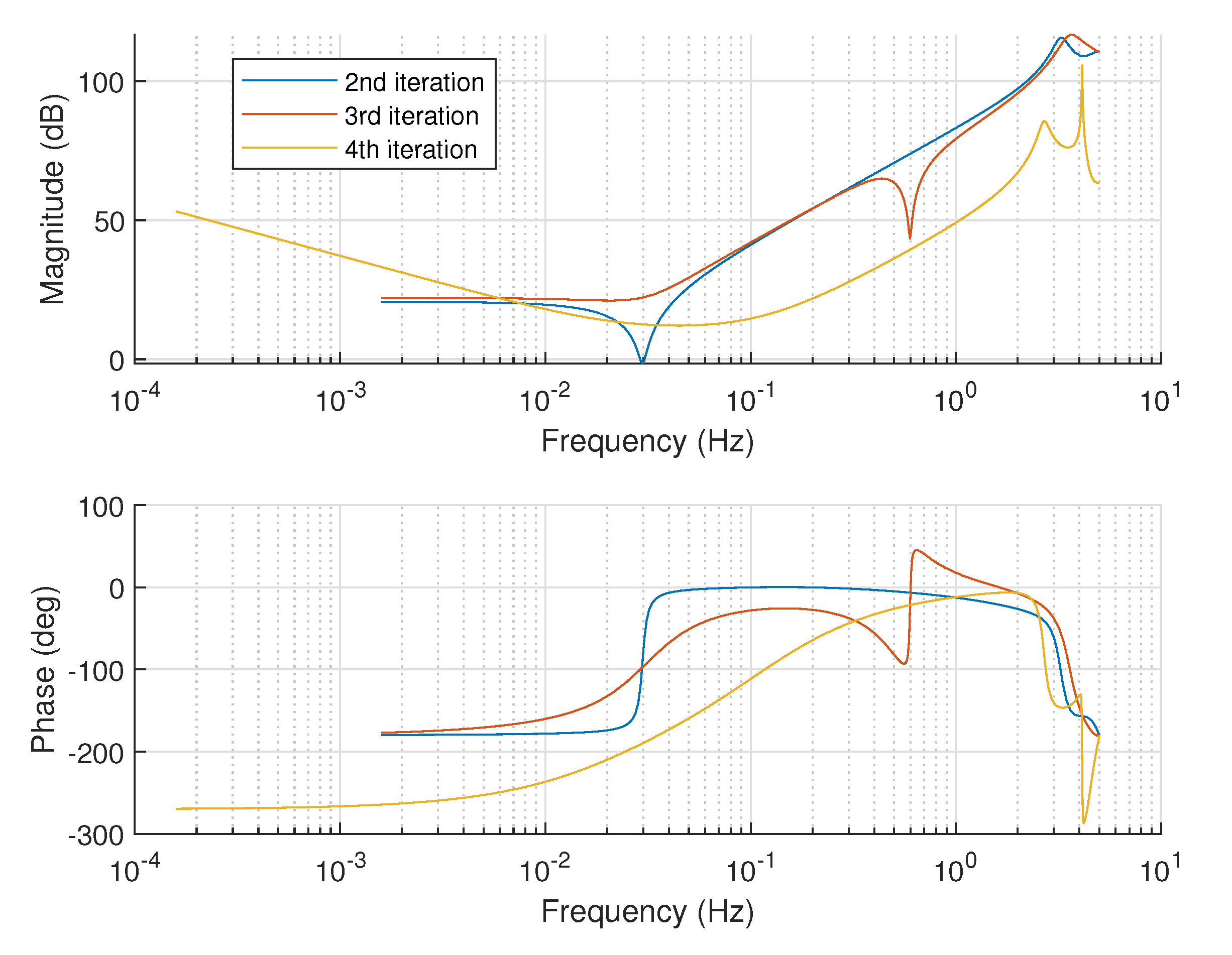
Figure 3 compares the Bode plots of the controllers from each iteration. The controllers have similar dynamics in the low-frequency range up to 0.01 Hz, and the difference between them is only in the amplification. The first-iteration controller (a pure $H_{\infty }$) is with the highest gain of about 10 dB. The 2nd- and 3rd-iteration controllers share an identical proportional action, while the 4th iteration gives a controller with smaller unit amplification of around $-10$ dB. The reduction in the proportional term can improve the system’s robust stability but can have a negative effect on robust performance. On the other hand, the controller’s action is concentrated in frequencies between 0.01 up to 1 Hz, where a pronounced resonance is observed. The controller will react to the transient changes in the blood glucose concentrations in this frequency range, i.e., minimizing their future impact. The resonant frequency from the first and second-iteration controller is about the same at 0.03 Hz. The 2nd-iteration controller band is slightly narrower around its peak compared to the first one. The third-iteration controller is more aggressive and tries to shift the resonance frequency up to 0.1 Hz, obviously aiming for faster insulin infusion in a wider range of frequencies; however, in that case, its $\mu$ value goes above 1, i.e., not all performance requirements will be satisfied. The 4th-iteration controller is an attempt to keep the resonance frequency of the 3rd controller and reduce its bandwidth, but unfortunately the structure of such a controller is not feasible because of the very high $\mu$. This can be understood by looking at the phase response where the 4th-iteration controller contains many unbalanced poles, which increase its phase delay below 200 degrees, which correlates negatively with stability.

The structure of D and $G_r$ scaling matrices obtained from the automatic optimization procedure is diagonal where $D=diag(D_1\left(j\omega \right),1,1)$ and $G_r=diag(G_{r,1}\left(j\omega \right),1,1)$. Hence, the terms $D_1$ and $G_{r,1}$ will scale the uncertainty element arising from the parameter $T_u$ representing the variable reaction of the subcutaneous BG concentration to plasma levels. The values of $D_1$ for 2nd, 3rd, and 4th iterations are plotted in Figure 4, since for the 1st iteration the D-scale is the identity matrix. And the $G_r$ term is presented in Figure 5, where it can be seen that the damping frequency for the controller from the 3rd iteration is less than the damping frequency for the controller from the 2nd iteration. For the other iterations, the $G_r$ term is zero.

4.3. Closed-Loop Performance

The sensitivity functions of the closed-loop control system with the designed $\mu$-controller from the 2nd iteration, which has the best robust metrics, satisfy the performance requirements from the specification of weighting filters $W_u$ and $W_e$. Since the controller guarantees that

$$\parallel W_e{\left(j\omega \right)S\left(j\omega \right)\parallel }_{\infty }<\gamma ,$$

(31)

where $S\left(j\omega \right)$ is the output sensitivity function, this requirement is equivalent to an upper bound constraint for the magnitude of S, determined by the inverse magnitude response of the weighting filter when $\gamma \approx 1$, i.e.,

$$\left|S\left(j\omega \right)\right|<\frac{1}{|W_e\left(j\omega \right)|}.$$

(32)

Figure 6 presents the examination of this requirement, where plots are for both the upper bound determined by $W_e$ and for the uncertain LTI closed loop with the $\mu$-controller, where the uncertain element is randomly sampled 30 times.

It is evident that the closed-loop system satisfies the weighing requirement both in the low- and high-frequency domains with a margin. The critical region where the system performance is tightly limited by the upper bound is around the cut-off frequency, which determines the response time with respect to output disturbances [38]. In this region, the majority of plant variation due to uncertainty is concentrated. If we compare this with the open loop uncertainty ranges from Figure 1, we can see that the $\mu$-controller effectively reduces the closed-loop uncertainty. The closed loop also exhibits resonance behavior around 0.02 Hz, which can be related to the level of over-dosing in case of meal events.

Similarly, for the sensitivity of the control signal to external disturbances, we have

$$\left|K\left(j\omega \right)S\left(j\omega \right)\right|<\frac{1}{|W_u\left(j\omega \right)|},$$

(33)

where K is the designed LTI controller. The comparison between the upper bound of the control sensitivity and the actual closed-loop frequency response is presented in Figure 7. Again, the closed-loop response is evaluated for 30 random samples for the introduced uncertainty element. The controller satisfies with good margin the performance requirement for the control signal u for all frequencies.

The complementary sensitivity function $T=1-S$ of the closed-loop system with the $\mu$-controller is evaluated in Figure 8, which represents the relationship between the BG target and the actual measured concentration. Here, we can measure the bandwidth of the system, which is between 0.001 and 0.01 Hz. The effect of the uncertainty over the complementary sensitivity function is to reduce its bandwidth. Depending on the variable delay between the plasma concentration and subcutaneous BG measurements, we can expect that system will respond faster or slower to maintain the BG concentration but within the limits of less than 1 decade of frequency variation. For the worst case, when the delay is largest, the controller will regulate the BG back to normal slower but still will achieve the target.

Since the controller order is 24, which might be high for implementation in digital devices, we decided to assess the possibility for its order reduction. In Figure 9 the Hankel singular values of the designed controller are shown. It is seen that the possible order of reduced controller may be selected as 10. In Figure 10, the singular values of the original and the reduced-order $\mu$-controllers are compared. They are almost the same. Therefore, it is expected that with the reduced-order controller, the achieved closed-loop performance will be similar. Finally, we evaluated the bounds of structured singular value for robust performance of the closed-loop system (Figure 11). Both controllers provide robust performance for the prescribed range of uncertainty.

5. Results and Discussion

The examination of the controller performance in the time domain was executed first with the nonlinear Hovorka model presented in Section 2. And after this, the controller was applied to the UVa/Padova simulator for the population of adult subjects. The UVa/Padova is recognized by the FDA as a benchmark software for testing AP algorithms for their acceptance in actual medical trials.

5.1. Simulation with Hovorka Model

The nonlinear Hovorka model described with Equations (1)–(5) was prepared by the authors in the MATLAB/Simulink environment as a Simulink block diagram. The states of the nonlinear model are represented with Integrator blocks, where the output of the integrator block is the state $x_i$, and the input to the integrator block is the state derivative ${\dot{x}}_i$. Then, the arithmetic relations for the calculation of the state derivatives according to the model equations are entered with the help of respective mathematical blocks. As a result, we have a plant model with two inputs and one output. The inputs are the insulin infusion rate in IUs/min and the meal intake rate in g/min equivalent carbohydrate amount. The output of the model is BG concentration measured in mg/dL. Additionally, the uncertain element $T_{unc}$ is also introduced in the model as an additional dynamic element represented as an integrator together with a feedback Gain block containing the current setting of $T_{unc}$. The designed $\mu$-controller was entered in the Simulink models with the help of the Discrete State-Space block, where the A, B, C, and D matrices from the state space realization of the controller are specified. The output of the controller is saturated to not allow negative numbers for the insulin infusion rate ($u\left(t\right)\ge 0$).

The closed-loop BG target was set to 6 mmol/L or about 105 mg/dL. The exogenous disturbance signal $d\left(t\right)$ was simulated as a pulse train signal, where each pulse duration is set to 15 min to approximate the duration of a meal. The amount of carbohydrates introduced with each meal is fixed at 100 g. Therefore, the purpose of the simulation is to verify controller performance in the presence of loading disturbances.

The results from the simulation are presented in Figure 12, which contains the output signal, and Figure 13, which contains the input signal. Because of the uncertain element in the model, we simulated the closed nonlinear system for 30 random samples of the uncertain element. From Figure 12, it is evident that the $\mu$-controller ensures the robust stability and performance of the system in the presence of the parametric uncertainty. All instances of the simulation lead to successful regulation of the BG levels after the applied disturbances. Two kinds of behavior are present. In some cases, disturbance regulation is an aperiodic process, and in other cases, it is a criticalaperiodic process. The worst-case deviation into the hypoglycemic region is above 90.

Figure 13 presents the compensation of glucose variation due to introduced meals and endogenous glucose production. The basal level of BG for the simulation was set in accordance with the operating point from the linearization of the Hovorka model. We can see that the unconstrained controller output is oscillatory. This can also be confirmed from the resonance in Figure 6 or Figure 7. When we put the non-negativity constraint over the control signal, we obtain a half period of the oscillation cut-off. The resultant reaction of the controller, when the BG is disturbed due to carbohydrate intake, is a train of oscillation half periods or boluses of insulin. Such behavior is also evident in the conventional AP controllers, which distribute the dose of insulin over time intervals instead of trying to infuse the full dose of calculated bolus. Recent research [39] revealed that 1–2 h after a meal, insulin secretion from the pancreas is not continuous—it oscillates, and the period of oscillation is about 3–6 min.

5.2. Simulation with UVa/Padova

The controller was also evaluated in the environment of the UVa/Padova simulator, which is a state-of-the-art tool for proving the feasibility of closed-loop controllers for type 1 diabetes. The controller is applied to the provided simulator group of 10 adult subjects, plus 1 subject representing an average adult population. The selected scenario is a 24 h period with an unannounced single meal equivalent to 50 g of carbohydrate intake. Detailed results are presented for all subjects in

Table 4. Result summary from the UVa/Padova simulation with the $\mu$-controller for 10 subjects from the adult population.

ID	BG	preBG	postBG	AUC	LBGI	HBGI	BGRI	SDRoC	A + B
1	125.59	124.83	165.35	95.76	0	0.63	0.63	0.3	96.18
2	123.72	123.36	148.89	62.52	0	0.44	0.44	0.23	100
3	123.35	119.39	153.82	86.63	0	0.45	0.45	0.24	92.16
4	120.77	119.46	164.45	113.76	0.01	0.5	0.51	0.34	96.81
5	124.31	121.45	161.69	110.87	0	0.6	0.6	0.31	95.49
6	117.67	115.69	169.96	120.49	0.03	0.4	0.43	0.37	100
7	120.18	114.98	174.71	155.1	0	0.58	0.59	0.41	97.43
8	134.15	130.54	175.91	124.37	0	1.33	1.33	0.35	46.22
9	114.84	113.16	163.97	123.04	0.08	0.35	0.42	0.36	100
10	113.71	113.26	148.24	84.3	0.08	0.2	0.28	0.28	100
$E(•)$	120.37	118.51	166.66	127.41	0.03	0.52	0.55	0.38	97.99

Columns: ID—subject identification, BG—blood glucose concentration in mg/dL, preBG—BG concentration before meal, postBG—BG concentration after meal, AUC—postprandial area under the curve of BG per 1 g of carbohydrates, LBGI—low blood glucose index, HBGI—high blood glucose index, BGRI—blood glucose risk index, SDRoC—standard deviation of BG rate of change, A + B—% of time in A and B zones from CVGA.

.

Several well-recognized metrics in the AP field are presented in Table 4. It is evident that the designed controller is quite successful, and all indicators are in the desired ranges. The average BG levels for all subjects are in the target zone between 70 and 180 mg/dL, even during the carbohydrate intake. The glucose regulation time is between 2 and 3 h after the meal. Low and high blood glucose indices are under 2 for all subjects. Blood glucose does not fall under 50 mg/dL, violate either low or high target bounds, or reach the excessive value of 300 mg/dL for any of the examined subjects.

The population graph trace of the BG variation for the selected scenario is presented in Figure 14, where the mean BG for the population is plotted along with minimal, maximal, and standard deviation bounds. All curves are in the range from 80 to 180 mg/dL, which is perfectly acceptable. Figure 15 presents the hourly calculated glucose risk indices where HBGI is positive number and LBGI is a negative number, along with their standard deviations taken for the examined population.

Figure 16 presents the control-variability grid analysis (CVGA) per subject of the simulated adult population. The CVGA is a powerful tool that is well accepted by AP engineers for judging the outcomes of a simulation. We see that all subjects with the $\mu$-controller fall into the green A-zone and bordering with the upper B-zone, but not intersecting into it. Figure 17 shows the CVGA when the Padova simulator is run with the reduced-order controller from the 10th order. It is seen that the result is again satisfactory, which justifies the controller order reduction. Thus, for practical implementation, we can use a simpler $\mu$-controller of the 10th order.

For more realistic results, we run the proposed controller with an additional scenario. This is a 24 h scenario with three main meals and one snack. The timings of the meals were set to 7:00, 14:00 and 20:00 with the amount of 30 g of carbohydrates without announcement. A snack was added at 16:00 with amount of 15 g. We emphasize again that the insulin bolus was not explicitly calculated due to the fact that we did not use the provided meal announcement signal from the simulator. This is the more pessimistic case for the simulation and is better for exposing controller advantages. In Figure 18 and Figure 19, we show the results from the simulation, where all subjects are in the A or B zone from the CVGA plot, and glucose levels are in the range from 80 to 270 mg/dL. This results confirm again the robust stability and performance of the controller with the high-order nonlinear model used in the Padova simulator.

6. Conclusions

The present article demonstrates the successful application of $\mu$-synthesis in the control of the AP system without explicit meal announcements. The design was based on the nonlinear Hovorka model to account for the typical adult subject with type 1 diabetes. The addition of a single uncertain element to the model effectively converts it into an infinite model set, which is a plausible description of the intersubject variability observed in the real applications. The $\mu$-controller achieves robust stability and robust performance in the whole frequency range under consideration. This was validated in a simulation with the linearized model, Hovorka model, and through the UVa/Padova simulator. The results from UVa/Padova are exceptionally good for the population of 10 adult subjects and a 24 h simulation with several meals.

The authors are well aware of the limited conclusions, which can be generalized from these preliminary results with the controller. To proceed with the controller implementation, additional studies with a larger group of simulated subjects are needed. Also, the controller should be simulated for all kinds of meal amount variations and extended simulation periods. If a practical implementation of such a controller is envisioned, it should be augmented with additional safety layers to prevent any non-simulated situations, which can lead to over- or under-dosage. Despite these recognized concerns, the $\mu$-controller shows the great potential to properly decide insulin boluses according to the worst-case estimate produced by an observer for the linearized model states. The observer inherent in the $H_{\infty }$ controller design guarantees asymptotic convergence of the error between measured BG signal and predicted BG from the model. The structure of the selected Hovorka model is matching the structure of the metabolic process. When the model states are properly estimated to establish functional matching to the process, we can be confident that the model is representing the process. Then, the state feedback term of the $\mu$-controller, which is designed to regulate the particular linearized model, will be efficient in regulating the actual glucose metabolism.

The $\mu$-controllers are typically of relatively high order, i.e., excessive computational requirements can be faced. In our case, the resultant controller is from the 24th order, which is way beyond, for example, a conventional PID-based control (second-order). This means that for every sample interval, the control algorithm must process a system of 24 differential equations with more than 500 coefficients. Hence, such a computation can pose slightly higher power requirements for the microcontroller than a conventional AP algorithm. However, that computational burden is considerably smaller than the power requirement for the communication or pump. Additionally, the controller order could be reduced by employing a model reduction technique such as examining its Hankel singular values. In this work, we reduced the controller order from 24th to 10th, and the obtained results show that the performance of the closed-loop system is not degraded.

The methods of the modern control theory, such as $\mu$-synthesis, can lead to great improvements in the design of AP systems, even when the system model is disturbed by parametric or signal uncertainties. The robust controllers like the one presented are capable of direct installation in the field with actual subjects, without the necessity for a pre-learning phase, open-loop running time, explicit meal announcement, subject-specific tuning, or a controller warm-up period.

References

1. Nakrani, M.N.; Wineland, R.H.; Anjum, F. Physiology, Glucose Metabolism. In StatPearls [Internet]; StatPearls Publishing: Treasure Island, FL, USA, 2023. Available online: https://www.ncbi.nlm.nih.gov/books/NBK560599/ (accessed on 1 June 2023).
2. American Diabetes Association. Standards of Care in Diabetes to Guide Prevention, Diagnosis, and Treatment for People Living with Diabetes; American Diabetes Association: Arlington, VA, USA, 2023. [Google Scholar]
3. National Institute for Health and Care Excellence. Type 1 Diabetes in Adults: Diagnosis and Management; National Institute for Health and Care Excellence: London, UK, 2017. [Google Scholar]
4. Pfeiffer, E.F. Artificial pancreas: State of the Art. Int. J. Artif. Organs 1988, 11, 13–26. [Google Scholar] [CrossRef]
5. Peng, Z.; Xie, X.; Tan, Q.; Kang, H.; Cui, J.; Zhang, X.; Li, W.; Feng, G. Blood glucose sensors and recent advances: A review. J. Innov. Opt. Health Sci. 2022, 15, 2230003. [Google Scholar] [CrossRef]
6. Berget, C.; Messer, L.H.; Forlenza, G.P. A Clinical Overview of Insulin Pump Therapy for the Management of Diabetes: Past, Present, and Future of Intensive Therapy. Diabetes Spectr. 2019, 32, 194–204. [Google Scholar] [CrossRef]
7. Seron, M.M.; Braslavsky, J.H.; Goodwin, G.C. Fundamental Limitations in Filtering and Control; Springer: London, UK, 1997; ISBN 9781447112440. [Google Scholar]
8. Melo, K.F.S.; Bahia, L.R.; Pasinato, B.; Porfirio, G.J.M.; Martimbianco, A.L.; Riera, R.; Calliari, L.E.P.; Minicucci, W.J.; Turatti, L.A.A.; Pedrosa, H.C.; et al. Short-acting insulin analogues versus regular human insulin on postprandial glucose and hypoglycemia in type 1 diabetes mellitus: A systematic review and meta-analysis. Diabetol Metab. Syndr. 2019, 11, 2. [Google Scholar] [CrossRef]
9. Fushimi, E.; De Battista, H.; Garelli, F. A Dual-Hormone Multicontroller for Artificial Pancreas Systems. IEEE J. Biomed. Health Inform. 2022, 26, 4743–4750. [Google Scholar] [CrossRef]
10. Olcomendy, L.; Pirog, A.; Lebreton, F.; Jaffredo, M.; Cassany, L.; Derigny, D.G.; Cieslak, J.; Henry, D.; Lang, J.; Catargi, B.; et al. Integrating an Islet-Based Biosensor in the Artificial Pancreas: In Silico Proof-of-Concept. IEEE Trans. Biomed. Eng. 2022, 69, 899–909. [Google Scholar] [CrossRef]
11. Lewis, D.; Leibrand, S. Real-World Use of Open Source Artificial Pancreas Systems. J. Diabetes Sci. Technol. 2016, 10, 1411. [Google Scholar] [CrossRef]
12. Knebel, T.; Neumiller, J.J. Medtronic MiniMed 670G Hybrid Closed-Loop System. Clin. Diabetes 2019, 37, 94–95. [Google Scholar] [CrossRef]
13. Kublin, O.; Stępień, M. The Nightscout system—Description of the system and its evaluation in scientific publications. Pediatr. Endocrinol. Diabetes Metab. 2020, 26, 140–143. [Google Scholar] [CrossRef]
14. Gomez, E.J.; Pérez, M.E.H.; Vering, T.; Cros, M.R.; Bott, O.; García-Sáez, G.; Pretschner, P.; Brugués, E.; Schnell, O.; Patte, C.; et al. The INCA System: A Further Step Towards a Telemedical Artificial Pancreas. IEEE Trans. Inf. Technol. Biomed. 2008, 12, 470–479. [Google Scholar] [CrossRef]
15. Jacobs, P.G.; El Youssef, J.; Castle, J.; Bakhtiani, P.; Branigan, D.; Breen, M.; Bauer, D.; Preiser, N.; Leonard, G.; Stonex, T.; et al. Automated Control of an Adaptive Bihormonal, Dual-Sensor Artificial Pancreas and Evaluation During Inpatient Studies. IEEE Trans. Biomed. Eng. 2014, 61, 2569–2581. [Google Scholar] [CrossRef]
16. Ramkissoon, C.M.; Aufderheide, B.; Bequette, B.W.; Vehi, J. A Review of Safety and Hazards Associated With the Artificial Pancreas. IEEE Rev. Biomed. Eng. 2017, 10, 44–62. [Google Scholar] [CrossRef] [PubMed]
17. Man, C.D.; Micheletto, F.; Lv, D.; Breton, M.; Kovatchev, B.; Cobelli, C. The UVA/PADOVA Type 1 Diabetes Simulator: New Features. J. Diabetes Sci. Technol. 2014, 8, 26–34. [Google Scholar] [CrossRef]
18. Sanz, R.; Garcia, P.; Diez, J.-L.; Bondia, J. Artificial Pancreas System With Unannounced Meals Based on a Disturbance Observer and Feedforward Compensation. IEEE Trans. Control. Syst. Technol. 2021, 29, 454–460. [Google Scholar] [CrossRef]
19. Turksoy, K.; Samadi, S.; Feng, J.; Littlejohn, E.; Quinn, L.; Cinar, A. Meal Detection in Patients With Type 1 Diabetes: A New Module for the Multivariable Adaptive Artificial Pancreas Control System. IEEE J. Biomed. Health Inform. 2016, 20, 47–54. [Google Scholar] [CrossRef]
20. Paoletti, N.; Liu, K.S.; Chen, H.; Smolka, S.A.; Lin, S. Data-Driven Robust Control for a Closed-Loop Artificial Pancreas. IEEE/ACM Trans. Comput. Biol. Bioinform. 2020, 17, 1981–1993. [Google Scholar] [CrossRef]
21. Lee, S.; Kim, J.; Park, S.W.; Jin, S.-M.; Park, S.-M. Toward a Fully Automated Artificial Pancreas System Using a Bioinspired Reinforcement Learning Design: In Silico Validation. IEEE J. Biomed. Health Inform. 2021, 25, 536–546. [Google Scholar] [CrossRef]
22. Chakrabarty, A.; Zavitsanou, S.; Doyle, F.J.; Dassau, E. Event-Triggered Model Predictive Control for Embedded Artificial Pancreas Systems. IEEE Trans. Biomed. Eng. 2018, 65, 575–586. [Google Scholar] [CrossRef]
23. Batmani, Y.; Khodakaramzadeh, S.; Moradi, P. Automatic Artificial Pancreas Systems Using an Intelligent Multiple-Model PID Strategy. IEEE J. Biomed. Health Inform. 2022, 26, 1708–1717. [Google Scholar] [CrossRef]
24. Meneghetti, L.; Terzi, M.; Favero, S.; Susto, G.A.; Cobelli, C. Data-Driven Anomaly Recognition for Unsupervised Model-Free Fault Detection in Artificial Pancreas. IEEE Trans. Control. Syst. Technol. 2020, 28, 33–47. [Google Scholar] [CrossRef]
25. Chakrabarty, A.; Healey, E.; Shi, D.; Zavitsanou, S.; Doyle, F.J.; Dassau, E. Embedded Model Predictive Control for a Wearable Artificial Pancreas. IEEE Trans. Control. Syst. Technol. 2020, 28, 2600–2607. [Google Scholar] [CrossRef]
26. Huyett, L.M.; Dassau, E.; Zisser, H.C.; Doyle, F.J. Glucose Sensor Dynamics and the Artificial Pancreas. IEEE Control. Syst. Mag. 2018, 38, 30–46. [Google Scholar] [CrossRef]
27. Bondia, J.; Romero-Vivó, S.; Ricarte, B.; Díez, J.L. Insulin Estimation and Prediction. IEEE Control. Syst. Mag. 2018, 38, 47–66. [Google Scholar]
28. Borri, A.; Cacace, F.; Gaetano, A.; Germani, A.; Manes, C.; Palumbo, P.; Panunzi, S.; Pepe, P. Observers for Nonlinear Time-Delay Systems with Application to the Artificial Pancreas. IEEE Control. Syst. Mag. 2017, 37, 33–49. [Google Scholar]
29. Ruiz-Velázquez, E.; García-Rodríguez, J.; Quiroz, G.; Femat, R. Robust μ-synthesis: Towards a unified glucose control in adults, adolescents and children with T1DM. J. Frankl. Inst. 2020, 357, 9633–9653. [Google Scholar] [CrossRef]
30. Cassany, L.; Gucik-Derigny, D.; Cieslak, J.; Henry, D.; Franco, R.; Ferreira de Loza, A.; Ríos, H.; Olcomendy, L.; Pirog, A.; Bornat, Y.; et al. A Robust H- Control Approach for Blood Glucose Regulation in Type-1 Diabetes. IFAC-PapersOnLine 2021, 54, 460–465. [Google Scholar] [CrossRef]
31. Cassany, L.; Gucik-Derigny, D.; Cieslak, J.; Henry, D.; Franco, R.; De Loza, A.F.; Rios, H.; Olçomendy, L.; Pirog, A.; Bornat, Y.; et al. A Robust Control solution for Glycaemia Regulation of Type-1 Diabetes Mellitus. In Proceedings of the 2021 European Control Conference (ECC), Delft, The Netherlands, 29 June–2 July 2021; pp. 327–332. [Google Scholar] [CrossRef]
32. Mandal, S.; Sutradhar, A. Robust controller for artificial pancreas for patients with type-1 diabetes. Res. Biomed. Eng. 2023, 39, 437–450. [Google Scholar] [CrossRef]
33. Hovorka, R.; Canonico, V.; Chassin, L.J.; Haueter, U.; Massi-Benedetti, M.; Federici, M.O.; Wilinska, M.E. Nonlinear model predictive control of glucose concentration in subjects with type 1 diabetes. Physiol. Meas. 2004, 25, 905. [Google Scholar] [CrossRef] [PubMed]
34. Bergman, R.N. Origins and History of the Minimal Model of Glucose Regulation. Front. Endocrinol. 2021, 11, 583016. [Google Scholar] [CrossRef] [PubMed]
35. Turksoy, K.; Quinn, L.; Littlejohn, E.; Cinar, A. Multivariable Adaptive Identification and Control for Artificial Pancreas Systems. IEEE Trans. Biomed. Eng. 2014, 61, 883. [Google Scholar] [CrossRef] [PubMed]
36. Zhou, K.; Doyle, J.C. Essentials of Robust Control; Prentice Hall: Hoboken, NJ, USA, 1998; ISBN 9780137908745. [Google Scholar]
37. Gu, D.-W.; Petkov, P.H.; Konstantinov, M.M. Robust Control Design with MATLAB®; Springer: London, UK, 2014; ISBN 9781447146827. [Google Scholar]
38. Doyle, J.; Francis, B.; Tannenbaum, A. Feedback Control Theory; Macmillan Publising Co.: New York, NY, USA, 1990. [Google Scholar]
39. Hellman, B.; Gylfe, E.; Grapengiesser, E.; Dansk, H.; Salehi, A. Insulin oscillations—clinically important rhythm. Antidiabetics should increase the pulsative component of the insulin release. Läkartidningen 2007, 104, 2236–2239. (In Swedish) [Google Scholar] [PubMed]
Figure 1. Frequency response of the uncertain linearization of the Hovorka model from the insulin rate to glucose concentration.
Mathematics 11 03856 g001
Figure 2. Closed-loop interconnection of the μ -controller K with the uncertain element Δ and weighting filters W e and W u .
Mathematics 11 03856 g002
Figure 3. Frequency response of the μ -controller.
Mathematics 11 03856 g003
Figure 4. Frequency response of the uncertainty D 1 element from the D-scaling matrix.
Mathematics 11 03856 g004
Figure 5. Frequency response of G r = ( I + G 2 ) 0.5 scaling.
Mathematics 11 03856 g005
Figure 6. Output sensitivity function for the 30 samples from the uncertain closed-loop system (blue) and the inverse weighting filter 1 / W e ( j ω ) (red).
Mathematics 11 03856 g006
Figure 7. Control signal sensitivity function to output disturbances for the 30 samples from the uncertain closed-loop system (blue) and the inverse weighting filter 1 / W u ( j ω ) (red).
Mathematics 11 03856 g007
Figure 8. Complementary sensitivity function of the uncertain closed loop with the μ -controller.
Mathematics 11 03856 g008
Figure 9. Hankel singular values.
Mathematics 11 03856 g009
Figure 10. Controller singular value comparison.
Mathematics 11 03856 g010
Figure 11. Robust performance comparison.
Mathematics 11 03856 g011
Figure 12. Glucose concentration from a Monte Carlo simulation with the nonlinear Hovorka model with the μ -controller.
Mathematics 11 03856 g012
Figure 13. Insulin infusion rate from a Monte Carlo simulation with the nonlinear Hovorka model with the μ -controller for 30 random samples.
Mathematics 11 03856 g013
Figure 14. Glucose trace for the 10-adult population from the UVA/Padova simulator. The green line represents the average glucose, the orange line represents the ± 1 standard deviation interval, and the red line is the minimal and maximal values from the envelope.
Mathematics 11 03856 g014
Figure 15. Glucose risk index calculated for each hour with ± 1 standard deviation confidence.
Mathematics 11 03856 g015
Figure 16. CVGA analysis for the full order μ -controller.
Mathematics 11 03856 g016
Figure 17. CVGA analysis for the reduced order μ -controller.
Mathematics 11 03856 g017
Figure 18. Glucose trace for the 10-adult population from the UVA/Padova simulator for 24 h scenario. The green line represents the average glucose, the orange line represents the ± 1 standard deviation interval, and the red line is the minimal and maximal values from the envelope.
Mathematics 11 03856 g018
Figure 19. CVGA analysis for 24 h scenario.
Mathematics 11 03856 g019