Article

Survival Analysis of a Predator–Prey Model with Seasonal Migration of Prey Populations between Breeding and Non-Breeding Regions

1
School of Date Science, Tongren University, Tongren 554300, China
2
School of Mathematical Sciences, Guizhou Normal University, Guiyang 550025, China
3
School of Electronic and Electrical Engineering, Shanghai University of Engineering Science, Shanghai 201620, China
4
School of Mathematics and Statistics, Guizhou University of Finance and Economics, Guiyang 550025, China
*
Author to whom correspondence should be addressed.
Mathematics 2023, 11(18), 3838; https://doi.org/10.3390/math11183838
Submission received: 7 August 2023 / Revised: 4 September 2023 / Accepted: 5 September 2023 / Published: 7 September 2023

Abstract

:
In this paper, we establish and study a novel predator–prey model that incorporates: (i) the migration of prey between breeding and non-breeding regions; (ii) the refuge effect of prey; and (iii) the reduction in prey pulse birth rate, in the form of a fear effect, in the presence of predators. Applying the Floquet theory and the comparison theorem of impulsive differential equations, we obtain the sufficient conditions for the stability of the prey-extinction periodic solution and the permanence of the system. Furthermore, we also study the case where the prey population does not migrate. Sufficient conditions for the stability of the prey-extinction periodic solution and the permanence are also established, and the threshold for extinction and permanence of the prey population is obtained. Finally, some numerical simulations are provided to verify the theoretical results. These results provide a theoretical foundation for the conservation of biodiversity.
MSC:
92D25; 34A37; 34D05; 37M05

1. Introduction

Migration, the seasonal round-trip movement of organisms between two (or more) locations, is ubiquitous. Migratory species are found over the earth, in terrestrial, aquatic, and aerial environments, including most vertebrates (fish, birds, mammals, amphibians, reptiles) and many invertebrate lineages [1]. In addition, many species closely related to humans are also migratory species, such as insect crop pests (Holland et al. [2]), fishery species (Parrish [3]), and ungulates competing with domestic livestock (Talbot [4]). To understand the biodynamics in population ecological management, the migration or diffusion of populations between patches has attracted the attention of many scholars, and proposed many bio-mathematical models. For example, Allen [5], Cohen and Murray [6], Zeng et al. [7], Cui et al. [8], Yang et al. [9], Takigawa [10], Freedman [11], Yan and Gao [12], and Zou and Wang [13] established and studied continuous diffusion population models using ordinary differential equations. When the individual number of species in two patches is not large enough, demographic fluctuations are often expected in the models, as stated in [14]. Studies of population models with random fluctuations and migrations between patches have attracted increasing attention in recent contributions. Zu et al. [15] discussed a single-species nonlinear diffusion system with stochastic perturbation. Zou et al. [16,17,18] studied a single-species population model with a protection zone, and they showed that protected areas can slow down the extinction speed of endangered species. Later, Wei and Wang [19] modified the model [16] and provided sustainable strategies for local managers to avoid the extinction of endangered species. Considering both white noise and Levy jump noise, Liu et al. [20] proposed and studied a logistic population model with migration. Some related studies [21,22] gave us a deeper understanding of migration patterns. Furthermore, many scholars use fractional order differential equations to establish corresponding mathematical models, which further promotes the development of population models [23,24].
In all of the above population models, the authors have always assumed that population migration occurs at any time and between any two patches simultaneously. However, the migration behavior of many species is affected by the environment, animal physiological behavior, and human activities, such as the seasonal migrations of some birds, insects, and fish [1,2]. Therefore, many scholars describe this migration phenomenon in the form of pulses in the process of modeling [25,26,27,28,29,30,31,32,33,34,35]. Global stability and persistence for impulsive migration models were studied by Huang and Yang [25], Wang et al. [26], Jiao et al. [27,28], Liu et al. [29], Shao [30], Liu and Yang [31], Liu et al. [32], Zhang et al. [33], and Wan and Jiang [34].
However, only a few studies have considered this case of periodic migration of the entire population between the patches, especially the predator–prey model with seasonal migration between breeding and non-breeding regions. We all know that mass migration of many animals can be seasonal as it is closely related to reproduction. For example, C a r i b o u is the species with the longest migration distance among land mammals. They migrate to the same location in the desolate tundra to breed each summer, and then trek south to the forest for winter [36]. M a g e l l a n i c p e n g u i n is also a common seasonal migratory animal, they leave the breeding area from March to April per year, and return to the location from August to September [36,37]. Moreover, many birds (such as S n o w g e e s e , A r c t i c t e r n , S w a n , and C i c o n i a b o y c i a n a ) breed at high latitudes in summer and fly to warm areas at low latitudes in winter [36,38]. In addition, synchronous reproduction is also a common natural phenomenon for many seasonal migrating animals (such as M o n g o l i a n g z a e l l e , W i l d e b e e s t and S n o w g e e s e ), which give birth to their cubs at almost the same time when they arrive at the breeding place. A large number of dates show that almost all pregnant female C a r i b o u will give birth between 1 and 10 June [36]. Although, migratory animals face dangers during migration, and nature still ensures that migratory animals and migration cycles exist. However, human activities can disrupt this biological status rapidly. To better protect wild animals, many countries have established numerous nature reserves to provide shelters for endangered species. It is practically significant to study the role of nature reserves from the perspective of a mathematical model.
In view of the above things, we establish and study a novel predator–prey model that incorporates: (i) the migration of prey between breeding and non-breeding regions; (ii) the refuge effect of prey; and (iii) the reduction in prey pulse birth rate, in the form of a fear effect, in the presence of predators. The organization of this article is presented below. In Section 2, we formulate our mathematical model. In Section 3, we introduce some lemmas to discuss our main results. In Section 4, we analyze the stability of the prey-extinction periodic solution and the condition for the coexistence of prey and predator, respectively. Numerical simulation and discussions are provided in Section 5. Finally, the results are summarized in Section 6.

2. Model Formulation

Let x ( t ) be the density of prey at time t. Let y ( t ) be the density of predator at time t. In this paper, we assume that prey populations migrate seasonally between the non-breeding region (Patch 1) and the breeding region (Patch 2), while predator populations always live in Patch 2. Prey x lives in Patch 2 in ( n γ , ( n + l 1 ) γ ] , when the environment in Patch 2 changes, the prey x will migrate from Patch 2 to Patch 1 in ( ( n + l 1 ) γ , ( n + l 1 + l 2 ) γ ] , when the environment in Patch 1 changes, the prey x will migrate from Patch 1 to Patch 2 in ( ( n + l 1 + l 2 + l 3 ) γ , ( n + 1 ) γ ] , where γ denotes a period of seasonal succession. 0 < l i < 1 , i = 1 , 2 , 3 and l 1 + l 3 + 2 l 2 = 1 . Figure 1 displays a diagram representing the migration process within a time-cycle.
Additional model assumptions are as follows:
(1) Prey x can be preyed upon by natural enemies and suffer unexpected losses during migration. An enormous migration team establishes a group defense effect against natural enemies. Thus, we model the mortality rate in the migration process by non-constant function μ i 1 + θ e x 1 + e x , where μ i > 0 ( i = 1 , 2 ) denotes the maximal mortality, e > 0 represents the coefficient of semi-saturation, θ ( 0 , 1 ) is the measure of the loss contrast between group and individual migrations.
(2) We assume that the prey population x has the habit of synchronous reproduction, i.e., cubs are born immediately when the prey x arrives at the breeding sites. The birth of cubs is modeled by b x ( t ) , where b is the intrinsic growth rate.
(3) To protect prey populations, we provide a refuge for prey populations and assume that prey in the refuge have an increased birth rate η > 1 . In addition, some experiments have shown that fear of predation can significantly reduce the reproduction of prey [39,40,41]. Motivated by the insightful works [39,40,41], we model the impulse birth of prey x by
x ( t + ) = x ( t ) + ( 1 m ) b x ( t ) 1 + c y ( t ) + η b m x ( t ) , t = ( n + 1 ) γ ,
where 0 < m < 1 is the proportion of prey in refuge. 1 1 + c y represents the cost of anti-predator defense owing to predation fear [40,41], c > 0 refers to the level of fear. x ( t + ) = lim h 0 + x ( t + h ) .
According to the above assumptions, we propose the following predator–prey model with seasonal migration of the prey population between breeding and non-breeding regions:
d x ( t ) d t = x ( t ) ( d 1 + a 1 x ( t ) + β ( 1 m ) y ( t ) ) , t ( n γ , ( n + l 1 ) γ ] , μ 1 1 + θ e x ( t ) 1 + e x ( t ) x ( t ) , t ( ( n + l 1 ) γ , ( n + l 1 + l 2 ) γ ] , x ( t ) ( d 2 + a 2 x ( t ) ) , t ( ( n + l 1 + l 2 ) γ , ( n + l 1 + l 2 + l 3 ) γ ] , μ 2 1 + θ e x ( t ) 1 + e x ( t ) x ( t ) , t ( ( n + l 1 + l 2 + l 3 ) γ , ( n + 1 ) γ ] , d y ( t ) d t = y ( t ) ( r 1 b 1 y ( t ) + κ β ( 1 m ) x ( t ) ) , t ( n γ , ( n + l 1 ) γ ] , y ( t ) ( r 2 b 2 y ( t ) ) , t ( ( n + l 1 ) γ , ( n + 1 ) γ ] , x ( t + ) = x ( t ) + ( 1 m ) b x ( t ) 1 + c y ( t ) + η b m x ( t ) , t = ( n + 1 ) γ ,
where r 1 and r 2 are the growth rates of predator y in the interval ( n γ , ( n + l 1 ) γ ] and ( ( n + l 1 ) γ , ( n + 1 ) γ ] , respectively. a 1 and a 2 represent the intra-specific competition coefficients of population x in the interval ( n γ , ( n + l 1 ) γ ] and ( ( n + l 1 + l 2 ) γ , ( n + l 1 + l 2 + l 3 ) γ ] , respectively. b 1 and b 2 denote the intra-specific competition coefficients of population y in the interval ( n γ , ( n + l 1 ) γ ] and ( ( n + l 1 ) γ , ( n + 1 ) γ ] , respectively. d 1 and d 2 denote the death rates of prey x in the interval ( n γ , ( n + l 1 ) γ ] and ( ( n + l 1 + l 2 ) γ , ( n + l 1 + l 2 + l 3 ) γ ] , respectively. β denotes the predation rate. κ denotes the rate of conversion of nutrients into the reproduction rate of predator.

3. Preliminaries

Let ψ ( t ) = ( x ( t ) , y ( t ) ) be the solution of Equation (1). Obviously, ψ : R + R + 2 is a piecewise continuous function where R + = { x : x 0 } and R + 2 = { ( x , y ) R 2 : x 0 , y 0 } . In light of [42], the uniqueness and global existence of solution of Equation (1) is guaranteed by the smoothness properties of g = ( g 1 , g 2 ) T , which represents the mapping defined by the right-hand side of Equation (1).
If x = 0 , we can obtain a prey-free subsystem as follows:
d y ( t ) d t = y ( t ) [ r 1 b 1 y ( t ) ] , t ( n γ , ( n + l 1 ) γ ] , y ( t ) [ r 2 b 2 y ( t ) ] , t ( ( n + l 1 ) γ , ( n + 1 ) γ ] .
The analytic solution of system (2) is given by
y ( t ) = r 1 y ( n γ ) e r 1 ( t n γ ) r 1 + b 1 y ( n γ ) ( e r 1 ( t n γ ) 1 ) , t ( n γ , ( n + l 1 ) γ ] , r 2 y ( ( n + l 1 ) γ ) e r 2 ( t ( n + l 1 ) γ ) r 2 + b 2 y ( ( n + l 1 ) γ ) ( e r 2 ( t ( n + l 1 ) γ ) 1 ) , t ( ( n + l 1 ) γ , ( n + 1 ) γ ] .
Then, the stroboscopic map of (3) is
y ( ( n + 1 ) γ ) = y ( n γ ) e ( r 1 l 1 + r 2 ( 1 l 1 ) ) γ + A y ( n γ ) ,
where A = b 1 r 1 e r 2 ( 1 l 1 ) γ ( 1 e r 1 l 1 γ ) + b 2 r 2 ( 1 e r 2 ( 1 l 1 ) γ ) . Denote y n = y ( n γ ) , then the difference equation can be derived as follows:
y n + 1 = y n e ( r 1 l 1 + r 2 ( 1 l 1 ) ) γ + A y n = h ( y n ) .
Clearly, Equation (4) has two fixed points y 0 = 0 and y * = 1 e ( r 1 l 1 + r 2 ( 1 l 1 ) ) γ A .
Lemma 1. 
The trivial fixed point of Equation (4) is unstable, and the positive fixed point y * is globally asymptotically stable.
Proof. 
From (4), we obtain
h ( y ) y y = 0 = e ( r 1 l 1 + r 2 ( 1 l 1 ) ) γ > 1 , h ( y ) y y = y * = e ( r 1 l 1 + r 2 ( 1 l 1 ) ) γ < 1 ,
thus, the trivial fixed point is unstable and the positive fixed point y * of (4) is locally asymptotically stable. And because
1 y n 1 y * = 1 y n 1 1 y * e ( r 1 ( l 1 + 2 l 2 ) + r 2 l 3 ) γ 0 a s n + ,
and y n is bounded, then | y n y * | 0 as n + , which implies that the fixed point y * is globally asymptotically stable. □
Similar to [43], we can get the following lemma.
Lemma 2. 
System (3) has a unique positive γ-periodic solution y ( t ) ¯ , and the periodic solution y ( t ) ¯ is globally asymptotically stable, where
y ( t ) ¯ = r 1 y * e r 1 ( t n γ ) r 1 + b 1 y * ( e r 1 ( t n γ ) 1 ) , t ( n γ , ( n + l 1 ) γ ] , r 2 y 1 * e r 2 ( t ( n + l 1 + l 2 ) γ ) r 2 + b 2 y 1 * ( e r 2 ( t ( n + l 1 + l 2 ) γ ) 1 ) , t ( ( n + l 1 ) γ , ( n + 1 ) γ ] ,
and
y ( 0 + ) ¯ = y * , y 1 * = r 1 y * e r 1 l 1 γ r 1 + b 1 y * ( e r 1 l 1 γ 1 ) , A = b 1 r 1 e r 2 ( 1 l 1 ) γ ( 1 e r 1 l 1 γ ) + b 2 r 2 ( 1 e r 2 ( 1 l 1 ) γ ) .
Next, we consider the following auxiliary system:
d ω ( t ) d t = d 1 ω ( t ) a 1 ω 2 ( t ) , t ( n γ , ( n + l 1 ) γ ] , θ μ 1 ω ( t ) , t ( ( n + l 1 ) γ , ( n + l 1 + l 2 ) γ ] , d 2 ω ( t ) a 2 ω 2 ( t ) , t ( ( n + l 1 + l 2 ) γ , ( n + l 1 + l 2 + l 3 ) γ ] , θ μ 2 ω ( t ) , t ( ( n + l 1 + l 2 + l 3 ) γ , ( n + 1 ) γ ] , ω ( t + ) = [ 1 + ( ( 1 m ) + η m ) b ] ω ( t ) , t = ( n + 1 ) γ , n Z + .
Assumption : h 0 = ( 1 + ( ( 1 m ) + η m ) b ) e ( d 1 l 1 + θ μ 1 l 2 + d 2 l 3 + θ μ 2 l 2 ) γ .
Lemma 3. 
(i) If h 0 1 , we have lim t + ω ( t ) = 0 .
(ii) If h 0 > 1 , system (5) has a unique globally asymptotically stable positive periodic solution ω ( t ) ¯ , where
ω ( t ) ¯ = d 2 ω * e d 1 ( t n γ ) d 1 + a 1 ω * ( 1 e d 1 ( t n γ ) ) , t ( n γ , ( n + l 1 ) γ ] , ω 1 * e μ 1 θ ( t ( n + l 1 ) γ ) , t ( ( n + l 1 ) γ , ( n + l 1 + l 2 ) γ ] , d 2 ω 2 * e d 2 ( t ( n + l 1 + l 2 ) γ ) d 2 + a 2 ω 2 * ( 1 e d 1 ( t ( n + l 1 + l 2 ) γ ) ) , t ( ( n + l 1 + l 2 ) γ , ( n + l 1 + l 2 + l 3 ) γ ] , ω 3 * e μ 2 θ ( t ( n + l 1 + l 2 + l 3 ) γ ) , t ( ( n + l 1 + l 2 + l 3 ) γ , ( n + 1 ) γ ] ,
and
ω * = h 0 1 B , ω 1 * = d 1 ω * e d 1 l 1 γ d 1 + a 1 ω * ( 1 e d 1 l 1 γ ) , ω 2 * = ω 1 * e μ 1 θ l 2 γ ) , ω 3 * = d 2 ω 2 * e d 2 l 3 γ d 2 + a 2 ω 2 * ( 1 e d 2 l 3 γ ) ,
B = a 2 d 2 e ( d 1 l 1 + μ 1 θ l 2 ) γ ( 1 e d 2 l 3 γ ) + a 1 d 1 ( 1 e d 1 l 1 γ ) .
Proof. 
The analytic solution of system (5) is
ω ( t ) = d 1 ω ( n γ + ) e d 1 ( t n γ ) d 1 + a 1 ω ( n γ + ) ( 1 e d 1 ( t n γ ) ) , t ( n γ , ( n + l 1 ) γ ] , ω ( ( n + l 1 ) γ ) e μ 1 θ ( t ( n + l 1 ) γ ) , t ( ( n + l 1 ) γ , ( n + l 1 + l 2 ) γ ] , d 2 ω ( ( n + l 1 + l 2 ) γ ) e d 2 ( t ( n + l 1 + l 2 ) γ ) d 2 + a 2 ω ( ( n + l 1 + l 2 ) γ ) ( 1 e d 2 ( t ( n + l 1 + l 2 ) γ ) ) , t ( ( n + l 1 + l 2 ) γ , ( n + l 1 + l 2 + l 3 ) γ ] , ω ( ( n + l 1 + l 2 + l 3 ) γ ) e μ 1 θ ( t ( n + l 1 + l 2 + l 3 ) γ ) , t ( ( n + l 1 + l 2 + l 3 ) γ , ( n + 1 ) γ ] .
Then, the stroboscopic map of (6) is presented by
ω ( ( n + 1 ) γ + ) = h 0 ω ( n γ + ) 1 + B ω ( n γ + ) ,
where B = a 2 d 2 e ( d 1 l 1 + μ 1 θ l 2 ) γ ( 1 e d 2 l 3 γ ) + a 1 d 1 ( 1 e d 1 l 1 γ ) . Denote ω n = ω ( n γ + ) , we can obtain the following difference equation:
ω n + 1 = h 0 ω n 1 + B ω n = g ( ω n ) .
Obviously, function g ( ω ) is a strictly increasing function and g ( ω ) ω is a strictly decreasing function.
(i) When h 0 1 , it follows from (7) that ω n + 1 < h 0 ω n ω n , thus, { ω n } is a strictly decreasing and bounded sequence, this implies that { ω n } converges to ω 0 0 . From (7), we obtain that ω 0 = g ( ω 0 ) , and calculate that ω 0 = 0 , which also implies that lim t + ω ( t ) = 0 when h 0 1 .
(ii) When h 0 > 1 , Equation (7) has two fixed points ω 0 = 0 and ω * = h 0 1 B . By calculation, we have
g ( ω ) ω ω = 0 = h 0 > 1 , g ( ω ) ω ω = ω * = 1 h 0 < 1 ,
thus, the trivial fixed point is unstable, and the positive fixed point ω * is locally asymptotically stable. Moreover,
1 ω n 1 ω * = 1 h 0 1 ω n 1 1 ω * 0 a s n + ,
and ω n is bounded, then | ω n ω * | 0 as n + , which means that the fixed point ω * is globally asymptotically stable. Similar to [43], system (5) has a globally asymptotically stable positive periodic solution
ω ( t ) ¯ = d 2 ω * e d 1 ( t n γ ) d 1 + a 1 ω * ( 1 e d 1 ( t n γ ) ) , t ( n γ , ( n + l 1 ) γ ] , ω 1 * e μ 1 θ ( t ( n + l 1 ) γ ) , t ( ( n + l 1 ) γ , ( n + l 1 + l 2 ) γ ] , d 2 ω 2 * e d 2 ( t ( n + l 1 + l 2 ) γ ) d 2 + a 2 ω 2 * ( 1 e d 1 ( t ( n + l 1 + l 2 ) γ ) ) , t ( ( n + l 1 + l 2 ) γ , ( n + l 1 + l 2 + l 3 ) γ ] , ω 3 * e μ 2 θ ( t ( n + l 1 + l 2 + l 3 ) γ ) , t ( ( n + l 1 + l 2 + l 3 ) γ , ( n + 1 ) γ ] ,
and
ω 1 * = d 1 ω * e d 1 l 1 γ d 1 + a 1 ω * ( 1 e d 1 l 1 γ ) , ω 2 * = ω 1 * e μ 1 θ l 2 γ , ω 3 * = d 2 ω 2 * e d 2 l 3 γ d 2 + a 2 ω 2 * ( 1 e d 2 l 3 γ ) .
The proof is complete. □
Remark 1. 
From Lemma 3 and the comparison theorem, we obtain that x ( t ) ω ( t ) max { 0 , ω * } + ϵ for ϵ > 0 small enough and t large enough.
Lemma 4. 
Let ω ( t ) ¯ be the positive periodic solution of system (5), then
l 1 γ ( l 1 + l 2 ) γ μ 1 1 + θ e ω ( t ) ¯ 1 + e ω ( t ) ¯ d t = μ 1 l 2 γ + 1 θ θ ln 1 + e ω 1 * exp ( μ 1 θ l 2 γ ) 1 + e ω 1 * ,
( l 1 + l 2 + l 3 ) γ γ μ 2 1 + θ e ω ( t ) ¯ 1 + e ω ( t ) ¯ d t = μ 2 l 2 γ + 1 θ θ ln 1 + e ω 3 * exp ( μ 2 θ l 2 γ ) 1 + e ω 3 * .
Proof. 
From Lemma 3, we obtain that
l 1 γ ( l 1 + l 2 ) γ μ 1 1 + θ e ω ( t ) ¯ 1 + e ω ( t ) ¯ d t = l 1 γ ( l 1 + l 2 ) γ μ 1 μ 1 ( 1 θ ) e ω ( t ) ¯ 1 + e ω ( t ) ¯ d t = μ 1 l 2 γ + 1 θ θ l 1 γ ( l 1 + l 2 ) γ d ( e ω ( t ) ¯ + 1 ) 1 + e ω ( t ) ¯ = μ 1 l 2 γ + 1 θ θ ln 1 + e ω 1 * exp ( μ 1 θ l 2 γ ) 1 + e ω 1 * .
Similarly,
( l 1 + l 2 + l 3 ) γ γ μ 2 1 + θ e ω ( t ) ¯ 1 + e ω ( t ) ¯ d t = μ 2 l 2 γ + 1 θ θ ln 1 + e ω 3 * exp ( μ 2 θ l 2 γ ) 1 + e ω 3 * .
The proof is complete. □
Lemma 5. 
For any solution ψ ( t ) of system (1) with ψ ( 0 ) > 0 , system (1) is bounded for t large enough.
Proof. 
It follows from Remark 1 that for any ϵ > 0 , there always exist a n 0 Z + such that 0 x ( t ) < max { ω * , 0 } + ϵ for t n 0 γ . Denote r ˜ = max { r 1 , r 2 + max { ω * , 0 } + ϵ } and b ˜ = min { b 1 , b 2 } . From (1), we have
d y ( t ) d t y ( t ) ( r ˜ b ˜ y ( t ) ) , t n 0 γ ,
then there must be a M 1 > 0 such that y ( t ) < M 1 for t large enough. □

4. Main Results

Denote
h 1 = 1 + ( 1 m ) b 1 + c y * + η m b e d 1 l 1 γ μ 1 l 2 γ d 2 l 3 γ μ 2 l 2 γ 0 l 1 γ β ( 1 m ) y ( s ) ¯ d s
and
h 2 = ( 1 + ( 1 m ) b 1 + c y * + η m b ) exp { ( d 1 l 1 + d 2 l 3 ) γ μ 1 l 1 γ ( l 1 + l 2 ) γ 1 + θ e ω ( t ) ¯ 1 + e ω ( t ) ¯ d t μ 2 ( l 1 + l 2 + l 3 ) γ γ 1 + θ e ω ( t ) ¯ 1 + e ω ( t ) ¯ d t ( 1 m ) β 0 l 1 γ y ( t ) ¯ d t } .
According to Lemmas 2 and 4, we can obtain that
h 1 = 1 + ( 1 m ) b 1 + c y * + η m b e ( d 1 l 1 + μ 1 l 2 + d 2 l 3 + μ 2 l 2 ) γ β ( 1 m ) 0 l 1 γ r 1 y * e r 1 t r 1 + b 1 y * ( e r 1 t 1 ) d t = 1 + ( 1 m ) b 1 + c y * + η m b e ( d 1 l 1 + μ 1 l 2 + d 2 l 3 + μ 2 l 2 ) γ β ( 1 m ) b 1 ln ( e r 1 l 1 γ 1 ) y * b 1 + r 1 r 1 = 1 + ( 1 m ) b 1 + c y * + η m b 1 + b 1 y * ( e r 1 l 1 γ 1 ) r 1 β ( 1 m ) b 1 e ( d 1 l 1 + ( μ 1 + μ 2 ) l 2 + d 2 l 3 ) γ
and
h 2 = h 1 e μ 1 l 1 γ ( l 1 + l 2 ) γ 1 + θ e ω ( t ) ¯ 1 + e ω ( t ) ¯ d t μ 2 ( l 1 + l 2 + l 3 ) γ γ 1 + θ e ω ( t ) ¯ 1 + e ω ( t ) ¯ d t + μ 1 l 2 γ + μ 2 l 2 γ = h 1 1 + e ω 1 * 1 + e ω 1 * exp ( μ 1 θ l 2 γ ) 1 θ θ 1 + e ω 3 * 1 + e ω 3 * exp ( μ 2 θ l 2 γ ) 1 θ θ ,
where y * , ω 1 * and ω 3 * are given in Lemmas 2 and 3.

4.1. Stability of Prey-Extinction Periodic Solution

Theorem 1. 
The prey-extinction periodic solution ( 0 , y ( t ) ¯ ) of system (1) is locally asymptotically stable if h 1 < 1 .
Proof. 
To prove the local asymptotic stability of periodic solution ( 0 , y ( t ) ¯ ) , we discuss the behavior of small-amplitude perturbation of the solution. Define
u ( t ) = x ( t ) , v ( t ) = y ( t ) y ( t ) ¯ .
Then the linearized system of system (1) in ( n γ , ( n + 1 ) γ ] is obtained by
d u ( t ) d t = ( d 1 + β ( 1 m ) y ( t ) ¯ ) u ( t ) , d v ( t ) d t = κ β ( 1 m ) y ( t ) ¯ u ( t ) + ( r 1 2 b 1 y ( t ) ¯ ) v ( t ) , t ( n γ , ( n + l 1 ) γ ] ,
and
d u ( t ) d t = μ 1 u ( t ) , d v ( t ) d t = ( r 2 2 b 2 y ( t ) ¯ ) v ( t ) , t ( ( n + l 1 ) γ , ( n + l 1 + l 2 ) γ ] ,
and
d u ( t ) d t = d 2 u ( t ) , d v ( t ) d t = ( r 2 2 b 2 y ( t ) ¯ ) v ( t ) , t ( ( n + l 1 + l 2 ) γ , ( n + l 1 + l 2 + l 3 ) γ ] ,
and
d u ( t ) d t = μ 2 u ( t ) , d v ( t ) d t = ( r 2 2 b 2 y ( t ) ¯ ) v ( t ) , t ( ( n + l 1 + l 2 + l 3 ) γ , ( n + 1 ) γ ] ,
The fundamental solution matrix can be calculated as follows:
ϕ 1 ( t ) = e n γ t d 1 + β ( 1 m ) y ( s ) ¯ d s 0 * e n γ t r 1 2 b 1 y ( s ) ¯ d s , t ( n γ , ( n + l 1 ) γ ] ,
and
ϕ 2 ( t ) = e μ 1 ( t ( n + l 1 ) γ ) 0 0 e ( n + l 1 ) γ t r 2 2 b 2 y ( s ) ¯ d s , t ( ( n + l 1 ) γ , ( n + l 1 + l 2 ) γ ] ,
and
ϕ 3 ( t ) = e d 1 ( t ( n + l 1 + l 2 ) γ ) 0 0 e ( n + l 1 + l 2 ) γ t r 2 2 b 2 y ( s ) ¯ d s , t ( ( n + l 1 + l 2 ) γ , ( n + l 1 + l 2 + l 3 ) γ ] ,
and
ϕ 4 ( t ) = e μ 2 ( t ( n + l 1 + l 2 + l 3 ) γ ) 0 0 e ( n + l 1 + l 2 + l 3 ) γ t r 2 2 b 2 y ( s ) ¯ d s , t ( ( n + l 1 + l 2 + l 3 ) γ , ( n + 1 ) γ ] .
The exact expression for ∗ is not provided here since it is not utilized in the subsequent calculation.
The linearization of the seventh equation of system (1) is
u ( ( n + 1 ) γ + ) v ( ( n + 1 ) γ + ) = 1 + ( 1 m ) b 1 + c y * + η m b 0 0 1 u ( ( n + 1 ) γ ) v ( ( n + 1 ) γ ) .
According to the Floquet theory, we know that the prey-extinction periodic solution ( 0 , y ( t ) ¯ ) is locally asymptotically stable if the absolute values of all eigenvalues of matrix
Φ = 1 + ( 1 m ) b 1 + c y * + η m b 0 0 1 ϕ 1 ( l 1 γ ) ϕ 2 ( ( l 1 + l 2 ) γ ) ϕ 3 ( ( l 1 + l 2 + l 3 ) γ ) ϕ 4 ( γ )
are less than 1, and the eigenvalues of matrix Φ are
λ 1 = ( 1 + ( 1 m ) b 1 + c y * + η m b ) e d 1 l 1 γ μ 1 l 2 γ d 2 l 3 γ μ 2 l 2 γ 0 l 1 γ β ( 1 m ) y ( s ) ¯ d s ,
λ 2 = e 0 l 1 γ r 1 2 b 1 y ( s ) ¯ d s + l 1 γ γ r 2 2 b 2 y ( s ) ¯ d s = e ( b 1 0 l 1 γ y ( s ) ¯ d s + b 2 l 1 γ γ y ( s ) ¯ d s ) < 1 .
We can obtain that λ 1 < 1 when h 1 < 1 . Thus, the periodic solution ( 0 , y ( t ) ¯ ) of system (1) is locally asymptotically stable when h 1 < 1 . □
In the following, we study the global asymptotic stability of the periodic solution ( 0 , y ( t ) ¯ ) .
Theorem 2. 
If h 0 1 or h 0 > 1 and h 2 < 1 , the prey-extinction periodic solution ( 0 , y ( t ) ¯ ) of system (1) is globally asymptotically stable.
Proof. 
In Theorem 1, we proved the local asymptotic stability of the periodic solution ( 0 , y ( t ) ¯ ) . In the following, we simply prove that the periodic solution ( 0 , y ( t ) ¯ ) is a global attractor.
If h 0 1 , it follows from Lemma 3 that lim t + x ( t ) = 0 .
If h 0 > 1 , from (1), we have
d y ( t ) d t y ( t ) [ r 1 b 1 y ( t ) ] , t ( n γ , ( n + l 1 ) γ ] , d y ( t ) d t = y ( t ) [ r 2 b 2 y ( t ) ] , t ( ( n + l 1 ) γ , ( n + 1 ) γ ] .
According to the comparison theorem, Lemmas 2 and 3, we obtain that for all ϵ > 0 , there is a N 0 Z + such that
x ( t ) ω ( t ) ω ( t ) ¯ + ϵ , y ( t ) y ( t ) ¯ ϵ ,
for t N 0 γ . Further, we obtain that for t N 0 γ ,
d x ( t ) d t = ( d 1 + β ( 1 m ) ( y ( t ) ¯ ϵ ) ) x ( t ) , t ( n γ , ( n + l 1 ) γ ] , d x ( t ) d t μ 1 1 + θ e ( ω ( t ) ¯ + ϵ ) 1 + e ( ω ( t ) ¯ + ϵ ) x ( t ) , t ( ( n + l 1 ) γ , ( n + l 1 + l 2 ) γ ] , d x ( t ) d t d 2 x ( t ) , t ( ( n + l 1 + l 2 ) γ , ( n + l 1 + l 2 + l 3 ) γ ] , d x ( t ) d t μ 2 1 + θ e ( ω ( t ) ¯ + ϵ ) 1 + e ( ω ( t ) ¯ + ϵ ) x ( t ) , t ( ( n + l 1 + l 2 ) γ , ( n + l 1 + l 2 + l 3 ) γ ] , x ( t + ) ( 1 + ( 1 m ) b 1 + c ( y * ϵ ) + η m b ) x ( t ) , t = ( n + 1 ) γ .
Integrating (10) from n γ to ( n + 1 ) γ , we obtain
x ( ( n + 1 ) γ + ) ρ x ( n γ + ) ,
where
ρ = ( 1 + ( 1 m ) b 1 + c ( y * ϵ ) + η m b ) exp { ( d 1 l 1 + d 2 l 3 ) γ μ 1 l 1 γ ( l 1 + l 2 ) γ 1 + θ e ( ω ( t ) ¯ + ϵ ) 1 + e ( ω ( t ) ¯ + ϵ ) d t μ 2 ( l 1 + l 2 + l 3 ) γ γ 1 + θ e ( ω ( t ) ¯ + ϵ ) 1 + e ( ω ( t ) ¯ + ϵ ) d t ( 1 m ) β 0 l 1 γ y ( t ) ¯ ϵ d t } ( 1 + ( 1 m ) b 1 + c ( y * ϵ ) + η m b ) 1 + b 1 y * ( e r 1 l 1 γ 1 ) r 1 β ( 1 m ) b 1 e ( d 1 l 1 + d 2 l 3 + ( μ 1 + μ 2 ) ) γ 1 + e ω 1 * 1 + e ω 1 * exp ( μ 1 θ l 2 γ ) 1 θ θ 1 + e ω 3 * 1 + e ω 3 * exp ( μ 2 θ l 2 γ ) 1 θ θ e ( μ 1 l 2 + β l 1 ) γ ϵ .
Since h 2 < 1 , we can select a ϵ > 0 small enough such that ρ < 1 . From (11), we can imply that x ( t ) 0 as t + ( n + ) , that is, for any ϵ 1 > 0 , there is a N 1 ( > N 0 ) Z + such that x ( t ) ϵ 1 for t N 1 γ . Further from (1), we have
d y ( t ) d t y ( t ) [ r 1 + κ β ( 1 m ) ϵ 1 b 1 y ( t ) ] , t ( n γ , ( n + l 1 ) γ ] , d y ( t ) d t = y ( t ) [ r 2 b 2 y ( t ) ] , t ( ( n + l 1 ) γ , ( n + 1 ) γ ] ,
for all t N 1 γ . According to the comparison theorem and Lemma 2, we obtain y ( t ) z ( t ) for t N 1 γ , and for any sufficiently small ϵ 2 > 0 , there is a N 2 > N 1 such that
z ( t ) z ( t ) ¯ + ϵ 2 , f o r t N 2 γ ,
where z ( t ) is the solution of the following comparison system
d z ( t ) d t = z ( t ) [ r 1 + κ β ( 1 m ) ϵ 1 b 1 z ( t ) ] , t ( n γ , ( n + l 1 ) γ ] , z ( t ) [ r 2 b 2 z ( t ) ] , t ( ( n + l 1 ) γ , ( n + 1 ) γ ] ,
with initial value z ( N 1 γ ) = y ( N 1 γ ) , and
z ( t ) ¯ = ( r 1 + κ β ( 1 m ) ϵ 1 ) z * e ( r 1 + κ β ( 1 m ) ϵ 1 ) ( t n γ ) ( r 1 + κ β ( 1 m ) ϵ 1 ) + b 1 z * ( e ( r 1 + κ β ( 1 m ) ϵ 1 ) ( t n γ ) 1 ) , t ( n γ , ( n + l 1 ) γ ] , r 2 z 1 * e r 2 ( t ( n + l 1 + l 2 ) γ ) r 2 + b 2 z 1 * ( e r 2 ( t ( n + l 1 + l 2 ) γ ) 1 ) , t ( ( n + l 1 ) γ , ( n + 1 ) γ ] ,
and
z ( N 1 γ + ) ¯ = z * = 1 e ( r 1 + κ β ( 1 m ) ϵ 1 ) l 1 γ + r 2 ( 1 l 2 ) γ A 1 ,
z 1 * = ( r 1 + κ β ( 1 m ) ϵ 1 ) z * e ( r 1 + κ β ( 1 m ) ϵ 1 ) l 1 γ r 1 + κ β ( 1 m ) ϵ 1 + b 1 z * ( e ( r 1 + κ β ( 1 m ) ϵ 1 ) l 1 γ 1 ) ,
A 1 = b 1 ( r 1 + κ β ( 1 m ) ϵ 1 ) e r 2 ( 1 l 1 ) γ ( 1 e ( r 1 + κ β ( 1 m ) ϵ 1 ) l 1 γ ) + b 2 r 2 ( 1 e r 2 ( 1 l 1 ) γ ) .
From (9) and (13), we get
y ( t ) ¯ ϵ y ( t ) z ( t ) ¯ + ϵ 2 , f o r t N 2 γ .
Letting ϵ 0 , ϵ 1 0 , ϵ 2 0 , we can imply that y ( t ) y ( t ) ¯ as t + . The proof is completed. □

4.2. Permanence

Theorem 3. 
If h 1 > 1 , system (1) is permanent, that is, there are L > 0 and M > 0 such that L < x ( t ) < M and L < y ( t ) < M for t large enough.
Proof. 
It follows from Lemma 5 that there exists a M > 0 such that x ( t ) M and y ( t ) M for sufficiently large t. Without loss of generality, we suppose that x ( t ) M and y ( t ) M for t 0 .
From (9), we have
y ( t ) y ( t ) ¯ ϵ min t [ 0 , γ ] y ( t ) ¯ ϵ , f o r t N 0 γ .
Choosing ϵ = 0.5 min t [ 0 , γ ] y ( t ) ¯ , we have y ( t ) 0.5 min t [ 0 , γ ] y ( t ) ¯ = L 2 for t N 0 γ , hence, predator y is always permanent.
In the following, we prove that there is a L 1 ̲ > 0 such that x ( t ) > L 1 ̲ for sufficiently large t.
If h 1 > 1 , by the continuity of solutions with respect to parameters, we select L 1 > 0 and ϵ 1 > 0 small enough such that
σ = ( 1 + ( 1 m ) b 1 + c ( Y * + ϵ 1 ) + η m b ) e ( d 1 + a 1 L 1 ) l 1 γ μ 1 l 2 γ ( d 2 + a 2 L 1 ) l 3 γ μ 2 l 2 γ β ( 1 m ) 0 l 1 γ Y ( s ) ¯ + ϵ 1 d s > 1 ,
where Y ( t ) ¯ is given (15) below.
We first prove x ( t ) < L 1 can not hold for all t 0 , if not,
d y ( t ) d t y ( t ) [ r 1 + κ β ( 1 m ) L 1 b 1 y ( t ) ] , t ( n γ , ( n + l 1 ) γ ] .
Consider the following comparison system
d Y ( t ) d t = Y ( t ) [ r 1 + κ β ( 1 m ) L 1 b 1 Y ( t ) ] , t ( n γ , ( n + l 1 ) γ ] , Y ( t ) [ r 2 b 2 Y ( t ) ] , t ( ( n + l 1 ) γ , ( n + 1 ) γ ] ,
with Y ( 0 ) = y ( 0 ) > 0 . From Lemma 2, we know that System (14) has a globally asymptotically stable periodic solution
Y ( t ) ¯ = ( r 1 + κ β ( 1 m ) L 1 ) Y * e ( r 1 + κ β ( 1 m ) L 1 ) ( t n γ ) ( r 1 + κ β ( 1 m ) L 1 ) + b 1 z * ( e ( r 1 + κ β ( 1 m ) L 1 ) ( t n γ ) 1 ) , t ( n γ , ( n + l 1 ) γ ] , r 2 Y 1 * e r 2 ( t ( n + l 1 + l 2 ) γ ) r 2 + b 2 Y 1 * ( e r 2 ( t ( n + l 1 + l 2 ) γ ) 1 ) , t ( ( n + l 1 ) γ , ( n + 1 ) γ ] ,
and
Y * = 1 e ( r 1 + κ β ( 1 m ) L 1 ) l 1 γ + r 2 ( 1 l 2 ) γ A 2 , Y 1 * = ( r 1 + κ β ( 1 m ) L 1 ) z * e ( r 1 + κ β ( 1 m ) L 1 ) l 1 γ r 1 + κ β ( 1 m ) L 1 + b 1 Y * ( e ( r 1 + κ β ( 1 m ) L 1 ) l 1 γ 1 ) ,
A 2 = b 1 ( r 1 + κ β ( 1 m ) L 1 ) e r 2 ( 1 l 1 ) γ ( 1 e ( r 1 + κ β ( 1 m ) L 1 ) l 1 γ ) + b 2 r 2 ( 1 e r 2 ( 1 l 1 ) γ ) .
By the comparison theorem, we have
y ( t ) Y ( t ) Y ( t ) ¯ + ϵ 1 f o r t n 0 γ .
From (1) and (16), we derive that for t n 0 γ ,
d x ( t ) d t = ( d 1 + a 1 L 1 + β ( 1 m ) ( Y ( t ) ¯ + ϵ 1 ) ) x ( t ) , t ( n γ , ( n + l 1 ) γ ] , d x ( t ) d t μ 1 x ( t ) , t ( ( n + l 1 ) γ , ( n + l 1 + l 2 ) γ ] , d x ( t ) d t ( d 2 + a 2 L 1 ) x ( t ) , t ( ( n + l 1 + l 2 ) γ , ( n + l 1 + l 2 + l 3 ) γ ] , d x ( t ) d t μ 2 x ( t ) , t ( ( n + l 1 + l 2 + l 3 ) γ , ( n + 1 ) γ ] , x ( t + ) ( 1 + ( 1 m ) b 1 + c ( Y * + ϵ 1 ) + η m b ) x ( t ) , t = ( n + 1 ) γ .
Integrating (17) from n γ to ( n + 1 ) γ , we have
x ( ( n + 1 ) γ + ) x ( n γ + ) σ , f o r n > n 0 ,
further,
x ( ( n + 1 ) γ + ) x ( x ( n 0 γ + ) ) σ n n 0 + , n + ,
this contradicts the boundedness of x, thus there exists a t 1 > n 0 γ such that x ( t 1 ) L 1 .
Two cases should be considered.
Case a : If x ( t ) L 1 for all t n 0 γ , the proof is complete.
Case b : x ( t ) is oscillatory about L 1 for t large enough. Let t ¯ = inf t t 1 { t : x ( t ) < L 1 } , then there must be n 1 Z + such that t ¯ [ n 1 γ , ( n 1 + 1 ) γ )   ( n 1 > n 0 ) . Clearly, x ( t ) L 1 for t [ t 1 , t ¯ ] . Since x ( t ) is a monotonically decreasing function on the interval [ n γ , ( n + 1 ) γ ) , we obtain x ( t ¯ ) = L 1 and x ( t ¯ + ) > L 1 if t ¯ = n 1 γ . If t ¯ n 1 γ , we get x ( t ¯ ) = L 1 .
Choose p Z + large enough such that
p > n 0 , ( 1 + ( 1 m ) b 1 + c M + η m b ) n 0 + 1 e d ¯ ( n 0 + 1 ) σ p n 0 > 1 ,
where d ¯ = max { d 1 + a 1 M + β ( 1 m ) M , d 2 + a 2 M , μ 1 , μ 2 } .
We claim that there must be a t 2 [ ( n 1 + 1 ) γ , ( n 1 + 1 + p ) γ ) such that x ( t 2 + ) > L 1 . Otherwise, x ( t ) < L 1 for t [ ( n 1 + 1 ) γ , ( n 1 + 1 + p ) γ ) . Letting Y ( ( n 1 + 1 ) γ ) = y ( 0 ) , we obtain from (14)–(16) that y ( t ) Y ( t ) ¯ + ϵ 1 for t ( n 1 + 1 + n 0 ) γ . From (18), we have
x ( ( n 1 + p + 1 ) γ + ) x ( ( n 1 + 1 + n 0 ) γ + ) σ p n 0 .
Because
d x ( t ) d t ( d 1 + a 1 M + β ( 1 m ) M ) x ( t ) , t ( n γ , ( n + l 1 ) γ ] , d x ( t ) d t μ 1 x ( t ) , t ( ( n + l 1 ) γ , ( n + l 1 + l 2 ) γ ] , d x ( t ) d t ( d 2 + a 2 M ) x ( t ) , t ( ( n + l 1 + l 2 ) γ , ( n + 1 + l 1 + l 2 + l 3 ) γ ] , d x ( t ) d t μ 2 x ( t ) , t ( ( n + 1 + l 1 + l 2 + l 3 ) γ , ( n + 1 ) γ ] ,
from (19), we have
d x ( t ) d t d ¯ x ( t ) , t ( ( n + l 1 + l 2 + l 3 ) γ , ( n + 1 + l 1 + l 2 + l 3 ) γ ] , x ( t + ) ( 1 + ( 1 m ) b 1 + c M + η m b ) x ( t ) , t = ( n + l 1 + l 2 + l 3 ) γ
Integrating above inequality on the interval [ t ¯ , n 1 + 1 + n 0 ] , we have
x ( ( n 1 + 1 + n 0 ) γ ) x ( t ¯ ) ( 1 + ( 1 m ) b 1 + c M + η m b ) n 0 e d ¯ ( n 0 + 1 ) = L 1 ( 1 + ( 1 m ) b 1 + c M + η m b ) n 0 e d ¯ ( n 0 + 1 ) .
And
x ( ( n 1 + p + 1 ) γ + ) x ( ( n + 1 + n 0 ) γ + ) σ p n 0 L 1 ( 1 + ( 1 m ) b 1 + c M + η m b ) n 0 + 1 e d ¯ ( n 0 + 1 ) σ p n 0 > L 1 ,
which is a contradiction. Therefore, we know that there exists t 2 > ( n 1 + 1 ) γ such that x ( t 2 + ) > L 1 . We further conclude that x ( t ) > e d ( p + 1 ) γ L 1 = L 1 ̲ for t ( t 1 , t 2 ] .
We can continue the same discussion for t t 2 since x ( t 2 + ) > L 1 . Therefore, x ( t ) L 1 ̲ for t large enough. □
If the seasonal migration of species x is not considered, the system (1) will degenerate into the following a predator–prey system with impulsive birth, fear effects and refuge effects.
d x ( t ) d t = x ( t ) [ d 0 a 0 x ( t ) β ( 1 m ) y ( t ) ] , d y ( t ) d t = y ( t ) [ r 0 b 0 y ( t ) + κ β ( 1 m ) x ( t ) ] , t ( n γ , ( n + 1 ) γ ] , x ( t + ) = ( 1 + ( 1 m ) b 1 + c y ( t ) + η m b ) x ( t ) , y ( t + ) = y ( t ) , t = ( n + 1 ) γ .
We assume in model (20) that r 0 , a 0 , d 0 , b 0 , α , β , κ , b are positive constants, 0 m 1 and η > 1 .
It is easy to obtain that the system (20) has a prey-extinction periodic solution ( 0 , r 0 b 0 ) . Denote
h 3 = ( 1 + ( 1 m ) b b 0 b 0 + c r 0 + η m b ) e ( d 0 + ( 1 m ) β r 0 b 0 ) γ .
By adopting the same proof methods as Theorems 1–3, we can also derive the following results:
Theorem 4. 
(1) If h 3 < 1 , the prey-extinction periodic solution ( 0 , r 0 b 0 ) of System (20) is globally asymptotically stable.
(2) If h 3 > 1 , system (20) is permanent.
Remark 2. 
From Theorem 4, we can easily see that h 3 is the threshold for the permanence and extinction of the prey population in System (20), that is, the prey x of System (20) will be extinct if h 3 < 1 , and the prey x is permanent if h 3 > 1 .

5. Numerical Simulations

As shown by the above theorems, it is crucial to gain a better understanding of how the refuge effect and fear effect impact the survival of migratory species. We present numerical simulations using the Matlab R2017b software to verify our theoretical results. Fixed parameters
d 1 = 0.15 , a 1 = 0.011 , r 1 = 0.1 , b 1 = 0.4 , μ 1 = 0.3 , μ 2 = 0.3 , e = 5.1 , d 2 = 0.15 , a 2 = 0.01 , θ = 0.2 , r 2 = 0.7 , b 2 = 0.6 , κ = 0.8 , β = 1.2 , b = 2 , η = 3 , γ = 4 , l 1 = 0.32 , l 2 = 0.18 , l 3 = 0.32 .

5.1. The Role of the Refuge Effect

First, by setting m = 0.45 and c = 0.1 , we can calculate that
h 1 = 1 + ( 1 m ) b 1 + c y * + η m b 1 + b 1 y * ( e r 1 l 1 γ 1 ) r 1 β ( 1 m ) b 1 e ( d 1 l 1 + ( μ 1 + μ 2 ) l 2 + d 2 l 3 ) γ = 1 + 1.1 1 + 0.1 × 1.0847 + 2.7 1 + 0.15 × 1.0847 ( e 0.128 1 ) 0.1 0.66 0.4 e 0.4704 0.9629 < 1
and
h 2 = h 1 1 + e ω 1 * 1 + e ω 1 * exp ( μ 1 θ l 2 γ ) 1 θ θ 1 + e ω 3 * 1 + e ω 3 * exp ( μ 2 θ l 2 γ ) 1 θ θ 0.9629 1 + 5.1 × 34.6397 1 + 5.1 × 34.6397 × e 0.0432 4 1 + 5.1 × 19.7493 1 + 5.1 × 19.7493 e 0.0432   ) 4 0.9629 × 1.1874 × 1.1866 1.3567 > 1 .
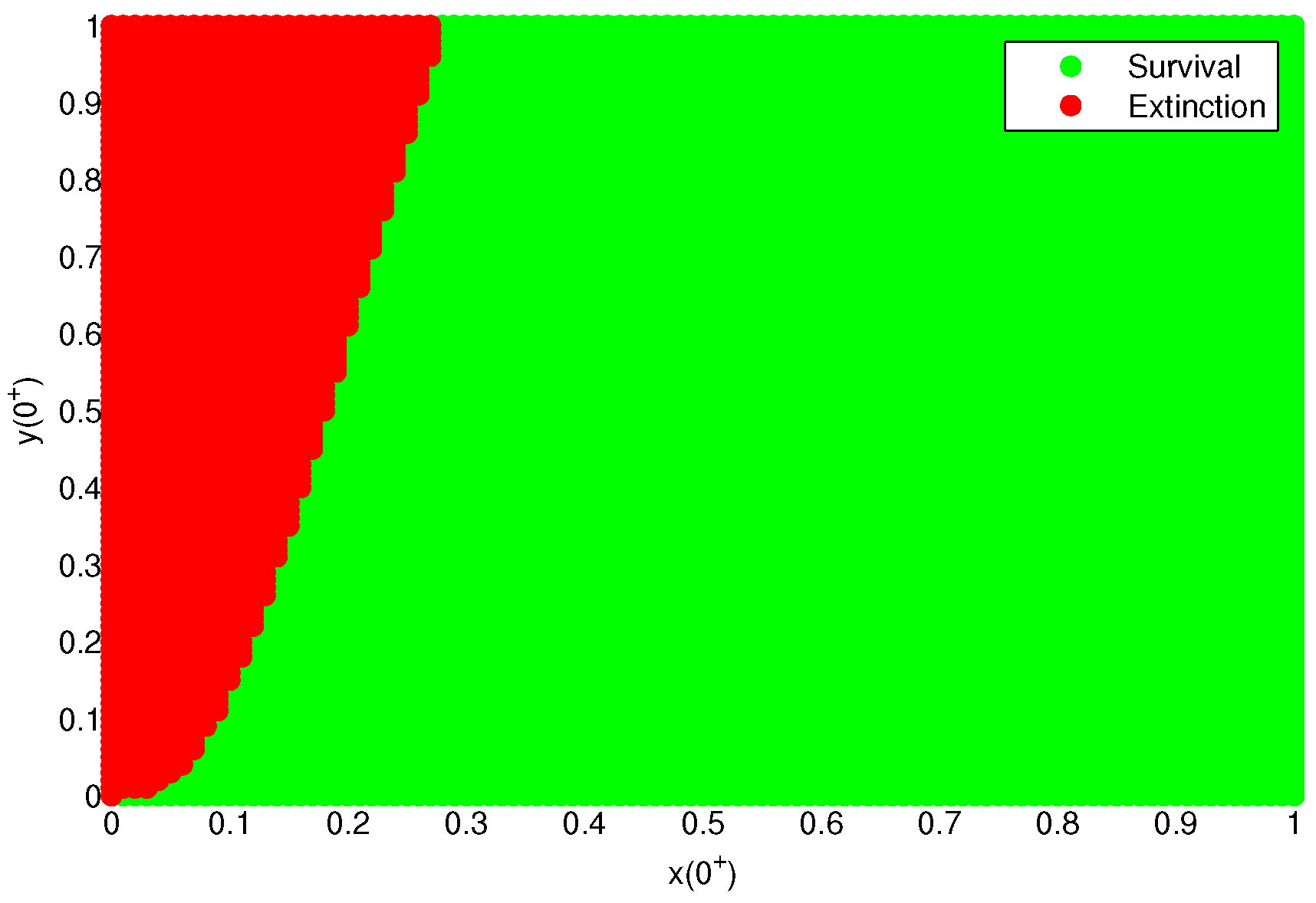
It follows from Theorem 1 that the prey-extinction periodic solution ( 0 , y ( t ) ¯ ) is locally asymptotically stable as shown in Figure 2 and Figure 3. Figure 2 reveals the phase diagrams for the survival and extinction of the prey population for different initial values ( x ( 0 + ) , y ( 0 + ) ) [ 0 , 1 ] × [ 0 , 1 ] , where the red region in Figure 2 is a region of attraction for the periodic solution of prey-extinction. In addition, we can also observe from Figure 3 that System (1) has two steady states: the prey-extinction periodic solution where the prey population goes extinct, and a positive periodic solution where both the prey and predator populations oscillate periodically and positively.
Moreover, when we take a smaller refuge effect intensity of m = 0.3 , and other parameters remain unchanged, by calculating, we have
h 2 = h 1 1 + e ω 1 * 1 + e ω 1 * exp ( μ 1 θ l 2 γ ) 1 θ θ 1 + e ω 3 * 1 + e ω 3 * exp ( μ 2 θ l 2 γ ) 1 θ θ 0.6762 × 1.1873 × 1.1864 0.9526 < 1 ,
System (1) has a unique globally asymptotically stable prey-extinction periodic solution as shown in Figure 4a, that is, the prey population will eventually become extinct for any initial value ( x ( 0 + ) , y ( 0 + ) ) R + 2 . If we choose a larger refuge effect intensity of m = 0.5 , the calculation yields
h 1 = 1 + 1 1 + 0.1 × 1.0847 + 3 1 + 0.15 × 1.0847 ( e 0.128 1 ) 0.1 3 2 e 0.4704 1.0787 > 1
from Theorem 3, we obtain that System (1) is permanent (see Figure 4b).

5.2. The Role of the Fear Effect

According to Theorems 1–3, we can confirm that the fear effect is detrimental to the permanence of the prey population in System (1). In the following, we take into account the following four cases of c: (i) c = 0.5 , (i) c = 0.8 , (iii) c = 1.2 , (iv) c = 2 . The other parameters are the same as in Figure 4b and the initial value ( x ( 0 + ) , y ( 0 + ) ) = ( 0.1 , 1 ) . Figure 5 shows that the density of the prey population will shift from a high-density state to a low-density state or even extinction as the value of c increases.

5.3. The Dynamic Behaviors of System (20)

In the following, we consider the dynamic behaviors of the prey–predator System (20) where the prey population does not migrate. Given the parameters of System (20):
d 0 = 0.15 , a 0 = 0.01 , r 0 = 0.2 , b 0 = 0.6 , β = 1.2 , κ = 0.8 , b = 2 , η = 3 , γ = 4 , c = 0.4 ,
and then vary the value of m. We first give m = 0.3 , and calculate that
h 3 = 1 + ( 1 m ) b b 0 b 0 + c r 0 + η m b e ( d 0 + ( 1 m ) β r 0 b 0 ) γ = 1 + 1.4 1 + 0.4 ÷ 3 + 1.8 e 1.72 0.7226 < 1 .
We can see from Theorem 4 that System (20) has a unique prey-extinction periodic solution ( 0 , 1 3 ) , which is globally asymptotically stable as shown in Figure 6a. When m = 0.5 , it can be calculated that
h 3 = 1 + 1 1 + 0.4 ÷ 3 + 3 e 1.4 1.204 > 1 ,
by Theorem 4, we obtain that System (20) is permanent (see Figure 6b).

6. Discussion

In Section 4, we obtain conditions for the local asymptotic stability and global asymptotic stability of the prey-extinction periodic solution, as well as for the persistence of the system. The numerical verification is carried out in Section 5 (see Figure 3, Figure 4 and Figure 6). From the proof of Theorem 2, it is easy to see that the condition for global asymptotic stability of the prey-extinction periodic solution is only a sufficient condition. If h 1 < 1 < h 2 , the prey-extinction periodic solution is locally asymptotically stable by Theorems 1 and 2. From Figure 2 and Figure 3, we observe an interesting situation that the prey population may persist when x ( 0 + ) is large enough and y ( 0 + ) is small enough. Unfortunately, for this phenomenon, we are currently limited to numerical simulations and are unable to use existing mathematical methods to give the domain of attraction for the prey-extinction periodic solution. Of course, the parameter 0 < θ < 1 plays an important role for this scenario to occur. As can be seen from the expression of h 2 , h 2 decreases as θ decreases. In particular, if θ = 1 , i.e., the effect of group migration on the population is not taken into account, then it follows from Theorems 1 and 2 that the prey-extinction periodic solution is globally asymptotically stable when h 1 < 1 . Combined with Theorem 3, this leads to the conclusion that h 1 is a threshold for extinction and persistence of prey populations.
In Model (1), we consider the effects of the refuge effect and the fear effect on the survival of prey populations. According to the expression of h 1 , we can conclude that the value of h 1 increases as m increases or c decreases. In other words, increasing the proportion of refuges or reducing the fear level of prey towards predators is favorable for the conservation of the prey population (see Figure 3, Figure 4 and Figure 5). Furthermore, in Theorem 3, we have only explored the permanence of the system (1), but as can be seen from Figure 4 and Figure 5, there exists a positive periodic solution to System (1). However, we have not yet found a good mathematical method to address the existence of the positive periodic solution, which is one of our future research directions. Future work can also modify Model (1) on the basis of model (1), such as introducing stochastic perturbations of environmental factors into Model (1) [19,22] and considering the migration of predator populations [27].

7. Conclusions

In this work, we establish and study a novel predator–prey model that incorporates: (i) the migration of prey between breeding and non-breeding areas; (ii) the refuge effect of prey; and (iii) the reduction in the prey pulse birth rate, in the form of fear effect, in the presence of predator. By applying the Floquet theory and the comparison theorem of impulsive differential equations, sufficient conditions for the stability of the prey-extinction periodic solution and the permanence of the system (1) are obtained. The study shows that the the prey refuge effect and the fear effect play a crucial role on the survival of the prey population. Furthermore, we have also investigated the case in which the prey population does not migrate (see System (20)). Sufficient conditions for the stability of the prey-extinction periodic solution and the permanence of System (20) are also established, and the threshold for extinction and permanence of the prey population is obtained.

Author Contributions

Writing—original draft preparation, Supervision, Conceptualization, X.D.; software, H.J.; funding acquisition, writing—review and editing, J.J.; validation, Q.Q. All authors have read and agreed to the published version of the manuscript.

Funding

This work is supported by the National Natural Scientific Fund of China (No. 12261018).

Data Availability Statement

Not applicable.

Acknowledgments

The authors thank the editor and anonymous referees for useful comments that led to a great improvement of the paper.

Conflicts of Interest

The authors declare no conflict of interest.

References

  1. Dingle, H. Migration: The Biology of Life on the Move, 2nd ed.; Oxford University Press: Oxford, UK, 2014. [Google Scholar]
  2. Holland, R.A.; Wikelski, M.; Wilcove, D.S. How and why do insects migrate? Science 2006, 313, 794–796. [Google Scholar] [CrossRef] [PubMed]
  3. Parrish, B.B. Fish Migration. Nature 1968, 220, 1008–1009. [Google Scholar] [CrossRef]
  4. Talbot, L.M.; Talbot, M.H. The wildebeest in western masailand, east africa. Wildl. Monogr. 1963, 12, 3–88. [Google Scholar]
  5. Allen, L.J.S. Persistence and extinction in single-species reaction-diffusion models. Bull. Math. Biol. 1983, 45, 209–227. [Google Scholar] [CrossRef]
  6. Cohen, D.S.; Murray, J.D. A generalized diffusion model for growth and dispersal in a population. J. Math. Biol. 1981, 12, 237–249. [Google Scholar] [CrossRef]
  7. Zeng, G.Z.; Chen, L.S.; Chen, J.F. Persistence and periodic orbits for two-species nonautonomous diffusion lotka-volterra models. Math. Comput. Model. 1994, 20, 69–80. [Google Scholar] [CrossRef]
  8. Cui, J.; Takeuchi, Y.; Lin, Z. Permanence and extinction for dispersal population systems. J. Math. Anal. Appl. 2004, 298, 73–93. [Google Scholar] [CrossRef]
  9. Yang, Z.; Lu, Q.; Yang, Z. The effect of diffusion on the permanence of Smith population model in a polluted patch. Commun. Nonlinear Sci. 2001, 217–221. [Google Scholar] [CrossRef]
  10. Takigawa, S. A predator–prey diffusion model in age-dependent population dynamics. Hiroshima Math. J. 1989, 19, 225–242. [Google Scholar] [CrossRef]
  11. Freedman, H.I. Single species migration in two habitats: Persistence and extinction. Math. Model. 1987, 8, 778–780. [Google Scholar] [CrossRef]
  12. Yan, Z.; Gao, S. Analysis of a nonautonomous Gompertz population growth model with dispersal in a polluted environment. J. Appl. Math. Comput. 2012, 39, 459–472. [Google Scholar]
  13. Zou, X.; Wang, K. A robustness analysis of biological population models with protection zone. Appl. Math. Model. 2011, 35, 5553–5563. [Google Scholar] [CrossRef]
  14. Ovaskainen, O.; Meerson, B. Stochastic models of population extinction. Trends Ecol. Evol. 2010, 25, 643–652. [Google Scholar] [CrossRef] [PubMed]
  15. Zu, L.; Jiang, D.; O’egan, D. Stochastic permanence, stationary distribution and extinction of a single-species nonlinear diffusion system with random perturbation. Abstr. Appl. Anal. 2014, 2014, 320460. [Google Scholar] [CrossRef]
  16. Zou, X.; Fan, D.; Wang, K. Effects of dispersal for a logistic growth population in random environments. Abstr. Appl. Anal. 2013, 2013, 912579. [Google Scholar] [CrossRef]
  17. Zou, X.; Wang, K.; Liu, M. Can protection zone potentially strengthen protective effects in random environments ? Appl. Math. Comput. 2014, 231, 26–38. [Google Scholar] [CrossRef]
  18. Zou, X.; Wang, K. Dynamical properties of a biological population with a protected area under ecological uncertainty. Appl. Math. Model. 2015, 39, 6273–6284. [Google Scholar] [CrossRef]
  19. Wei, F.Y.; Wang, C.J. Survival analysis of a single-species population model with fluctuations and migrations between patches. Appl. Math. Model. 2020, 81, 113–127. [Google Scholar] [CrossRef]
  20. Liu, M.; Deng, M.; Du, B. Analysis of a stochastic logistic model with diffusion. Appl. Math. Comput. 2015, 266, 169–182. [Google Scholar] [CrossRef]
  21. Wei, F.Y.; Chen, L.H. Psychological effect on single-species population models in a polluted environment. Math. Biosci. 2017, 290, 22–30. [Google Scholar] [CrossRef]
  22. Dai, X.; Wang, S.; Xiong, W. Survival analysis of a stochastic delay single-species system in polluted environment with psychological effect and pulse toxicant input. Adv. Differ. Equ. 2020, 2020, 604. [Google Scholar] [CrossRef]
  23. Anggriani, N.; Panigoro, H.; Rahmi, E.; Peter, O.J.; Jose, S.A. A predator–prey model with additive Allee effect and intraspecific competition on predator involving Atangana-Baleanu-Caputo derivative. Results Phys. 2023, 49, 106489. [Google Scholar] [CrossRef]
  24. Joseph, D.; Ramachandran, R.; Alzabut, J.; Jose, S.A.; Khan, H. A fractional-order density-dependent mathematical model to find the better strain of wolbachia. Symmetry 2023, 15, 845. [Google Scholar] [CrossRef]
  25. Huang, L.; Yang, Z. Dynamical behaviors of a stage-structured predator–prey model with harvesting effort and impulsive diffusion. Discret. Dyn. Nat. Soc. 2015, 2015, 371852. [Google Scholar] [CrossRef]
  26. Wang, L.; Liu, Z.; Jing, H.; Cheng, L. Impulsive diffusion in single species model. Chaos Solitons Fract. 2007, 33, 1213–1219. [Google Scholar] [CrossRef]
  27. Jiao, J.; Yang, X.; Cai, S.; Cheng, L. Dynamical analysis of a delayed predator–prey model with impulsive diffusion between two patches. Math. Comput. Simulat. 2010, 80, 522–532. [Google Scholar] [CrossRef]
  28. Jiao, J.; Cai, S. Dynamics of a new delayed stage-structured predator–prey model with impulsive diffusion and releasing. Adv. Differ. Equ. 2016, 2016, 318. [Google Scholar] [CrossRef]
  29. Liu, Z.; Teng, Z.; Zhang, L. Two patches impulsive diffusion periodic single-species logistic model. Int. J. Biomath. 2010, 3, 127–141. [Google Scholar] [CrossRef]
  30. Shao, Y. Analysis of a delayed predator–prey system with impulsive diffusion between two patches. Math. Comput. Model. 2010, 52, 120–127. [Google Scholar] [CrossRef]
  31. Liu, Z.; Yang, C. Permanence and periodic solutions for a two-patch impulsive migration periodic N-species Lotka-Volterra competitive system. Discret. Dyn. Nat. Soc. 2015, 2015, 293050. [Google Scholar] [CrossRef]
  32. Liu, Z.; Zhong, S.; Yin, C. Two-patches prey impulsive diffusion periodic predator–prey model. Commun. Nonlinear. Sci. 2011, 16, 2641–2655. [Google Scholar] [CrossRef]
  33. Zhang, L.; Teng, Z. The dynamical behavior of a predator–prey system with Gompertz growth function and impulsive dispersal of prey between two patches. Math. Method. Appl. Sci. 2016, 39, 3623–3639. [Google Scholar] [CrossRef]
  34. Wan, H.; Jiang, H. Dynamical behaviors of a predator–prey system with prey impulsive diffusion and dispersal delay between two patches. Adv. Differ. Equ. 2019, 2019, 191. [Google Scholar] [CrossRef]
  35. Jose, S.A.; Ramachandran, R.; Cao, J.; Alzabut, J.; Niezabitowski, M.; Balas, V. Stability analysis and comparative study on different eco-epidemiological models: Stage structure for prey and predator concerning impulsive control. Optim. Control Appl. Meth. 2022, 43, 842–866. [Google Scholar] [CrossRef]
  36. Hoare, B. Animal Migration: Remarkable Journeys in the Wild; University of California Press: Oakland, CA, USA, 2009. [Google Scholar]
  37. Stokes, D.L.; Boersma, P.D.; Javier, L. Conservation of migratory Magellanic penguins requires marine zoning. Biol. Conserv. 2014, 170, 151–161. [Google Scholar] [CrossRef]
  38. Jahn, A.E.; Levey, D.J.; Smith, K.G. Reflections across hemispheres: A system-wide approach to new world bird migration. Auk 2004, 121, 1005–1013. [Google Scholar] [CrossRef]
  39. Wang, X.; Zanette, L.; Zou, X. Modelling the fear effect in predator–prey interactions. J. Math. Biol. 2016, 73, 1179–1204. [Google Scholar] [CrossRef] [PubMed]
  40. Sasmal, S.K. Population dynamics with multiple allee effects induced by fear factors-a mathematical study on prey-predator interactions. Appl. Math. Model. 2018, 64, 1–14. [Google Scholar] [CrossRef]
  41. Wang, X.; Zou, X. Modeling the fear effect in predator–prey interactions with adaptive avoidance of predators. Bull. Math. Biol. 2017, 79, 1325–1359. [Google Scholar] [CrossRef] [PubMed]
  42. Lakshmikantham, V. Theory of Impulsive Differential Equations; World Scientific: Singapore, 1989. [Google Scholar]
  43. Jiao, J.; Cai, S.; Li, L. Dynamics of a periodic switched predator–prey system with impulsive harvesting and hibernation of prey population. J. Frankl. Inst. 2016, 353, 3818–3834. [Google Scholar] [CrossRef]
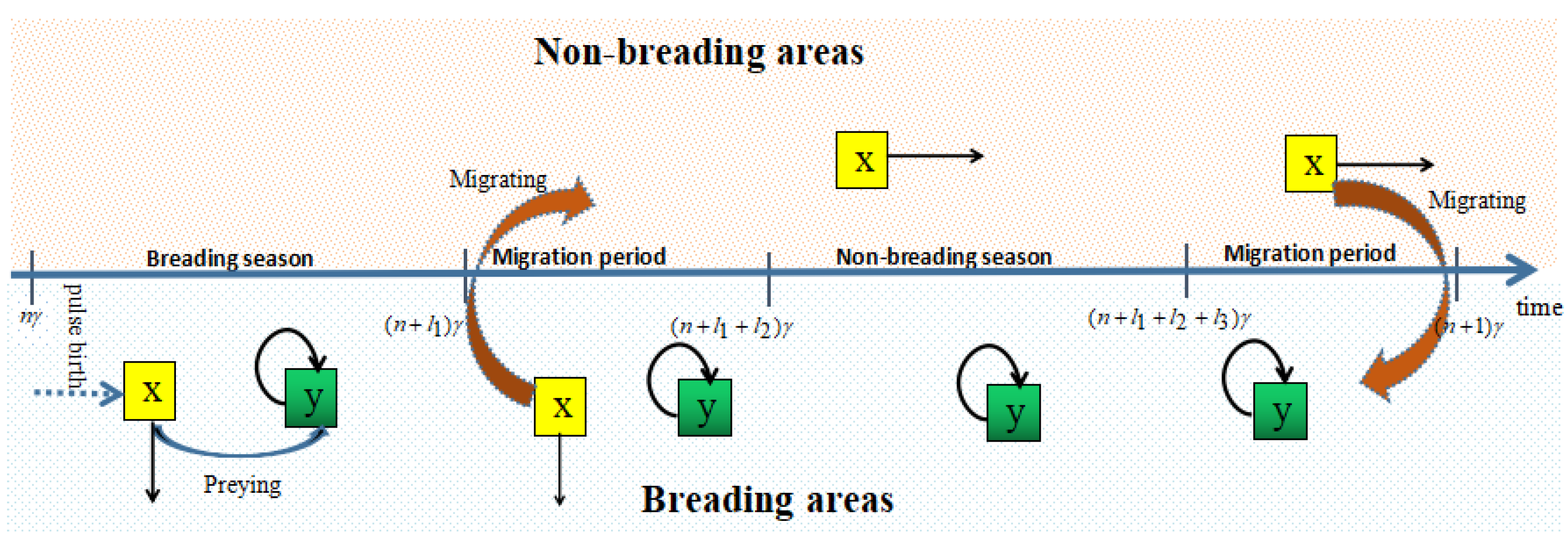
Figure 1. Schematic representation of prey migration.
Mathematics 11 03838 g001
Figure 2. The phase diagram shows whether the prey population goes to persist or trends to extinction with different initial value ( x ( 0 + ) , y ( 0 + ) ) [ 0 , 1 ] × [ 0 , 1 ] . .
Mathematics 11 03838 g002
Figure 3. The solutions of System (1) for different initial values ( x ( 0 + ) , y ( 0 + ) ) with m = 0.45 , c = 0.1 . (a): The initial value ( x ( 0 + ) , y ( 0 + ) ) takes (0.1, 0.6), (0.2, 0.8); (b): The initial value ( x ( 0 + ) , y ( 0 + ) ) takes (0.2, 0.1), (0.5, 1).
Mathematics 11 03838 g003
Figure 4. The solutions of System (1) for different refuge effect intensities m = 0.3 , 0.5 , and other parameters are the same as in Figure 2. (a): m = 0.3 , the prey-extinction periodic solution of System (1) is globally asymptotically stable; (b): m = 0.5 , System (1) is permanent.
Mathematics 11 03838 g004
Figure 5. The solutions of System (1) with different fear effect intensities c = 0.5 , 0.8 , 1.2 , 2 . Other parameters are the same as in Figure 4b.
Mathematics 11 03838 g005
Figure 6. Time series of System (20) with different refuge effect intensities m = 0.3 , 0.5 . (a): m = 0.3 , the prey-extinction periodic solution of System (20) is globally asymptotically stable; (b): m = 0.5 , System (20) is permanent.
Mathematics 11 03838 g006
Disclaimer/Publisher’s Note: The statements, opinions and data contained in all publications are solely those of the individual author(s) and contributor(s) and not of MDPI and/or the editor(s). MDPI and/or the editor(s) disclaim responsibility for any injury to people or property resulting from any ideas, methods, instructions or products referred to in the content.