
Probabilistic Slope Stability Analysis of Mount St. Helens Using Scoops3D and a Hybrid Intelligence Paradigm

 ,
, 
Abstract
:1. Introduction
2. Research Significance
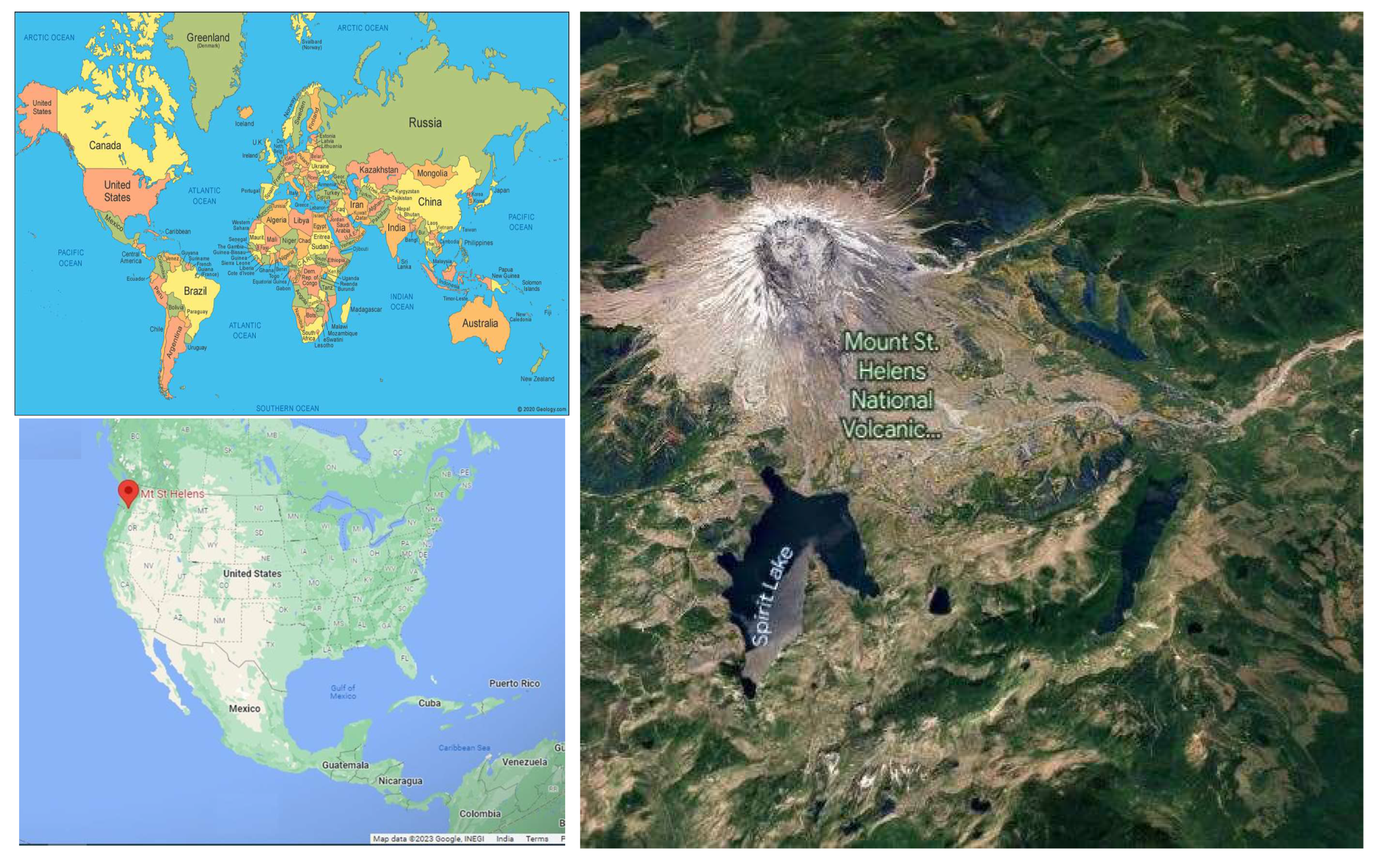
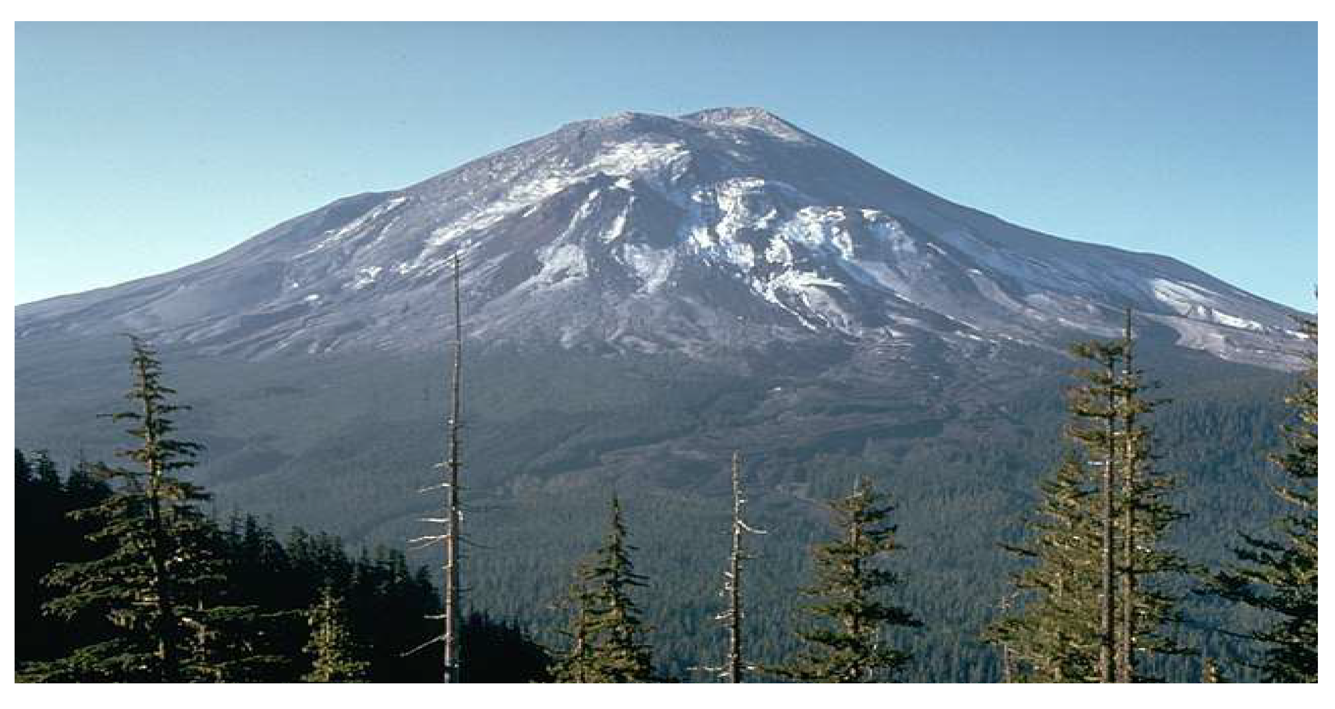
3. Study Area
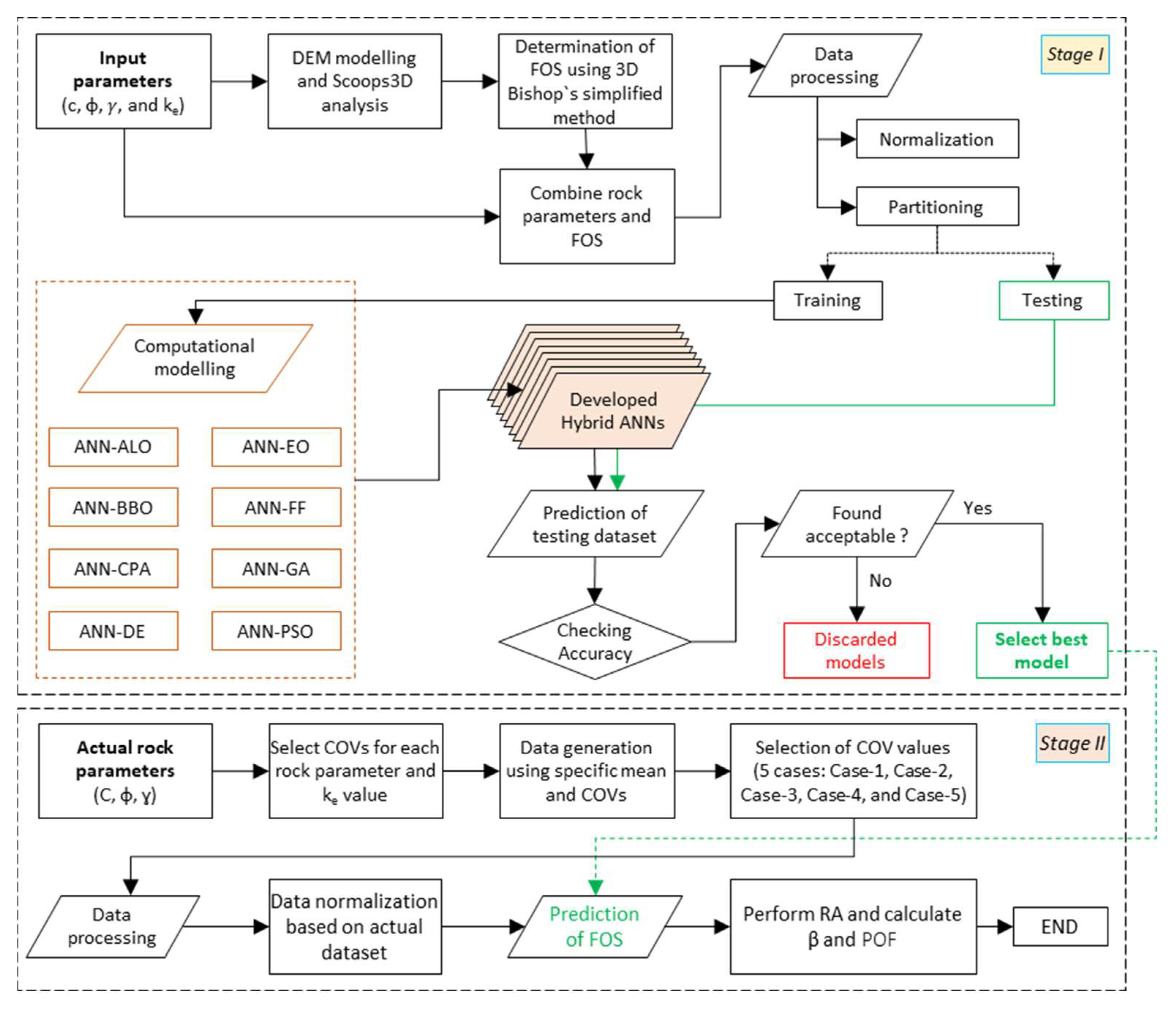
4. Methodology
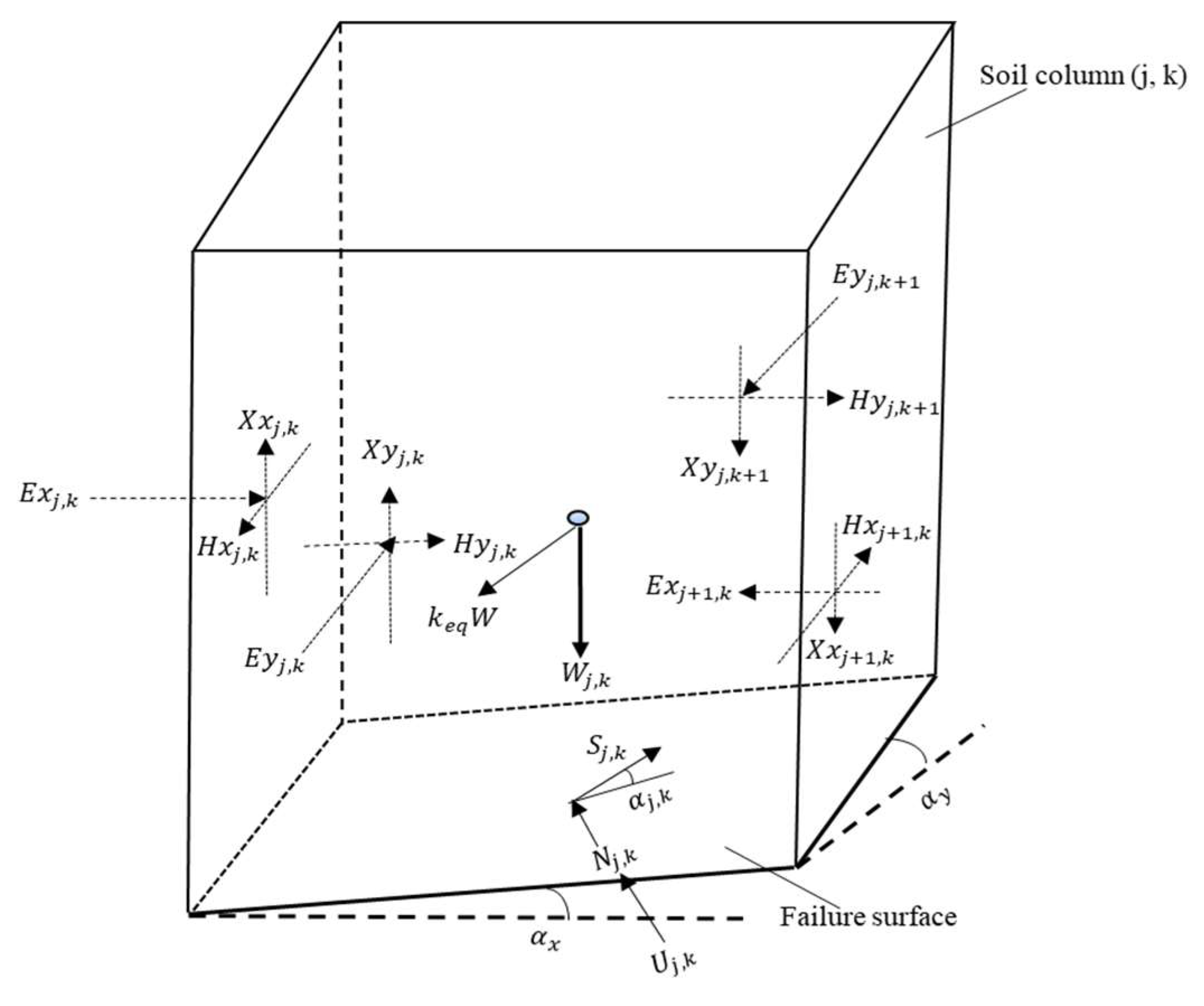
4.1. Deterministic Analysis
4.2. Digital Elevation Modelling
4.3. Probabilistic Analysis
5. Overview of Employed Models
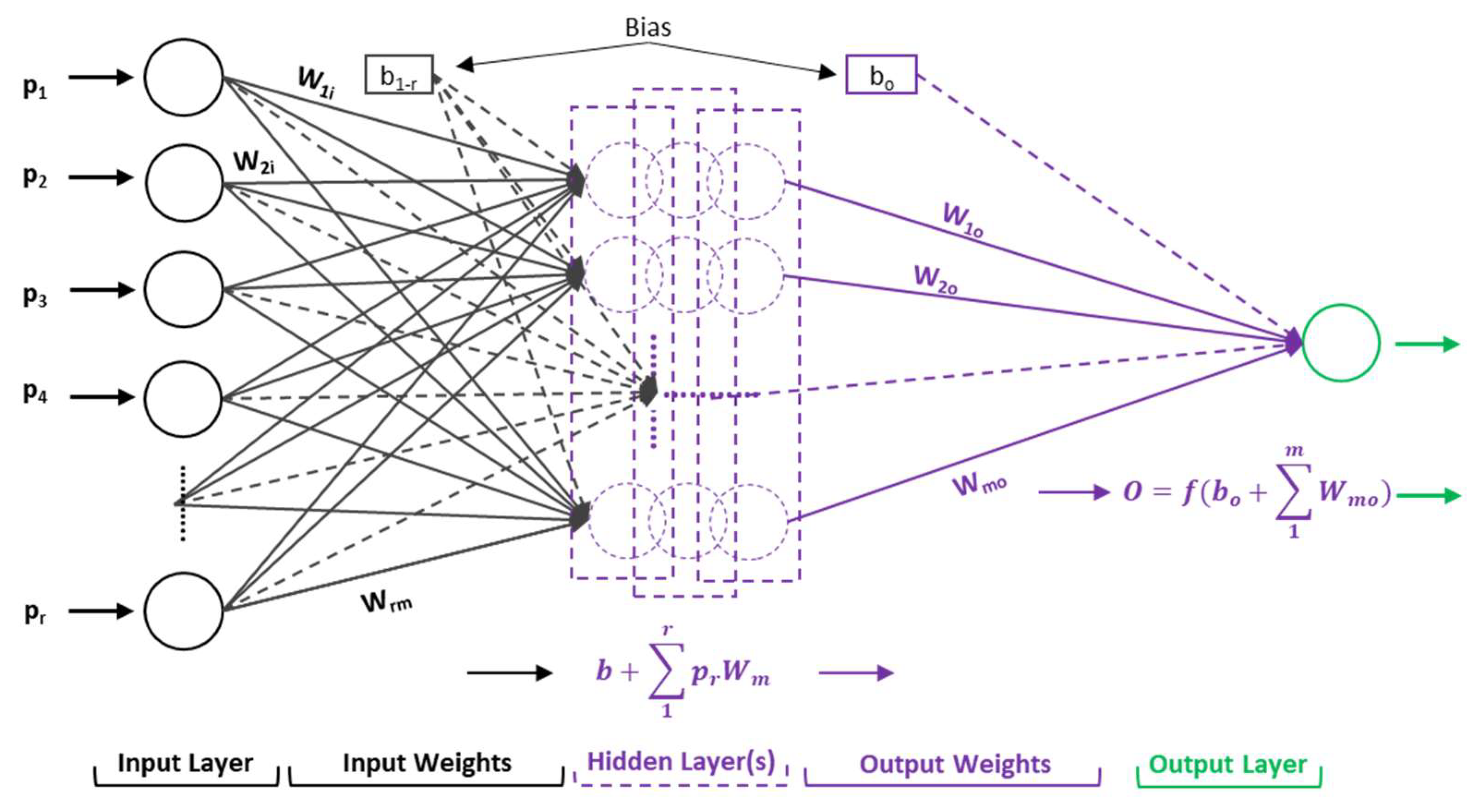
5.1. Artificial Neural Network
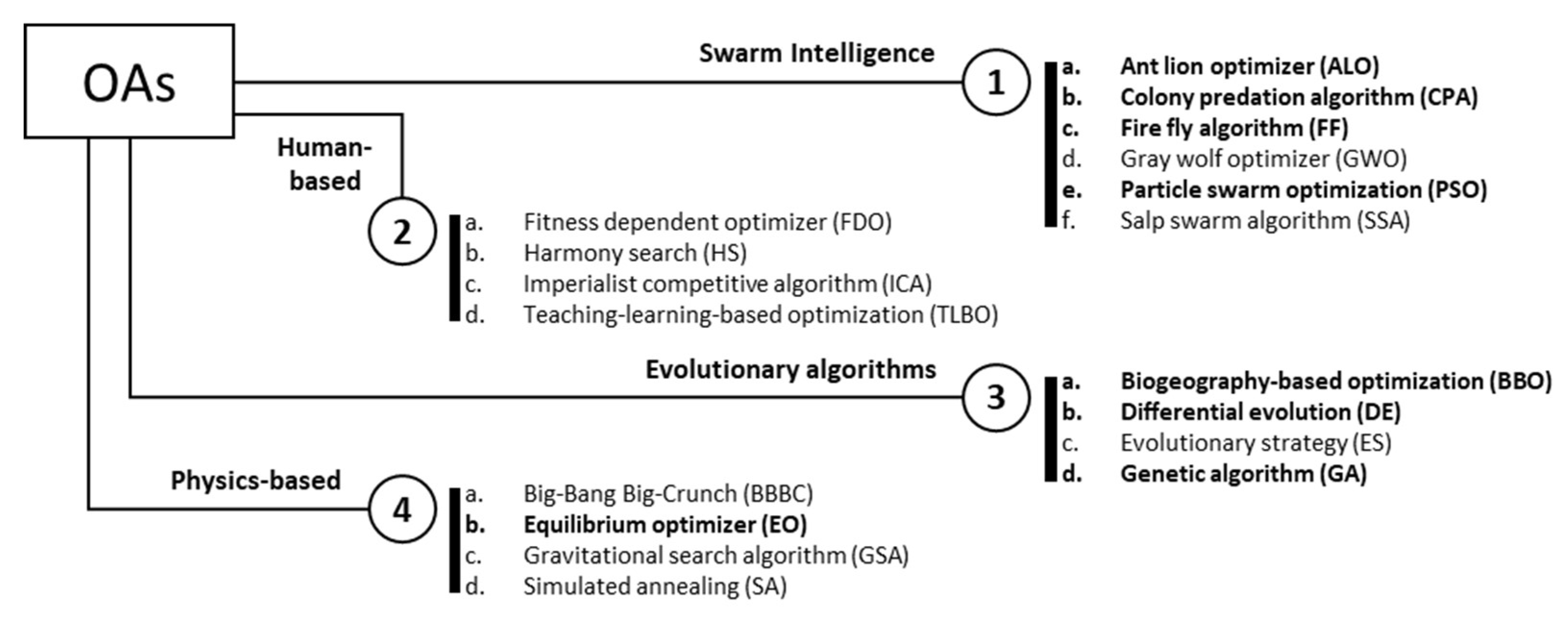
5.2. Overview of OAs
5.3. Hybridization Procedure of ANN and OAs
6. Data Description and Modelling
7. Results and Discussions
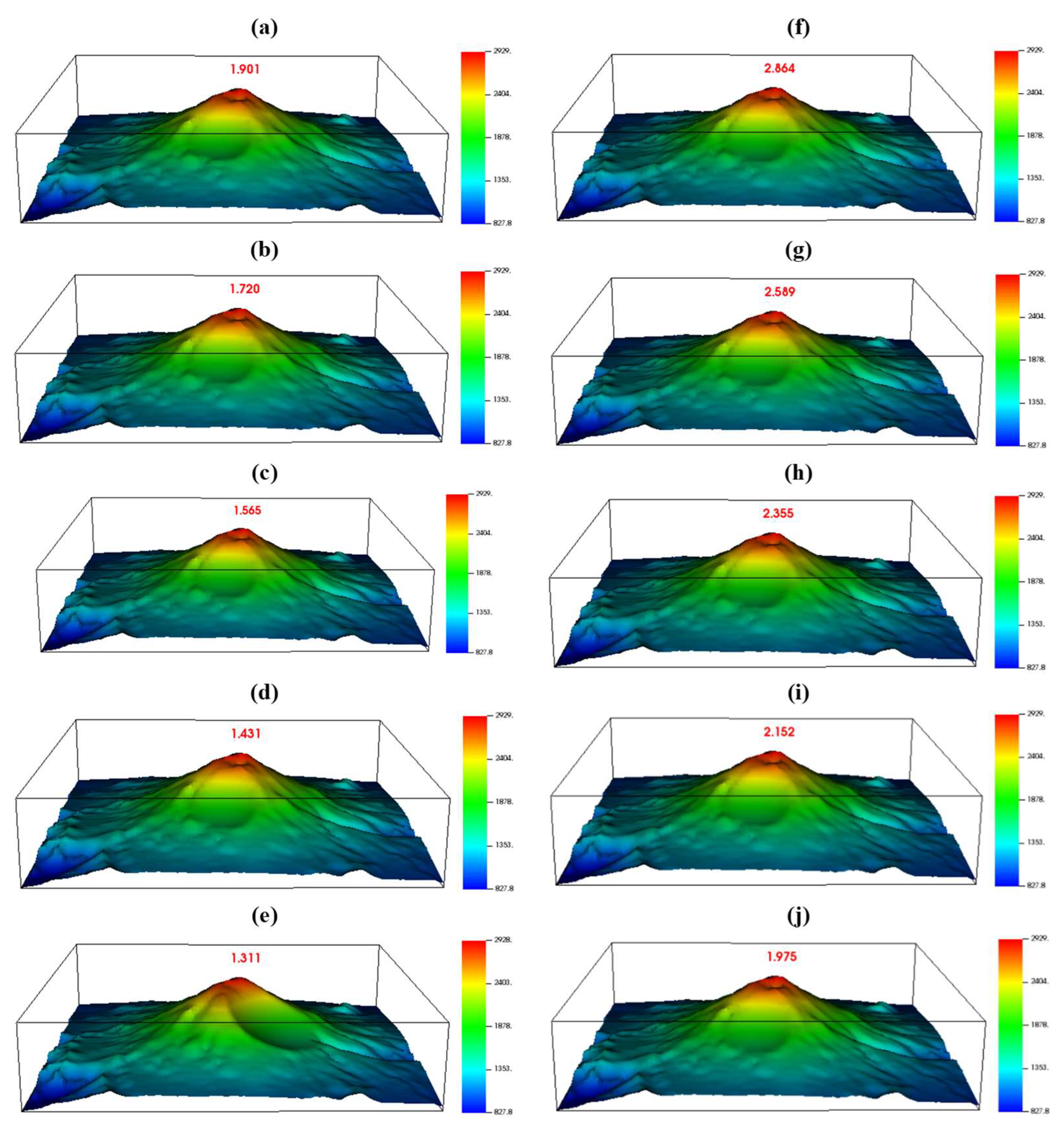
7.1. Slope Stability Analysis
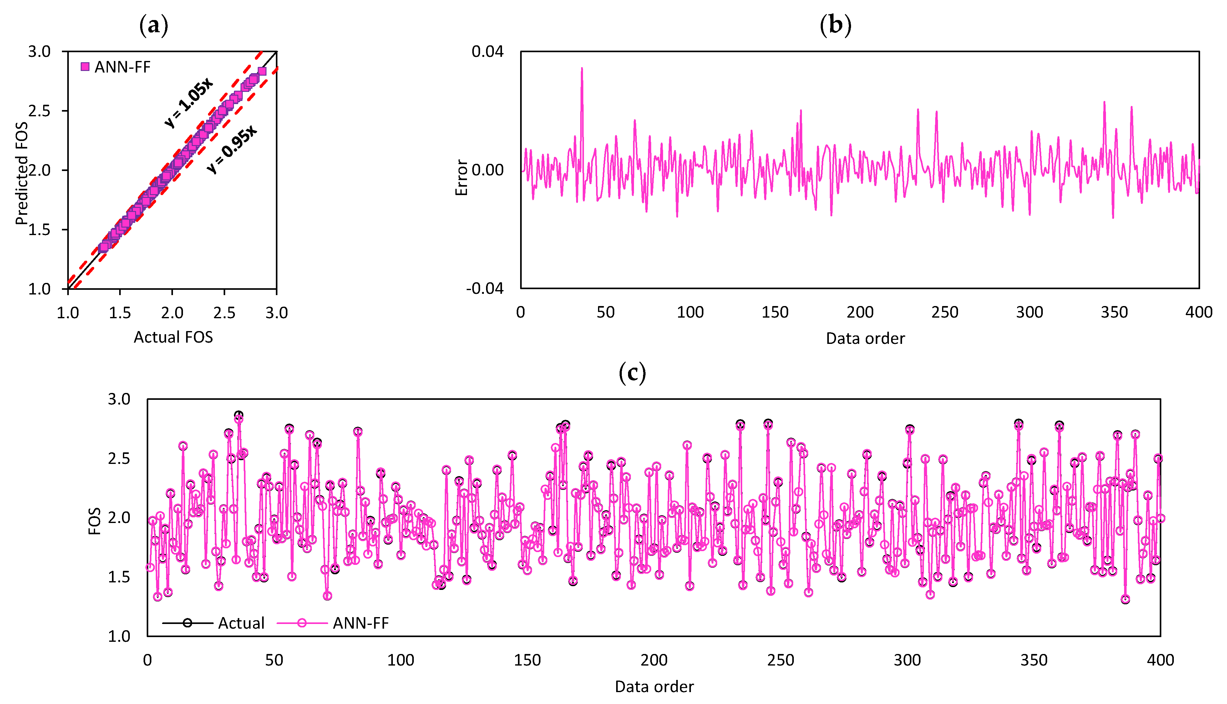
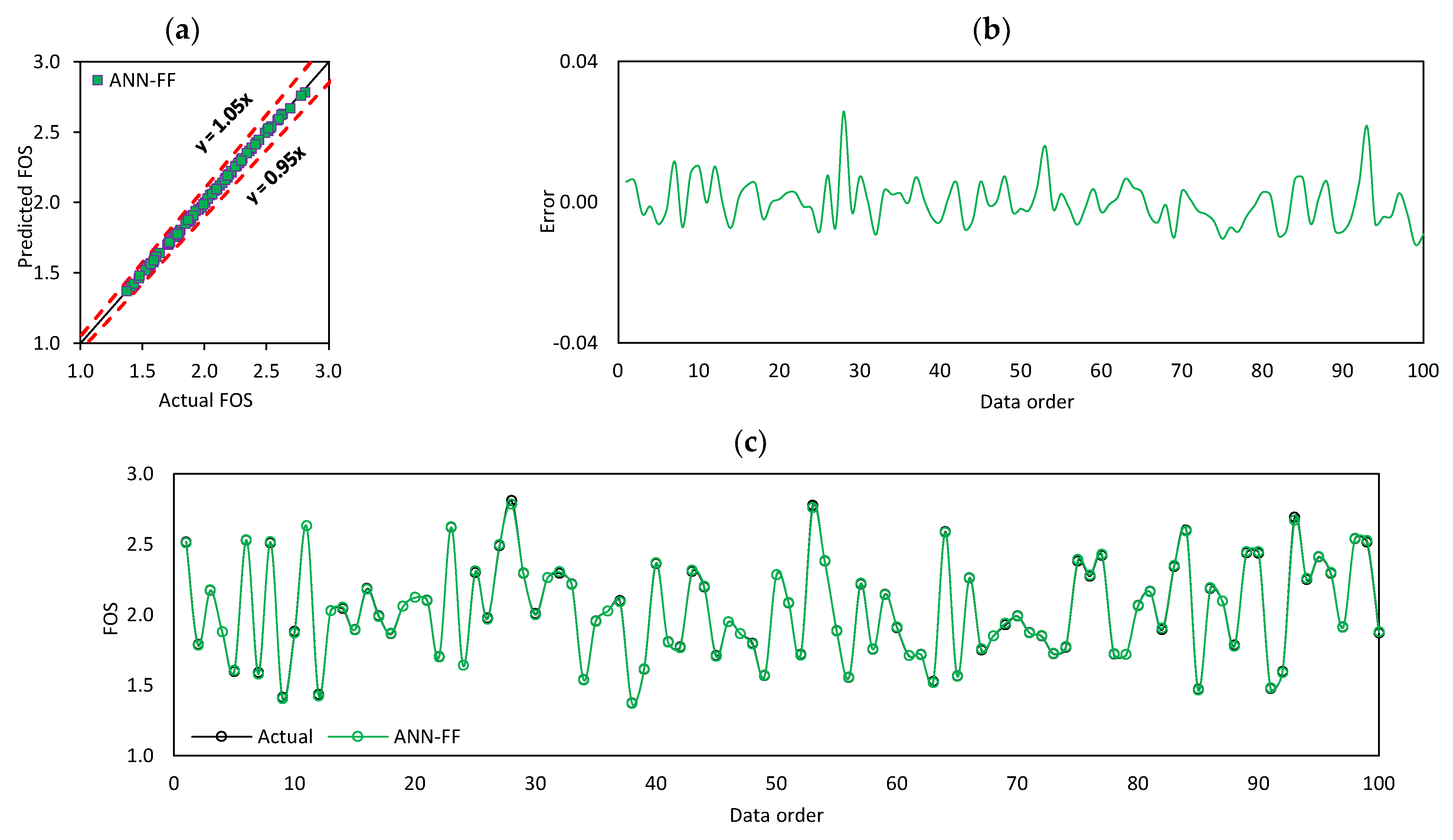
7.2. Computational Modelling and Performance Assessment
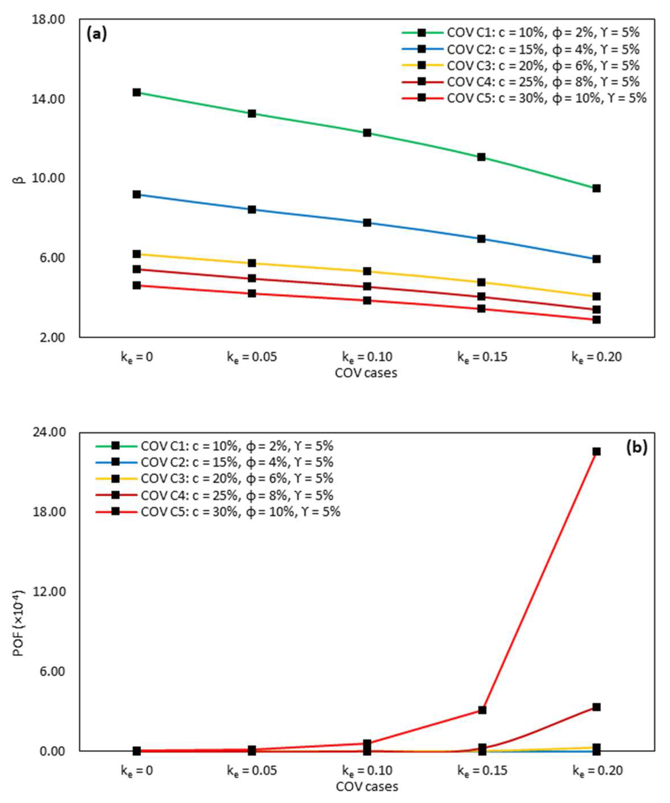
7.3. Assessment of POF
8. Summary and Conclusions
Supplementary Materials
Author Contributions
Funding
Data Availability Statement
Conflicts of Interest
Abbreviations
| 2D | Two-dimensional |
| 3D | Three-dimensional |
| ABC | Artificial bee colony |
| ALO | Ant lion optimizer |
| ANN | Artificial neural network |
| ANN-ABC | Hybrid model of ANN and ABC |
| ANN-ALO | Hybrid model of ANN and ALO |
| ANN-BBO | Hybrid model of ANN and BBO |
| ANN-CPA | Hybrid model of ANN and CPA |
| ANN-DE | Hybrid model of ANN and DE |
| ANN-EO | Hybrid model of ANN and EO |
| ANN-FF | Hybrid model of ANN and FF |
| ANN-GA | Hybrid model of ANN and GA |
| ANN-PSO | Hybrid model of ANN and PSO |
| BBBC | Big Bang Big Crunch |
| BBO | Biogeography based optimization |
| COV | Coefficient of variation |
| CPA | Colony predation algorithm |
| DE | Differential evolution |
| DEM | Digital elevation model |
| EA | Evolutionary algorithms |
| ELM | Extreme learning machine |
| EO | Equilibrium optimizer |
| ES | Evolution strategy |
| FDO | Fitness Dependent Optimizer |
| FF | Fire fly algorithm |
| FORM | First-order reliability method |
| FOS | Factor of safety |
| FOSM | First-order second-moment method |
| GA | Genetic algorithm |
| GIS | Geographic information system |
| GSA | Gravitational search algorithm |
| GWO | Grey wolf optimizer |
| HS | Harmony search |
| ICA | Imperialist competitive algorithm |
| LEM | Limit equilibrium method |
| MAE | Mean absolute error |
| MARS | Multivariate adaptive regression splines |
| MCS | Monte Carlo simulation |
| ML | Machine learning |
| NSE | Nash-Sutcliffe efficiency |
| OA | Optimization algorithm |
| PI | Performance index |
| POF | Probability of failure |
| PSO | Particle swarm optimization |
| R2 | Coefficient of determination |
| RA | Reliability analysis |
| RMSE | Root mean square error |
| RSM | Response surface method |
| RVM | Relevance vector machine |
| SA | Simulated annealing |
| SI | Swarm intelligence |
| SRM | Strength reduction method |
| SSA | Salp swarm algorithm |
| TLBO | Teaching learning-based optimization |
| USGS | United States Geological Survey |
| WMAPE | Weighted mean absolute percentage error |
| Nomenclature | |
| c | Cohesion |
| itrmax | maximum number of iterations |
| ke | seismic coefficient |
| lb | Lower bound |
| NHL | Number of hidden layers |
| NH | Number of hidden neurons |
| NS | Population/swarm size |
| ub | Upper bound |
| ϕ | Angle of internal friction |
| γ | Bulk density |
| β | Reliability index |
| μ | Mean |
| σ | Standard deviation |
| µFOS | Mean of FOS |
| σFOS | Standard deviation of FOS |
Appendix A. Sample Calculation

| FOS at ke = 0 | FOS at ke = 0.05 | FOS at ke = 0.10 | FOS at ke = 0.15 | FOS at ke = 0.20 | |||
|---|---|---|---|---|---|---|---|
| 1046.41 | 41.15 | 23.62 | 2.314 | 2.089 | 1.897 | 1.734 | 1.587 |
| 797.24 | 41.58 | 24.32 | 2.164 | 1.950 | 1.771 | 1.619 | 1.483 |
| 1049.63 | 40.14 | 23.84 | 2.248 | 2.030 | 1.846 | 1.687 | 1.542 |
| 1148.52 | 39.24 | 22.88 | 2.283 | 2.060 | 1.872 | 1.708 | 1.560 |
| 885.52 | 39.70 | 21.71 | 2.175 | 1.959 | 1.777 | 1.623 | 1.485 |
| 921.36 | 40.39 | 23.78 | 2.182 | 1.969 | 1.789 | 1.636 | 1.498 |
| 1038.03 | 40.56 | 23.88 | 2.265 | 2.045 | 1.859 | 1.699 | 1.554 |
| 940.10 | 38.51 | 25.82 | 2.034 | 1.842 | 1.682 | 1.540 | 1.407 |
| 1033.03 | 39.00 | 25.70 | 2.119 | 1.918 | 1.748 | 1.599 | 1.460 |
| 878.54 | 39.22 | 26.09 | 2.032 | 1.840 | 1.680 | 1.539 | 1.408 |
| 852.49 | 39.70 | 23.77 | 2.100 | 1.895 | 1.723 | 1.575 | 1.441 |
| 902.73 | 40.02 | 22.54 | 2.182 | 1.966 | 1.784 | 1.630 | 1.492 |
| 1015.86 | 41.65 | 22.80 | 2.347 | 2.118 | 1.922 | 1.757 | 1.609 |
| 998.84 | 40.78 | 22.61 | 2.288 | 2.064 | 1.873 | 1.712 | 1.567 |
| 942.17 | 39.21 | 25.13 | 2.091 | 1.891 | 1.724 | 1.577 | 1.443 |
| 977.59 | 39.21 | 24.06 | 2.141 | 1.934 | 1.760 | 1.610 | 1.472 |
| 1149.28 | 39.61 | 23.85 | 2.278 | 2.057 | 1.869 | 1.706 | 1.557 |
| 1170.86 | 39.69 | 25.78 | 2.237 | 2.021 | 1.838 | 1.676 | 1.527 |
| 865.25 | 40.80 | 22.80 | 2.197 | 1.979 | 1.795 | 1.640 | 1.501 |
| 1088.80 | 40.22 | 23.02 | 2.301 | 2.077 | 1.887 | 1.723 | 1.575 |
| 933.46 | 40.11 | 22.94 | 2.195 | 1.979 | 1.798 | 1.643 | 1.504 |
| 1064.66 | 40.38 | 24.35 | 2.258 | 2.040 | 1.855 | 1.695 | 1.549 |
| 932.30 | 38.96 | 24.87 | 2.078 | 1.879 | 1.712 | 1.567 | 1.433 |
| 1111.25 | 39.74 | 26.13 | 2.195 | 1.986 | 1.808 | 1.651 | 1.507 |
| 1010.37 | 39.19 | 25.14 | 2.131 | 1.928 | 1.756 | 1.606 | 1.468 |
| 1075.73 | 40.25 | 23.85 | 2.271 | 2.051 | 1.864 | 1.703 | 1.557 |
| 1112.64 | 40.15 | 24.03 | 2.283 | 2.062 | 1.874 | 1.711 | 1.563 |
| 998.55 | 41.15 | 25.07 | 2.242 | 2.026 | 1.843 | 1.686 | 1.543 |
| 921.31 | 40.47 | 22.52 | 2.221 | 2.001 | 1.816 | 1.659 | 1.519 |
| 1137.51 | 39.23 | 23.13 | 2.269 | 2.048 | 1.861 | 1.699 | 1.551 |
| μFOS | 2.204 | 1.990 | 1.809 | 1.654 | 1.512 | ||
| σFOS | 0.0842 | 0.0747 | 0.0659 | 0.0591 | 0.0539 | ||
| β | 14.30 | 13.26 | 12.28 | 11.06 | 9.51 | ||
| POF (%) | 1.1 × 10−44 | 2.1 × 10−38 | 5.5 × 10⁻³³ | 9.8 × 10⁻²⁷ | 9.7 × 10⁻²⁰ |
Appendix B. Details of Weights and Biases
| [1.2128 | 1.1998 | −0.0983 | 0.0943 | 0.4363 | −0.3550 | −0.4031 | −0.8791 |
| 1.7655 | 0.0843 | −0.4341 | 0.2536 | 2.1245 | −0.0737 | 1.6471 | −2.0288 |
| −0.3319 | 1.1062 | 0.0289 | −0.0084 | 0.4660 | −0.6024 | 1.3598 | 0.4425 |
| 0.9995 | 0.7243 | 0.4918 | −0.2207 | 0.1650 | −0.9283 | 0.2813 | −1.2230] |
| [−2.2941 | −1.3986 | 1.4235 | 0.0455 | 0.2659 | −0.8758 | −1.8870 | 2.4074] |
| [−0.0643 | −0.0304 | −1.1639 | 1.3973 | 0.0009 | 0.0614 | 0.0022 | −0.0685] |
| [0.7887] |
References
- Siebert, L. Large volcanic debris avalanches: Characteristics of source areas, deposits, and associated eruptions. J. Volcanol. Geotherm. Res. 1984, 22, 163–197. [Google Scholar] [CrossRef]
- Ui, T. Volcanic dry avalanche deposits—Identification and comparison with nonvolcanic debris stream deposits. J. Volcanol. Geotherm. Res. 1983, 18, 135–150. [Google Scholar] [CrossRef]
- Voight, B.; Elsworth, D. Failure of volcano slopes. Geotechnique 1997, 47, 1–31. [Google Scholar] [CrossRef]
- Voight, B.; Janda, R.J.; Glicken, H.; Douglass, P.M. Nature and mechanics of the Mount St Helens rockslide-avalanche of 18 May 1980. Geotechnique 1983, 33, 243–273. [Google Scholar] [CrossRef]
- Siebert, L.; Glicken, H.; Ui, T. Volcanic hazards from Bezymianny-and Bandai-type eruptions. Bull. Volcanol. 1987, 49, 435–459. [Google Scholar] [CrossRef]
- Reid, M.E. Transient thermal pressurization in hydrothermal systems: A cause of large-scale edifice collapse at volcanoes? Geol. Soc. Am. Abstr. Programs 1994, 26, A376. [Google Scholar]
- Bishop, A.W. The use of the slip circle in the stability analysis of slopes. Geotechnique 1955, 5, 7–17. [Google Scholar] [CrossRef]
- Zhang, Y.; Chen, G.; Zheng, L.; Li, Y.; Zhuang, X. Effects of geometries on three-dimensional slope stability. Can. Geotech. J. 2013, 50, 233–249. [Google Scholar] [CrossRef]
- Kalatehjari, R.; Arefnia, A.; Rashid, A.S.A.; Ali, N.; Hajihassani, M. Determination of Three-Dimensional Shape of Failure in Soil Slopes. Can. Geotech. J. 2015, 52, 1283–1301. [Google Scholar] [CrossRef]
- Hovland, H.J. Three-dimensional slope stability analysis method. J. Geotech. Eng. Div. 1977, 103, 971–986. [Google Scholar] [CrossRef]
- Xing, Z. Three-dimensional stability analysis of concave slopes in plan view. J. Geotech. Eng. 1988, 114, 658–671. [Google Scholar] [CrossRef]
- Sun, C.; Chai, J.; Xu, Z.; Qin, Y. 3D stability charts for convex and concave slopes in plan view with homogeneous soil based on the strength-reduction method. Int. J. Geomech. 2017, 17, 6016034. [Google Scholar] [CrossRef]
- Kumar, S.; Choudhary, S.S.; Burman, A. Recent advances in 3D slope stability analysis: A detailed review. Model. Earth Syst. Environ. 2022, 9, 1445–1462. [Google Scholar] [CrossRef]
- Hungr, O. An extension of Bishop’s simplified method of slope stability analysis to three dimensions. Geotechnique 1987, 37, 113–117. [Google Scholar] [CrossRef]
- Bishop, A.W. The analysis of stability of slopes. Géotechnique 1955, 5, 7. [Google Scholar] [CrossRef]
- Lam, L.; Fredlund, D. A general limit equilibrium model for three-dimensional slope stability analysis. Can. Geotech. J. 1993, 30, 905–919. [Google Scholar] [CrossRef]
- Fredlund, D.G.; Krahn, J. Comparison of slope stability methods of analysis. Can. Geotech. J. 1977, 14, 429–439. [Google Scholar] [CrossRef]
- An, Y.; Li, J.; Yue, J.; Zhou, J. Effect of seepage force on tunnel face stability using limit analysis with SRM. Geotech. Geol. Eng. 2021, 39, 1743–1751. [Google Scholar] [CrossRef]
- Liu, S.Y.; Shao, L.T.; Li, H.J. Slope stability analysis using the limit equilibrium method and two finite element methods. Comput. Geotech. 2015, 63, 291–298. [Google Scholar] [CrossRef]
- Zhao, H. Slope reliability analysis using a support vector machine. Comput. Geotech. 2008, 35, 459–467. [Google Scholar] [CrossRef]
- Safa, M.; Maleka, A.; Arjomand, M.A.; Khorami, M.; Shariati, M. Strain rate effects on soil-geosynthetic interaction in fine-grained soil. Geomech. Eng. 2019, 19, 533. [Google Scholar]
- Duncan, J.M. Factors of safety and reliability in geotechnical engineering. J. Geotech. Geoenviron. Eng. 2000, 126, 307–316. [Google Scholar] [CrossRef]
- Cao, Z.; Wang, Y.; Li, D. Probabilistic Approaches for Geotechnical Site Characterization and Slope Stability Analysis; Springer: Berlin/Heidelberg, Germany, 2017. [Google Scholar]
- Phoon, K.-K.; Ching, J. Risk and Reliability in Geotechnical Engineering; CRC Press: Boca Raton, FL, USA, 2015. [Google Scholar]
- Xie, M.; Esaki, T.; Zhou, G.; Mitani, Y. Three-dimensional stability evaluation of landslides and a sliding process simulation using a new geographic information systems component. Environ. Geol. 2003, 43, 503–512. [Google Scholar] [CrossRef]
- Wong, F.S. Slope reliability and response surface method. J. Geotech. Eng. 1985, 111, 32–53. [Google Scholar] [CrossRef]
- Zhao, H.; Yin, S.; Ru, Z. Relevance vector machine applied to slope stability analysis. Int. J. Numer. Anal. Methods Géoméch. 2012, 36, 643–652. [Google Scholar] [CrossRef]
- Bardhan, A.; Samui, P. Probabilistic slope stability analysis of Heavy-haul freight corridor using a hybrid machine learning paradigm. Transp. Geotech. 2022, 37, 100815. [Google Scholar] [CrossRef]
- Deng, J. Structural reliability analysis for implicit performance function using radial basis function network. Int. J. Solids Struct. 2006, 43, 3255–3291. [Google Scholar] [CrossRef]
- Deng, J.; Gu, D.; Li, X.; Yue, Z.Q. Structural reliability analysis for implicit performance functions using artificial neural network. Struct. Saf. 2005, 27, 25–48. [Google Scholar] [CrossRef]
- Cho, S.E. Probabilistic stability analyses of slopes using the ANN-based response surface. Comput. Geotech. 2009, 36, 787–797. [Google Scholar] [CrossRef]
- Erzin, Y.; Cetin, T. The use of neural networks for the prediction of the critical factor of safety of an artificial slope subjected to earthquake forces. Sci. Iran. 2012, 19, 188–194. [Google Scholar] [CrossRef]
- Kang, F.; Xu, Q.; Li, J. Slope reliability analysis using surrogate models via new support vector machines with swarm intelligence. Appl. Math. Model. 2016, 40, 6105–6120. [Google Scholar] [CrossRef]
- Li, S.; Zhao, H.; Ru, Z. Relevance vector machine-based response surface for slope reliability analysis. Int. J. Numer. Anal. Methods Géoméch. 2017, 41, 1332–1346. [Google Scholar] [CrossRef]
- Chen, J.; Wen, L.; Bi, C.; Liu, Z.; Liu, X.; Yin, L.; Zheng, W. Multifractal analysis of temporal and spatial characteristics of earthquakes in Eurasian seismic belt. Open Geosci. 2023, 15, 20220482. [Google Scholar] [CrossRef]
- Reid, M.E.; Christian, S.B.; Brien, D.L.; Henderson, S. Scoops3D—Software to analyze three-dimensional slope stability throughout a digital landscape. In U.S. Geological Survey Techniques and Methods; U.S. Geological Survey: Reston, VA, USA, 2015. [Google Scholar]
- Le, L.T.; Nguyen, H.; Dou, J.; Zhou, J. A comparative study of PSO-ANN, GA-ANN, ICA-ANN, and ABC-ANN in estimating the heating load of buildings’ energy efficiency for smart city planning. Appl. Sci. 2019, 9, 2630. [Google Scholar] [CrossRef]
- Tun, Y.W.; Llano-Serna, M.A.; Pedroso, D.M.; Scheuermann, A. Multimodal reliability analysis of 3D slopes with a genetic algorithm. Acta Geotech. 2019, 14, 207–223. [Google Scholar] [CrossRef]
- Glicken, H. Rockslide-Debris Avalanche of May 18, 1980, Mount St. Helens Volcano, Washington; U.S. Geological Survey, Cascades Volcano Observatory: Reston, VA, USA, 1996. [Google Scholar]
- Hopson, C.A.; Melson, W.G. Stratigraphy of Mount St. Helens 1980 crater walls. EOS. Trans. Am. Geophys. Union 1982, 63, 13. [Google Scholar]
- Balasubramanian, A. Digital Elevation Model (DEM) in GIS; University of Mysore: Mysuru, India, 2017. [Google Scholar]
- Xu, Y.; Zhao, M.-W.; Lu, J.; Wang, C.; Jiang, L.; Yang, C.-C.; Huang, X.-L. Methods for the construction of DEMs of artificial slopes considering morphological features and semantic information. J. Mt. Sci. 2022, 19, 563–577. [Google Scholar] [CrossRef]
- Wise, S. Assessing the quality for hydrological applications of digital elevation models derived from contours. Hydrol. Process. 2000, 14, 1909–1929. [Google Scholar] [CrossRef]
- Zhou, G.; Zhou, X.; Song, Y.; Xie, D.; Wang, L.; Yan, G.; Hu, M.; Liu, B.; Shang, W.; Gong, C.; et al. Design of supercontinuum laser hyperspectral light detection and ranging (LiDAR)(SCLaHS LiDAR). Int. J. Remote Sens. 2021, 42, 3731–3755. [Google Scholar] [CrossRef]
- Zhou, G.; Li, W.; Zhou, X.; Tan, Y.; Lin, G.; Li, X.; Deng, R. An innovative echo detection system with STM32 gated and PMT adjustable gain for airborne LiDAR. Int. J. Remote Sens. 2021, 42, 9187–9211. [Google Scholar] [CrossRef]
- Zhou, G.; Deng, R.; Zhou, X.; Long, S.; Li, W.; Lin, G.; Li, X. Gaussian inflection point selection for LiDAR hidden echo signal decomposition. IEEE Geosci. Remote Sens. Lett. 2021, 19, 1–5. [Google Scholar] [CrossRef]
- Zhou, G.; Yang, Z. Analysis for 3-D morphology structural changes for underwater topographical in Culebrita Island. Int. J. Remote Sens. 2023, 44, 2458–2479. [Google Scholar] [CrossRef]
- Zhuo, Z.; Du, L.; Lu, X.; Chen, J.; Cao, Z. Smoothed Lv distribution based three-dimensional imaging for spinning space debris. IEEE Trans. Geosci. Remote Sens. 2022, 60, 1–13. [Google Scholar] [CrossRef]
- Liu, Z.; Xu, J.; Liu, M.; Yin, Z.; Liu, X.; Yin, L.; Zheng, W. Remote sensing and geostatistics in urban water-resource monitoring: A review. Mar. Freshw. Res. 2023, 74, 747–765. [Google Scholar] [CrossRef]
- Cavazzi, S.; Corstanje, R.; Mayr, T.; Hannam, J.; Fealy, R. Are fine resolution digital elevation models always the best choice in digital soil mapping? Geoderma 2013, 195, 111–121. [Google Scholar] [CrossRef]
- Golafshani, E.M.; Behnood, A.; Arashpour, M. Predicting the compressive strength of normal and High-Performance Concretes using ANN and ANFIS hybridized with Grey Wolf Optimizer. Constr. Build. Mater. 2020, 232, 117266. [Google Scholar] [CrossRef]
- Apostolopoulou, M.; Asteris, P.G.; Armaghani, D.J.; Douvika, M.G.; Lourenço, P.B.; Cavaleri, L.; Bakolas, A.; Moropoulou, A. Mapping and holistic design of natural hydraulic lime mortars. Cem. Concr. Res. 2020, 136, 106167. [Google Scholar] [CrossRef]
- Asteris, P.G.; Kokoris, S.; Gavriilaki, E.; Tsoukalas, M.Z.; Houpas, P.; Paneta, M.; Koutzas, A.; Argyropoulos, T.; Alkayem, N.F.; Armaghani, D.J.; et al. Early prediction of COVID-19 outcome using artificial intelligence techniques and only five laboratory indices. Clin. Immunol. 2023, 246, 109218. [Google Scholar] [CrossRef]
- Asteris, P.G.; Gavriilaki, E.; Touloumenidou, T.; Koravou, E.; Koutra, M.; Papayanni, P.G.; Pouleres, A.; Karali, V.; Lemonis, M.E.; Mamou, A.; et al. Genetic prediction of icu hospitalization and mortality in COVID-19 patients using artificial neural networks. J. Cell. Mol. Med. 2022, 26, 1445–1455. [Google Scholar] [CrossRef]
- Asteris, P.G.; Armaghani, D.J.; Hatzigeorgiou, G.D.; Karayannis, C.G.; Pilakoutas, K. Predicting the shear strength of reinforced concrete beams using Artificial Neural Networks. Comput. Concr. An. Int. J. 2019, 24, 469–488. [Google Scholar]
- Elaziz, M.A.; Dahou, A.; Abualigah, L.; Yu, L.; Alshinwan, M.; Khasawneh, A.M.; Lu, S. Advanced metaheuristic optimization techniques in applications of deep neural networks: A review. Neural Comput. Appl. 2021, 33, 14079–14099. [Google Scholar] [CrossRef]
- Seyedali, M. The ant lion optimizer. Adv. Eng. Softw. 2015, 83, 80–98. [Google Scholar]
- Tu, J.; Chen, H.; Wang, M.; Gandomi, A.H. The colony predation algorithm. J. Bionic Eng. 2021, 18, 674–710. [Google Scholar] [CrossRef]
- Yang, X.S.; He, X. Firefly algorithm: Recent advances and applications. Int. J. Swarm Intell. 2013, 1, 36–50. [Google Scholar] [CrossRef]
- Mirjalili, S.; Mirjalili, S.M.; Lewis, A. Grey Wolf Optimizer. Adv. Eng. Softw. 2014, 69, 46–61. [Google Scholar] [CrossRef]
- Kennedy, J.; Eberhart, R. Particle swarm optimization. In Proceedings of the ICNN’95—International Conference on Neural Networks, Perth, WA, Australia, 27 November 1995–1 December 1995; IEEE: Piscataway, NJ, USA, 1995; Volume 4, pp. 1942–1948. [Google Scholar]
- Abualigah, L.; Shehab, M.; Alshinwan, M.; Alabool, H. Salp swarm algorithm: A comprehensive survey. Neural Comput. Appl. 2020, 32, 11195–11215. [Google Scholar] [CrossRef]
- Abdullah, J.M.; Ahmed, T. Fitness dependent optimizer: Inspired by the bee swarming reproductive process. IEEE Access 2019, 7, 43473–43486. [Google Scholar] [CrossRef]
- Geem, Z.W.; Kim, J.H.; Loganathan, G.V. A new heuristic optimization algorithm: Harmony search. Simulation 2001, 76, 60–68. [Google Scholar] [CrossRef]
- Atashpaz-Gargari, E.; Lucas, C. Imperialist competitive algorithm: An algorithm for optimization inspired by imperialistic competition. In Proceedings of the 2007 IEEE Congress on Evolutionary Computation, Singapore, 25–28 September 2007; IEEE: Piscataway, NJ, USA, 2007; pp. 4661–4667. [Google Scholar]
- Rao, R.V.; Savsani, V.J.; Vakharia, D.P. Teaching–learning-based optimization: A novel method for constrained mechanical design optimization problems. Comput. Aided Des. 2011, 43, 303–315. [Google Scholar] [CrossRef]
- Simon, D. Biogeography-based optimization. IEEE Trans. Evol. Comput. 2008, 12, 702–713. [Google Scholar] [CrossRef]
- Storn, R.; Price, K. Differential evolution-a simple and efficient heuristic for global optimization over continuous spaces. J. Glob. Optim. 1997, 11, 341. [Google Scholar] [CrossRef]
- Rechenberg, I. Evolution strategy: Nature’s way of optimization. In Optimization: Methods and Applications, Possibilities and Limitations: Proceedings of an International Seminar Organized by Deutsche Forschungsanstalt für Luft-und Raumfahrt (DLR), Bonn, June; Springer: Berlin/Heidelberg, Germany, 1989; pp. 106–126. [Google Scholar]
- Goldberg, D.E.; Holland, J.H. Genetic Algorithms and Machine Learning. Mach. Learn. 1988, 3, 95–99. [Google Scholar] [CrossRef]
- Erol, O.K.; Eksin, I. A new optimization method: Big bang–big crunch. Adv. Eng. Softw. 2006, 37, 106–111. [Google Scholar] [CrossRef]
- Faramarzi, A.; Heidarinejad, M.; Stephens, B.; Mirjalili, S. Equilibrium optimizer: A novel optimization algorithm. Knowl.-Based Syst. 2020, 191, 105190. [Google Scholar] [CrossRef]
- Rashedi, E.; Nezamabadi-Pour, H.; Saryazdi, S. GSA: A gravitational search algorithm. Inf. Sci. 2009, 179, 2232–2248. [Google Scholar] [CrossRef]
- Kirkpatrick, S. Optimization by simulated annealing: Quantitative studies. J. Stat. Phys. 1984, 34, 975–986. [Google Scholar] [CrossRef]
- Koopialipoor, M.; Fallah, A.; Armaghani, D.J.; Azizi, A.; Mohamad, E.T. Three hybrid intelligent models in estimating flyrock distance resulting from blasting. Eng. Comput. 2019, 35, 243–256. [Google Scholar] [CrossRef]
- Chen, D.; Wang, Q.; Li, Y.; Li, Y.; Zhou, H.; Fan, Y. A general linear free energy relationship for predicting partition coefficients of neutral organic compounds. Chemosphere 2020, 247, 125869. [Google Scholar] [CrossRef]
- Wu, Z.; Huang, B.; Fan, J.; Chen, H. Homotopy based stochastic finite element model updating with correlated static measurement data. Measurement 2023, 210, 112512. [Google Scholar] [CrossRef]
- Harr, M.E. The Civil Engineering Handbook; CRC Press: Boca Raton, FL, USA, 2002; Chapter 18. [Google Scholar]


| Index | c (kN/m2) | ϕ (°) | γ (kN/m3) | ke |
|---|---|---|---|---|
| Min. | 809.77 | 35.18 | 22.02 | 0.00 |
| Mean | 1000.00 | 40.00 | 24.00 | - |
| Max. | 1195.17 | 49.40 | 25.99 | 0.20 |
| Stnd. Dev. | 117.31 | 4.21 | 1.17 | 0.08 |
| Stnd. Error | 11.73 | 0.04 | 0.01 | 0.02 |
| Kurtosis | −1.26 | −1.20 | −1.25 | −1.20 |
| Skewness | −0.08 | −0.09 | 0.16 | 0.00 |
| Indices | ANN-ALO | ANN-BBO | ANN-CPA | ANN-DE | ANN-EO | ANN-FF | ANN-GA | ANN-PSO | ANN |
|---|---|---|---|---|---|---|---|---|---|
| MAE | 0.0087 | 0.0128 | 0.0088 | 0.0520 | 0.0067 | 0.0031 | 0.0306 | 0.0212 | 0.0124 |
| NS | 0.9968 | 0.9933 | 0.9970 | 0.9024 | 0.9981 | 0.9996 | 0.9687 | 0.9826 | 0.9949 |
| PI | 1.9814 | 1.9691 | 1.9824 | 1.7385 | 1.9868 | 1.9952 | 1.8994 | 1.9367 | 1.9738 |
| R2 | 0.9968 | 0.9934 | 0.9970 | 0.9039 | 0.9981 | 0.9996 | 0.9688 | 0.9826 | 0.9950 |
| RMSE | 0.0121 | 0.0175 | 0.0117 | 0.0669 | 0.0094 | 0.0041 | 0.0378 | 0.0283 | 0.0159 |
| WMAPE | 0.0202 | 0.0295 | 0.0204 | 0.1206 | 0.0155 | 0.0072 | 0.0710 | 0.0490 | 0.0266 |
| Indices | ANN-ALO | ANN-BBO | ANN-CPA | ANN-DE | ANN-EO | ANN-FF | ANN-GA | ANN-PSO | ANN |
|---|---|---|---|---|---|---|---|---|---|
| MAE | 0.0095 | 0.0144 | 0.0102 | 0.0555 | 0.0078 | 0.0032 | 0.0342 | 0.0255 | 0.0102 |
| NS | 0.9969 | 0.9927 | 0.9963 | 0.8938 | 0.9978 | 0.9996 | 0.9551 | 0.9722 | 0.9961 |
| PI | 1.9813 | 1.9667 | 1.9791 | 1.7112 | 1.9853 | 1.9951 | 1.8634 | 1.9074 | 1.9789 |
| R2 | 0.9969 | 0.9931 | 0.9964 | 0.8939 | 0.9979 | 0.9996 | 0.9563 | 0.9727 | 0.9961 |
| RMSE | 0.0124 | 0.0188 | 0.0135 | 0.0721 | 0.0103 | 0.0042 | 0.0469 | 0.0369 | 0.0133 |
| WMAPE | 0.0206 | 0.0311 | 0.0220 | 0.1198 | 0.0169 | 0.0070 | 0.0737 | 0.0549 | 0.0233 |
| Parameter | Mean | COV (%) Cases | COV | Reference | ||||
|---|---|---|---|---|---|---|---|---|
| Case 1 | Case 2 | Case 3 | Case 4 | Case 5 | Value/Range | |||
| c | 1000 | 10% | 15% | 20% | 25% | 30% | 23% | Tun et al. [38] |
| ϕ | 40 | 2% | 4% | 6% | 8% | 10% | 7% | Tun et al. [38] |
| γ | 24 | 5% | 5% | 5% | 5% | 5% | 3–7% | Harr [78] |
| Cases | β and POF | β and POF (%) | ||||
|---|---|---|---|---|---|---|
| Set 1 | Set 2 | Set 3 | Set 4 | Set 5 | ||
| Case 1 | β | 14.30 | 13.26 | 12.33 | 11.06 | 9.51 |
| POF | 1.1 × 10−44 | 2.1 × 10−38 | 5.5 × 10⁻³³ | 9.8 × 10⁻²⁷ | 9.7 × 10⁻²⁰ | |
| Case 2 | β | 9.17 | 8.43 | 7.97 | 6.97 | 5.96 |
| POF | 2.4 × 10⁻¹⁸ | 1.7 × 10⁻¹⁵ | 3.9 × 10⁻¹³ | 1.6 × 10⁻¹⁰ | 1.3 × 10⁻⁷ | |
| Case 3 | β | 6.17 | 5.72 | 5.28 | 4.77 | 4.06 |
| POF | 3.3 × 10⁻⁸ | 5.4 × 10⁻⁷ | 5.4 × 10⁻⁶ | 9.2 × 10⁻⁵ | 2.5 × 10⁻³ | |
| Case 4 | β | 5.45 | 4.98 | 4.67 | 4.07 | 3.42 |
| POF | 2.5 × 10⁻⁶ | 3.2 × 10⁻⁵ | 2.4 × 10⁻⁴ | 2.4 × 10⁻³ | 3.1 × 10⁻² | |
| Case 5 | β | 4.64 | 4.23 | 3.63 | 3.44 | 2.89 |
| POF | 1.7 × 10⁻⁴ | 1.2 × 10⁻³ | 0.01 | 0.03 | 0.19 | |
Disclaimer/Publisher’s Note: The statements, opinions and data contained in all publications are solely those of the individual author(s) and contributor(s) and not of MDPI and/or the editor(s). MDPI and/or the editor(s) disclaim responsibility for any injury to people or property resulting from any ideas, methods, instructions or products referred to in the content. |
© 2023 by the authors. Licensee MDPI, Basel, Switzerland. This article is an open access article distributed under the terms and conditions of the Creative Commons Attribution (CC BY) license (https://creativecommons.org/licenses/by/4.0/).
Share and Cite
Kumar, S.; Choudhary, S.S.; Burman, A.; Singh, R.K.; Bardhan, A.; Asteris, P.G. Probabilistic Slope Stability Analysis of Mount St. Helens Using Scoops3D and a Hybrid Intelligence Paradigm. Mathematics 2023, 11, 3809. https://doi.org/10.3390/math11183809
Kumar S, Choudhary SS, Burman A, Singh RK, Bardhan A, Asteris PG. Probabilistic Slope Stability Analysis of Mount St. Helens Using Scoops3D and a Hybrid Intelligence Paradigm. Mathematics. 2023; 11(18):3809. https://doi.org/10.3390/math11183809
Chicago/Turabian StyleKumar, Sumit, Shiva Shankar Choudhary, Avijit Burman, Raushan Kumar Singh, Abidhan Bardhan, and Panagiotis G. Asteris. 2023. "Probabilistic Slope Stability Analysis of Mount St. Helens Using Scoops3D and a Hybrid Intelligence Paradigm" Mathematics 11, no. 18: 3809. https://doi.org/10.3390/math11183809
APA StyleKumar, S., Choudhary, S. S., Burman, A., Singh, R. K., Bardhan, A., & Asteris, P. G. (2023). Probabilistic Slope Stability Analysis of Mount St. Helens Using Scoops3D and a Hybrid Intelligence Paradigm. Mathematics, 11(18), 3809. https://doi.org/10.3390/math11183809