Generalized Penalized Constrained Regression: Sharp Guarantees in High Dimensions with Noisy Features

Abstract

The generalized penalized constrained regression (G-PCR) is a penalized model for high-dimensional linear inverse problems with structured features. This paper presents a sharp error performance analysis of the G-PCR in the over-parameterized high-dimensional setting. The analysis is carried out under the assumption of a noisy or erroneous Gaussian features matrix. To assess the performance of the G-PCR problem, the study employs multiple metrics such as prediction risk, cosine similarity, and the probabilities of misdetection and false alarm. These metrics offer valuable insights into the accuracy and reliability of the G-PCR model under different circumstances. Furthermore, the derived results are specialized and applied to well-known instances of G-PCR, including ${\mathcal{l}}_1$-norm penalized regression for sparse signal recovery and ${\mathcal{l}}_2$-norm (ridge) penalization. These specific instances are widely utilized in regression analysis for purposes such as feature selection and model regularization. To validate the obtained results, the paper provides numerical simulations conducted on both real-world and synthetic datasets. Using extensive simulations, we show the universality and robustness of the results of this work to the assumed Gaussian distribution of the features matrix. We empirically investigate the so-called double descent phenomenon and show how optimal selection of the hyper-parameters of the G-PCR can help mitigate this phenomenon. The derived expressions and insights from this study can be utilized to optimally select the hyper-parameters of the G-PCR. By leveraging these findings, one can make well-informed decisions regarding the configuration and fine-tuning of the G-PCR model, taking into consideration the specific problem at hand as well as the presence of noisy features in the high-dimensional setting.

1. Introduction

1.1. Notations and Definitions

To avoid confusion, we start by introducing the notations and definitions used throughout this paper. For any positive integer p, let $\left[p\right]$ denote the set $\{1,2,\cdots ,p\}$. Bold face lower case letters (e.g., θ) represent a column vector, and ${\theta }_i$ is its ith entry, while ${\parallel \mathit{\theta }\parallel }_q={\left({\sum }_{i=1}^p{\left|{\theta }_i\right|}^q\right)}^{\frac{1}{q}}$ is its ${\mathcal{l}}_q$-norm. The ${\mathcal{l}}_{\infty }$-norm of a vector is defined as: ${\parallel \mathit{\theta }\parallel }_{\infty }$$={max}_i\left|{\theta }_i\right|$. Upper case bold letters such as X are used to indicate matrices, with ${\mathbf{I}}_p$ representing the $p\times p$ identity matrix. The symbols ${(·)}^{-1}$ and ${(·)}^{\top }$ are the inversion and transpose operations, respectively. We use $\mathbb{P}(·)$ and $\mathbb{E}[·]$ to indicate the probability of an event and the expected value of a random variable, respectively. The notation $“\stackrel{P}{⟶}”$ is used to represent convergence in probability. We write $X\sim p_X$ to indicate that a random variable X is randomly distributed according to a probability mass (or density) function $p_X$. Particularly, $\mathbf{v}\sim \mathsf{N}(\mathbf{0},{\mathbf{C}}_{\mathbf{v}})$ means that the random vector v has a normal distribution with $\mathbf{0}$ mean vector and covariance matrix ${\mathbf{C}}_{\mathbf{v}}=\mathbb{E}\left[\mathbf{v}{\mathbf{v}}^{\top }\right]$, where $\mathbf{0}$ is the zero vector. For $m\in \mathbb{N}$, a function $\psi :{\mathbb{R}}^m\to \mathbb{R}$ is said to be pseudo-Lipschitz of order $k\ge 1$ if there exists a constant $L>0$ such that, for all, $\mathit{x},\mathbf{y}\in {\mathbb{R}}^m$: $\left|\psi \left(\mathit{x}\right)-\psi \left(\mathbf{y}\right)\right|\le {L(1+\parallel \mathit{x}\parallel }_2^{k-1}+{\parallel \mathbf{y}\parallel }_2^{k-1}{)\parallel \mathit{x}-\mathbf{y}\parallel }_2$.

A function $\mathcal{P}:{\mathbb{R}}^p\to \mathbb{R}$ is called separable if $\mathcal{P}\left(\mathit{x}\right)={\sum }_{j=1}^p\tilde{\mathcal{P}}\left(x_j\right)\forall \mathit{x}\in {\mathbb{R}}^p$, where $\tilde{\mathcal{P}}:\mathbb{R}\to \mathbb{R}$ is a real-valued function. The notation ${\mathbf{1}}_{\left\{\mathcal{A}\right\}}$ is the indicator function, which is defined as

$${\mathbf{1}}_{\left\{\mathcal{A}\right\}}\left(x\right)=\left\{\begin{array}{cc}1,\hfill & \mathrm{if}x\in \mathcal{A},\hfill \\ 0,\hfill & \mathrm{otherwise}.\hfill \end{array}\right.$$

Finally, we need the following definitions:

• The generalized Moreau envelope function of a proper convex function $h:\mathbb{R}\to \mathbb{R}$ is defined as

  $${\mathsf{M}}_h(a;b,c,d)=\underset{c\le x\le d}{min}\frac{1}{2}{(x-a)}^2+bh\left(x\right)$$

  (1)

  for $a,b,c,d\in \mathbb{R}$, with $b\ge 0, c\le 0$ and $d\ge 0$. The generalized Moreau envelope given above is an extended version of the well-known Moreau–Yosida envelope function [1].
• The minimizer of the above function is called the generalized proximal operator, which is given as

  $${\mathrm{prox}}_h(a;b,c,d)=\arg \underset{c\le x\le d}{min}\frac{1}{2}{(x-a)}^2+bh\left(x\right).$$

1.2. Motivation

Suppose we observe a response vector y $\in {\mathbb{R}}^n$ and a data matrix X $\in {\mathbb{R}}^{n\times p}$ according to the linear model

$$\mathbf{y}=\mathbf{X}{\mathit{\theta }}_0+\mathit{ϵ},$$

(2)

where ${\mathit{\theta }}_0\in {\mathbb{R}}^p$ is a vector of coefficients or parameters, or an unknown signal vector, and $\mathit{ϵ}\in {\mathbb{R}}^n$ is an error vector. This is also known as a linear inverse problem model [2]. The linear model in (2) appears in many practical problems in engineering and science [3,4]. For example, in statistics and machine learning [5,6,7], is the response vector (or the output data); X is often called the predictor matrix, features matrix, or design matrix, which collects the input data (or features); ${\mathit{\theta }}_0$ is the so called target vector, which is a vector of some weighting parameters or regression coefficients; and ϵ is a random noise term. In the context of compressed sensing [8,9], y represents the measured data, X is a sensing or measurement matrix, ${\mathit{\theta }}_0$ denotes a signal of interest (to be recovered), and ϵ is a random noise vector. In addition, in signal representation [10,11], y is a signal of interest, the matrix X denotes an over-complete dictionary of elementary atoms, the vector ${\mathit{\theta }}_0$ contains the representation coefficients of the signal y, and ϵ represents some approximation error. Moreover, in the field of wireless communications [12,13], y represents the received signal, X is the channel matrix between the transmitter and the receiver, ${\mathit{\theta }}_0$ is the transmitted signal vector, and ϵ is the additive thermal noise.

In the past, different computational algorithms have been proposed for recovering (estimating) the unknown vector ${\mathit{\theta }}_0$. The simplest and most conspicuous approach is the ordinary least squares (OLS) estimator, which finds an estimate $\widehat{\mathit{\theta }}$ of ${\mathit{\theta }}_0$ by minimizing the residual sum of squares (RSS), i.e.,

$${\widehat{\mathit{\theta }}}_{\mathrm{OLS}}=arg\underset{\mathit{\theta }\in {\mathbb{R}}^p}{min}{\parallel \mathbf{y}-\mathbf{X}\mathit{\theta }\parallel }_2^2.$$

(3)

For the OLS estimator, it is required that $n\ge p$, i.e., X is a full column rank matrix. In this case, (3) has the following closed-form solution:

$${\widehat{\mathit{\theta }}}_{\mathrm{OLS}}={\left({\mathbf{X}}^{\top }\mathbf{X}\right)}^{-1}{\mathbf{X}}^{\top }\mathbf{y}.$$

(4)

In many applications, most of the time, the number of parameters to be recovered p is greater than the number of available samples n, i.e., $p>n$. This scenario is known in the literature as the over-parameterized regime [14] (This case, $n<p$, is also called the “compressed measurement” scenario in the compressive sensing context). Such inverse problems are known to be ill-posed unless the unknown vector ${\mathit{\theta }}_0$ is located in a manifold with a considerably lower dimension than the initial ambient dimension p. These vectors are called structured vectors [15]. Examples of structured vectors are vectors with a finite-alphabet structure, sparse and block-sparse structures, low-rankness, etc. [9].

Despite being a popular approach, the OLS estimator performs very poorly when applied to ill-posed or under-determined problems [16]. Thus, to solve ill-posed problems, penalization methods are often used. Examples of these methods include penalized least squares (PLS) [17], least absolute shrinkage and selection operator (LASSO) [18], truncated singular value decomposition (SVD) [19], etc.

For structured vectors, the most widely used approach is the penalized M-estimator [20], which finds an estimate $\widehat{\mathit{\theta }}$ of the unknown vector ${\mathit{\theta }}_0$ by solving the convex optimization problem

$$\widehat{\mathit{\theta }}=arg\underset{\mathit{\theta }\in {\mathbb{R}}^p}{min}\mathfrak{L}(\mathbf{X}\mathit{\theta }-\mathbf{y})+\alpha \mathcal{P}\left(\mathit{\theta }\right),$$

(5)

where $\mathfrak{L}:{\mathbb{R}}^n\to \mathbb{R}$ is a convex loss function that determines how close the estimate $\mathbf{X}\widehat{\mathit{\theta }}$ is to the linear model $\mathbf{y}=\mathbf{X}{\mathit{\theta }}_0+\mathit{ϵ}$. Furthermore, $\mathcal{P}:{\mathbb{R}}^p\to \mathbb{R}$ is a convex penalization function that enforces the specific structure (the a priori information) of the unknown vector ${\mathit{\theta }}_0$, and $\alpha >0$ is a penalization factor that is used to balance the two functions. In addition, we assume that $\mathcal{P}$ is separable, i.e., $\mathcal{P}\left(\mathit{\theta }\right)={\sum }_{j=1}^p\tilde{\mathcal{P}}\left({\theta }_j\right)$. Examples of the most popular structure-inducing functions are:

• $\mathcal{P}(·)={\parallel · \parallel }_1$ induces sparsity structure.
• $\mathcal{P}(·)={\parallel · \parallel }_{★}$ encourages low-rankness structure, where ${\parallel · \parallel }_{★}$ is the nuclear norm of a matrix, which is defined as the sum of its singular values.
• $\mathcal{P}(·)={\parallel · \parallel }_{1,2}$ induces block-sparsity structures, where ${\parallel · \parallel }_{1,2}$ is the mixed ${\mathcal{l}}_{1,2}$-norm.
• $\mathcal{P}(·)={\parallel · \parallel }_{\infty }$ promotes finite-alphabet (i.e., constant-amplitude) signals.

The choice of the loss function $\mathfrak{L}(·)$ depends on the noise distribution [3] as follows:

• If the noise is Gaussian-distributed, then we choose $\mathfrak{L}(·)={(1/2)\parallel · \parallel }_2^2$ or $\mathfrak{L}(·)={\parallel · \parallel }_2$, which is related to the maximum likelihood estimation [10].
• If the noise is sparse (e.g., Laplacian distributed), then one can select $\mathfrak{L}(·)={\parallel · \parallel }_1$.
• If the noise is bounded, then a proper choice is $\mathfrak{L}(·)={\parallel · \parallel }_{\infty }$, and so on.

Different popular algorithms that correspond to different choices of $\mathfrak{L}(·)$ and $\mathcal{P}(·)$ include:

• OLS: $\mathcal{P}(·)=0$, as in (3);
• ${\mathcal{l}}_2$-penalized LS or ridge regression: $\underset{\mathit{\theta }}{min}{\parallel \mathbf{X}\mathit{\theta }-\mathbf{y}\parallel }_2^2+\alpha {\parallel \mathit{\theta }\parallel }_2^2$;
• ${\mathcal{l}}_1$-penalized LS or LASSO: $\underset{\mathit{\theta }}{min}{\parallel \mathbf{X}\mathit{\theta }-\mathbf{y}\parallel }_2^2+\alpha {\parallel \mathit{\theta }\parallel }_1$;
• group LASSO: $\underset{\mathit{\theta }}{min}{\parallel \mathbf{X}\mathit{\theta }-\mathbf{y}\parallel }_2^2+\alpha {\parallel \mathit{\theta }\parallel }_{1,2}$;
• generalized least absolute deviation (LAD): $\underset{\mathit{\theta }}{min}{\parallel \mathbf{X}\mathit{\theta }-\mathbf{y}\parallel }_1+\alpha \mathcal{P}\left(\mathit{\theta }\right)$.

The above list is not exhaustive, and many regression, classification, and other statistical learning algorithms can be written in the form of (5).

1.3. Summary of Contributions and Related Work

Since the Gaussian noise is the most widely encountered noise in practice, we focus in this work on optimization problems involving an ${\ell }_2$-norm squared loss and a general penalization function. We call these problems the Generalized Penalized Regression (G-PR), which solves the following convex optimization problem:

$$\widehat{\mathit{\theta }}=arg\underset{\mathit{\theta }\in {\mathbb{R}}^p}{min}{\parallel \mathbf{X}\mathit{\theta }-\mathbf{y}\parallel }_2^2+\alpha \mathcal{P}\left(\mathit{\theta }\right).$$

(6)

In this paper, we provide high-dimensional analysis of a constrained version of the G-PR called the G-PCR (as in Equation (9)) based on the convex Gaussian min–max theorem (CGMT) [20]. This analysis includes studying its general error performance and specializing it to particular cases such as sparse and ridge linear regressions. The derived performance measures, such as the prediction risk and similarity and probability of misdetection, are then used to tune the involved hyper-parameters of the algorithm. Numerical simulations of both synthetic and real data are presented to support the theoretical analysis presented in this work.

Previous works on the high-dimensional performance characterization of convex optimization problems have a very rich history. There are early results that provided order-wise “loose bounds” of the error performance of several penalized regression problems, such as in [14,21,22,23,24,25]. However, the first results that provided a high-dimensional error analysis were derived using the approximate message passing (AMP) algorithm by Bayati et al. [26,27] for the unconstrained (standard) LASSO. Later, Ref. [28] extended the AMP framework to analyze the performance of more general loss functions.

A different approach that is based on the replica method was considered in [29,30] to analyze various problems in the compressed sensing setting.

In addition, another powerful high-dimensional tool called the random matrix theory (RMT) [31] was used in [32,33,34] to derive asymptotic error analysis of some optimization problems that possess closed-form solutions.

Recently, Thrampoulidis et al. developed a new high-dimensional analysis framework that is based on the convex Gaussian min–max theorem (CGMT). First, this framework was used in [35,36,37,38] to provide precise error analysis of the LASSO and square-root LASSO. Then, in [20], it was extended to obtain asymptotic error performance analysis of unconstrained penalized M-estimator regression problems. The first CGMT-based results on constrained regression models were derived in [39,40,41] for the box relaxation optimization (BRO) and its regularized variant. This BRO method is used to promote constant-amplitude structures. The authors in [42,43,44] extended the previous CGMT results to obtain sharp error performance characterization of constrained versions of the popular LASSO and Elastic-Net (EN) problems. These extended versions are called the Box-LASSO and Box-EN, respectively. Furthermore, the authors in [45,46] extended the above results to derive symbol error rate performance of a more general method called the sum of absolute values (SOAV) optimization and its constrained pair (Box-SOAV) for discrete-valued binary and sparse signal recovery.

Even though the focus of this paper is on regression problems, we should highlight that the CGMT framework was also applied to characterize the high-dimensional error performance of classification problems as in [47,48,49], phase retrieval problems [50,51], and various statistical learning problems [52,53,54].

In most of these works, the features matrix is considered to be fully known, but in practice, data are always noisy and contain different types of errors. This motivates the analysis considered in this paper to be performed under uncertainties in the design matrix (see Section 2.2). As compared to related work, such as [41,43,44] which considered the imperfect design matrix assumption, this work differs in multiple ways.

• The proposed constrained G-PCR problem in (9) considers a general penalization function $\mathcal{P}(·)$ instead of the specific penalties used in previous works.
• This work derives a general performance measure (Theorem 1) that is more broad and useful than the particular metrics previously taken into consideration, such as the mean square error (MSE), symbol error probability, etc.
• This work generalizes these previous results, as they can be obtained as special cases of the results of this paper.
• In Appendix B, we highlight the use of the same machinery developed in this work to analyze a closely related class of problems known as Square-Root Generalized Penalized Constrained Regression.

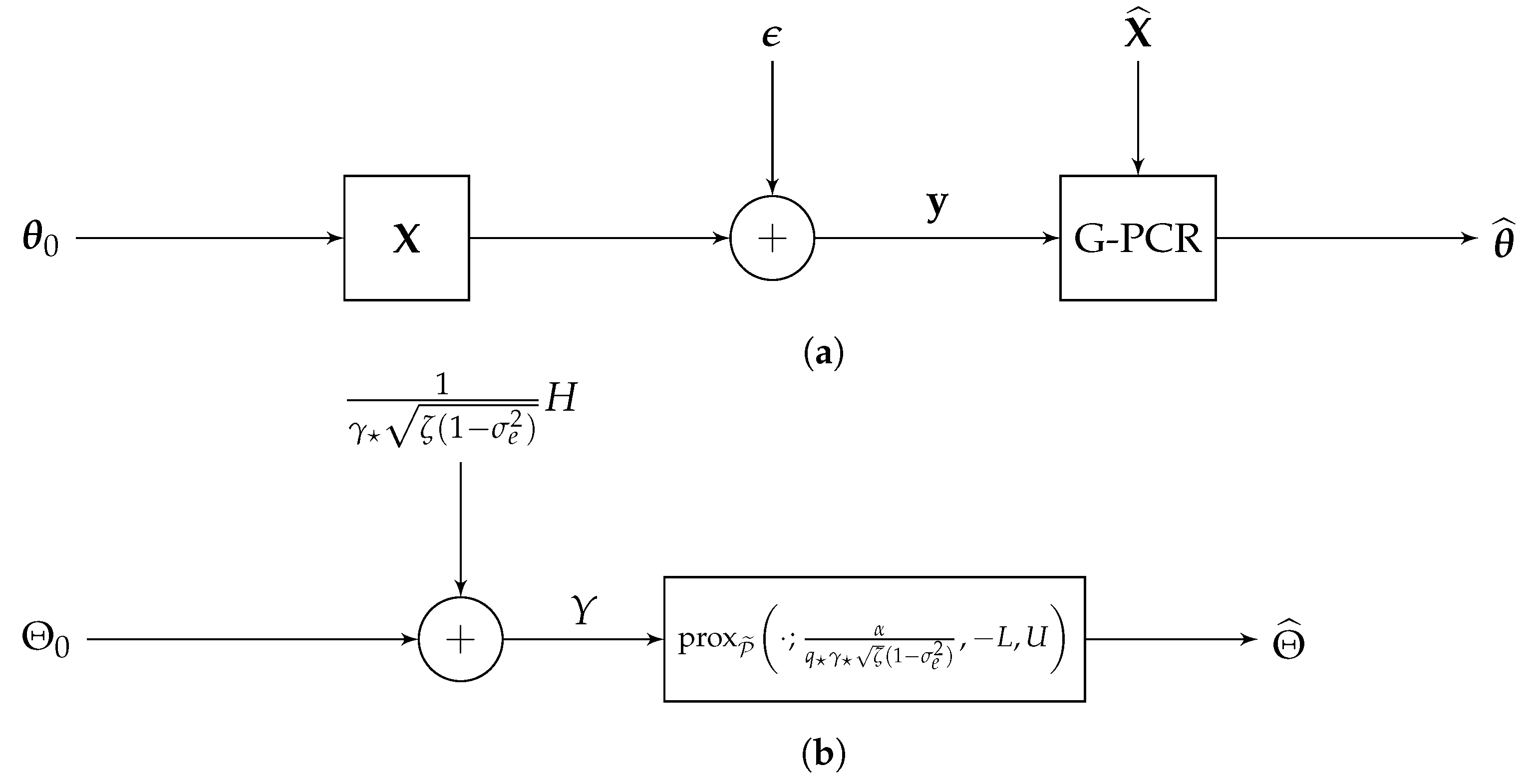
2. Problem Setup

2.1. Dataset Model

Consider the problem of estimating a scalar response $y_i$ from a set of n independent training data samples ${\left\{({\mathit{x}}_i,y_i)\right\}}_{i=1}^n$, where ${\mathit{x}}_i\in {\mathbb{R}}^p$ is the feature vector, following the linear model

$$\begin{array}{c}\hfill y_i={\mathit{\theta }}_0^{\top }{\mathit{x}}_i+{ϵ}_i,i\in \left[n\right],\end{array}$$

(7)

where ${\mathit{\theta }}_0\in {\mathbb{R}}^p$ is an unknown structured target vector, and ${\left\{{ϵ}_i\right\}}_{i=1}^n$ denotes the noise samples with zero mean and variance ${\sigma }_{ϵ}^2$. Furthermore, the feature vectors ${\mathit{x}}_i$ are assumed to independent and identically distributed (i.i.d.) random normal vectors with zero mean and covariance matrix $\frac{1}{p}{\mathbf{I}}_p$.

The model in (7) can be compactly written as

$$\mathbf{y}=\mathit{X}{\mathit{\theta }}_0+\mathit{ϵ},$$

where $\mathbf{y}={[y_1,y_2,\cdots ,y_n]}^{\top },\mathbf{X}={[{\mathit{x}}_1,{\mathit{x}}_2,\cdots ,{\mathit{x}}_n]}^{\top },$ and $\mathit{ϵ}={[{ϵ}_1,{ϵ}_2,\cdots ,{ϵ}_n]}^{\top }$.

2.2. Main Assumptions

Our study is based on the following set of assumptions:

• The unknown target vector ${\mathit{\theta }}_0$ is assumed to be a structured vector, with entries ${\mathrm{\Theta }}_0$ that are sampled i.i.d. from a probability distribution function $p_{\mathrm{\Theta }}$, which has zero mean, and variance $\mathbb{E}\left[{\mathrm{\Theta }}_0^2\right]={\sigma }_{\theta }^2$, where $0<{\sigma }_{\theta }^2<\infty$.
• The noise variance ${\sigma }_{ϵ}^2<\infty$ is a fixed positive constant.
• As discussed above, the data matrix $\mathbf{X}\in {\mathbb{R}}^{n\times p}$ is a Gaussian matrix with i.i.d. $\mathsf{N}(0,\frac{1}{p})$ elements. The choice of the $1/p$ as the variance level in X is commonly used in the literature; see [20,27]. This is done to ensure that ${\parallel \mathbf{X}\mathit{\theta }\parallel }_2^2/n$ and ${\parallel \mathit{\theta }\parallel }_2^2/p$ are of the same order.

Furthermore, in this work, we assume that the data matrix, X, is not perfectly known, and we only have an erroneous copy of it, $\widehat{\mathbf{X}}$, which is given as:

$$\widehat{\mathbf{X}}=\mathbf{X}+\mathbf{E},$$

(8)

where $\widehat{\mathbf{X}}$, and $\mathbf{E}\in {\mathbb{R}}^{n\times p}$ are independent matrices which have i.i.d. entries drawn from $\mathsf{N}(0,\frac{1-{\sigma }_e^2}{p})$, and $\mathsf{N}(0,\frac{{\sigma }_e^2}{p})$, respectively. (This uncertainty notion is widely encountered in practice. For example, it could be used to represent model mismatch, errors, and noises from the data collection process, noise in the sensors used to gather the measurements, etc.) Here, E represents the unknown error matrix, and ${\sigma }_e^2\in [0,1]$ is the variance of the error.

• n and p grow to infinity with $\frac{n}{p}⟶\zeta \in (0,\infty )$.

2.3. Generalized Penalized Constrained Regression (G-PCR)

In this paper, we refer to (5) as the standard G-PR, but we analyze a modified version that we call the Generalized Penalized Constrained Regression (G-PCR), which solves the following optimization instead:

$$\widehat{\mathit{\theta }}=arg\underset{\mathit{\theta }\in {\mathbb{V}}^p}{min}{\parallel \widehat{\mathbf{X}}\mathit{\theta }-\mathbf{y}\parallel }_2^2+\alpha \mathcal{P}\left(\mathit{\theta }\right),$$

(9)

where $\mathbb{V}=[-L,U],\mathrm{and}L,U\in {\mathbb{R}}_{+}\cup \left\{0\right\}.$

When compared to (6), the constraint $\mathbb{V}$ is used instead of $\mathbb{R}$, and $\widehat{\mathbf{X}}$ is used instead of X. This is due to the fact that X is not perfectly known and we only have its noisy estimate $\widehat{\mathbf{X}}$.

When we compare (9) to (6), we can see that there is only a slight difference between them, which is the constraint set $\mathbb{V}$ instead of $\mathbb{R}$. This small change assures significant performance improvements in the algorithm in many practical applications, such as image and signal processing [55], wireless communications [41,43,56], etc. These improvements are shown for several cases in Section 4 and Section 5.

3. Sharp Asymptotics

3.1. Measures of Performance

This paper considers the following measures used to assess the high-dimensional performance of the G-PCR.

• Prediction Risk: One of the most extensively used measures of performance is the prediction risk. For a given estimator $\widehat{\mathit{\theta }}$, the prediction risk is defined as

  $$\begin{array}{c}\hfill \mathsf{R}(\widehat{\mathit{\theta }},{\mathit{\theta }}_0):=\frac{1}{p}{\mathbb{E}}_{\mathit{x},y}\left[{\left|{\mathit{x}}^{\top }(\widehat{\mathit{\theta }}-{\mathit{\theta }}_0)\right|}^2\right]=\frac{1}{p}{\parallel \widehat{\mathit{\theta }}-{\mathit{\theta }}_0\parallel }_2^2,\end{array}$$

  (10)

  where x and y are new test points following the linear model in (7) but are independent of the training data.
• Similarity: Another metric that is used to quantify the degree of alignment between the target vector ${\mathit{\theta }}_0$ and its estimate $\widehat{\mathit{\theta }}$ is the (dis)similarity. It is a measure of orientation rather than magnitude. It is defined as

  $$\begin{array}{c}\hfill \varrho (\widehat{\mathit{\theta }},{\mathit{\theta }}_0):=\frac{{\widehat{\mathit{\theta }}}^{\top }{\mathit{\theta }}_0}{\parallel \widehat{\mathit{\theta }}{\parallel }_2\parallel {\mathit{\theta }}_0{\parallel }_2}\in [-1,1].\end{array}$$

  (11)

This similarity measure could also be thought of as the correlation between the estimated and true target vectors. Essentially, we desire estimates that maximize this similarity. Note that this metric is also known as the cosine similarity in machine learning literature, since $\varrho (\widehat{\mathit{\theta }},{\mathit{\theta }}_0)=cos(\angle (\widehat{\mathit{\theta }},{\mathit{\theta }}_0))$.

Note that these two measures are related as

$$\mathsf{R}(\widehat{\mathit{\theta }},{\mathit{\theta }}_0)=\frac{1}{p}\left[\parallel \widehat{\mathit{\theta }}{\parallel }_2^2+\parallel {\mathit{\theta }}_0{\parallel }_2^2-2\parallel \widehat{\mathit{\theta }}{\parallel }_2\parallel {\mathit{\theta }}_0{\parallel }_2\varrho (\widehat{\mathit{\theta }},{\mathit{\theta }}_0)\right].$$

3.2. High-Dimensional Performance Evaluation

In this subsection, we provide the main results of the paper, namely, the sharp analysis of the asymptotic performance of the G-PCR convex program. We start by analyzing the estimation performance via a general pseudo-Lipschitz function as in Theorem 1 below, which sharply characterizes the general asymptotic behavior of the error. Then, we use this theorem to compute particular performance measures such as the prediction risk, similarity, etc.

Theorem 1

(General Performance Metric). Consider the high-dimensional setup of Section 2.2, and let the assumptions therein hold. Moreover, let $\widehat{\mathit{\theta }}$ be a minimizer of the G-PCR program in (9) for a fixed $\alpha >0$. Let $\psi :\mathbb{R}\times \mathbb{R}\to \mathbb{R}$ be a pseudo-Lipschitz function. Then, in the limit of $p\to \infty$, it holds that

$$\begin{array}{c}\hfill \frac{1}{p}\sum _{j=1}^p\psi ({\widehat{\theta }}_j,{\theta }_{0,j})\stackrel{P}{⟶}\mathbb{E}\left[\psi \left({\mathrm{prox}}_{\tilde{\mathcal{P}}}\left({\mathrm{\Theta }}_0+\frac{H}{{\gamma }_{★}\sqrt{\zeta (1-{\sigma }_e^2)}};\frac{\alpha }{q_{★}{\gamma }_{★}\sqrt{\zeta }(1-{\sigma }_e^2)},-L,U\right),{\mathrm{\Theta }}_0\right)\right],\end{array}$$

(12)

where $(q_{★},{\gamma }_{★})$ is the unique optimal solution to the following objective,

$$\begin{array}{c}\hfill \begin{array}{cc}\underset{q\ge 0}{sup}\underset{\gamma >0}{inf}{\mathcal{O}}_{\tilde{\mathcal{P}}}(q,\gamma )\hfill & :=\frac{q\sqrt{\zeta }}{2\gamma }+\frac{q\gamma \sqrt{\zeta }}{2}\left({\sigma }_{ϵ}^2+{\sigma }_e^2{\sigma }_{\theta }^2\right)-\frac{q}{2\gamma \sqrt{\zeta }}-\frac{q^2}{4}\hfill \\ \hfill & +q\gamma \sqrt{\zeta }(1-{\sigma }_e^2)\mathbb{E}\left[{\mathsf{M}}_{\tilde{\mathcal{P}}}\left({\mathrm{\Theta }}_0+\frac{H}{\gamma \sqrt{\zeta (1-{\sigma }_e^2)}};\frac{\alpha }{q\gamma \sqrt{\zeta }(1-{\sigma }_e^2)},-L,U\right)\right],\hfill \end{array}\end{array}$$

(13)

and the expectation is taken with respect to independent random variables ${\mathrm{\Theta }}_0\sim p_{\mathrm{\Theta }}$ and $H\sim \mathsf{N}(0,1)$.

Proof. 

The proof is given in Appendix A. □

Remark 1

(Choice of $\psi (·,·)$). The performance metric in Theorem 1 is computed in terms of evaluation of a pseudo-Lipschitz function, $\psi (·,·)$. As an example, $\psi (a,b)={(a-b)}^2$ can be used to compute the prediction risk, or $\psi (a,b)=|a-b|$ can be used to evaluate the mean absolute error (MAE). We will appeal to this theorem later with various choices of $\psi (·,·)$ to evaluate different performance measures on $\widehat{\mathit{\theta }}$.

Remark 2

(Optimal Solutions). Note that $q_{★}$ and ${\gamma }_{★}$ can be calculated by any search technique such as the golden-section search method and the ternary search [57].

Remark 3

(Decoupling Property). Theorem 1 shows that

$$\begin{array}{c}\hfill \frac{1}{p}\sum _{j=1}^p\psi ({\widehat{\theta }}_j,{\theta }_{0,j})\stackrel{P}{⟶}\mathbb{E}\left[\psi (\widehat{\mathrm{\Theta }},{\mathrm{\Theta }}_0)\right],\end{array}$$

(14)

where

$$\begin{array}{c}\hfill \widehat{\mathrm{\Theta }}:={\mathrm{prox}}_{\tilde{\mathcal{P}}}\left(\underset{:=Y}{\underbrace{{\mathrm{\Theta }}_0+\frac{H}{{\gamma }_{★}\sqrt{\zeta (1-{\sigma }_e^2)}}}};\frac{\alpha }{q_{★}{\gamma }_{★}\sqrt{\zeta }(1-{\sigma }_e^2)},-L,U\right).\end{array}$$

(15)

This provides some insights for the structured signal recovery with the G-PCR optimization. From (14), it can be seen that the random variable $\widehat{\mathrm{\Theta }}$ shares the same statistical properties as the estimate $\widehat{\mathit{\theta }}$ [46]. Thus, Equation (15) can be considered as a decoupled scalar version of the original system as depicted in Figure 1. Particularly, in the original system (Figure 1a), the true target vector ${\mathit{\theta }}_0$ is first mixed by the design matrix X, and then the additive white Gaussian noise (AWGN) vector ϵ is added to form the measurement vector y. On the other hand, in the decoupled system (Figure 1b), the unknown variable ${\mathrm{\Theta }}_0$ is only mixed by the Gaussian vector $\frac{1}{{\gamma }_{★}\sqrt{\zeta (1-{\sigma }_e^2)}}H$, where $Y:={\mathrm{\Theta }}_0+\frac{1}{{\gamma }_{★}\sqrt{\zeta (1-{\sigma }_e^2)}}H$. Furthermore, letting $B:=\frac{1}{q_{★}{\gamma }_{★}\sqrt{\zeta }(1-{\sigma }_e^2)}$, it can be observed that the generalized proximal operator solution

$$\widehat{\mathrm{\Theta }}={\mathrm{prox}}_{\tilde{\mathcal{P}}}\left(Y;\alpha B,-L,U\right)=\underset{-L\le \theta \le U}{\arg \min }\frac{1}{2}{(Y-\theta )}^2+\alpha B\tilde{\mathcal{P}}\left(\theta \right)$$

has a decoupled scalar form of the original G-PCR in (9), which can be expressed as

$$\widehat{\mathit{\theta }}=\underset{-L\le {\theta }_j\le U}{\arg \min }\frac{1}{2}\parallel \mathbf{y}-\widehat{\mathbf{X}}\mathit{\theta }{\parallel }_2^2+\alpha B\mathcal{P}\left(\mathit{\theta }\right),j\in \left[p\right]$$

up to a scaling of B. This suggests that, in the high-dimensional asymptotic setting, one can use the decoupled scalar system to characterize the probabilistic properties of the G-PCR recovery problem.

This decoupling property was also shown for similar problems, such as box-constrained sum of absolute values (Box-SOAV) optimization for sparse recovery [46], sparse logistic regression [58], and the approximate message passing (AMP) algorithm [59].

As a first application of Theorem 1, we provide a sharp high-dimensional performance evaluation of the prediction risk as given in the following corollary.

Corollary 1

(Prediction Risk). Under the same assumptions of Theorem 1, and for ${\mathrm{\Theta }}_0\sim p_{\mathrm{\Theta }}$ that is independent of $H\sim \mathsf{N}(0,1)$, it holds that

$$\begin{array}{c}\hfill \begin{array}{cc}\mathsf{R}(\widehat{\mathit{\theta }},{\mathit{\theta }}_0)\stackrel{P}{⟶}\hfill & {\mathbb{E}}_{{\mathrm{\Theta }}_0,H}\left[{\left({\mathrm{prox}}_{\tilde{\mathcal{P}}}\left({\mathrm{\Theta }}_0+\frac{H}{{\gamma }_{★}\sqrt{\zeta (1-{\sigma }_e^2)}};\frac{\alpha }{q_{★}{\gamma }_{★}\sqrt{\zeta }(1-{\sigma }_e^2)},-L,U\right)-{\mathrm{\Theta }}_0\right)}^2\right]\hfill \\ \hfill & =\frac{1}{1-{\sigma }_e^2}\left(\frac{1}{{\gamma }_{★}^2}-{\sigma }_{\theta }^2{\sigma }_e^2-{\sigma }_{ϵ}^2\right),\hfill \end{array}\end{array}$$

(16)

where $q_{★}$ and ${\gamma }_{★}$ are the unique optimal solutions to the objective function in (13).

Proof. 

Using Theorem 1 with $\psi (a,b)={(a-b)}^2$, we can obtain the above expression of the prediction risk. Details are deferred to Appendix A.2.4. □

Remark 4

(Optimal Hyper-parameters). Corollary 1 allows us to determine the optimal hyper-parameters, such as $\alpha ,L$, and U, that minimize the prediction risk. To do so, it is first required to estimate some variances, such as ${\sigma }_{\theta }^2,{\sigma }_{ϵ}^2$ and ${\sigma }_e^2$, from the available data. Those can be easily estimated by using existing algorithms such as [60,61].

It should be noted that this theoretical hyper-parameter optimal tuning as discussed above avoids the traditional time/data-consuming practice of cross-validation used to tune the hyper parameters.

The following corollary sharply characterizes the similarity measure defined earlier in (11).

Corollary 2

(Similarity). Under the same assumptions and settings of Theorem 1, and in the limit of $p\to \infty$, it holds that

$$\varrho (\widehat{\mathit{\theta }},{\mathit{\theta }}_0)\stackrel{P}{⟶}\frac{{\mathbb{E}}_{{\mathrm{\Theta }}_0,H}\left[{\mathrm{prox}}_{\tilde{\mathcal{P}}}\left({\mathrm{\Theta }}_0+\frac{H}{{\gamma }_{★}\sqrt{\zeta (1-{\sigma }_e^2)}};\frac{\alpha }{q_{★}{\gamma }_{★}\sqrt{\zeta }(1-{\sigma }_e^2)},-L,U\right){\mathrm{\Theta }}_0\right]}{\sqrt{{\sigma }_{\theta }^2·{\mathbb{E}}_{{\mathrm{\Theta }}_0,H}\left[{\mathrm{prox}}_{\tilde{\mathcal{P}}}^2\left({\mathrm{\Theta }}_0+\frac{H}{{\gamma }_{★}\sqrt{\zeta (1-{\sigma }_e^2)}};\frac{\alpha }{q_{★}{\gamma }_{★}\sqrt{\zeta }(1-{\sigma }_e^2)},-L,U\right)\right]}},$$

(17)

where $q_{★}$ and ${\gamma }_{★}$ are the unique optimal solutions to (13).

Proof. 

The proof follows from Theorem 1 and from the continuous mapping Theorem [62]. Details are given in Appendix A.2.5. □

In the subsequent sections, we consider various instants of (9), such as ${\mathcal{l}}_1$-norm and ${\mathcal{l}}_2$-norm penalization, to illustrate the application of the theoretical asymptotic expressions derived in this section.

4. Sparse Linear Regression

In this section, we study the performance of the G-PCR with an ${\mathcal{l}}_1$-norm penalization. As indicated in the introduction, this penalty function is used to promote sparse solutions. In contemporary machine learning applications, it is common to encounter a significantly large number of features, p. To prevent the problem of over-fitting, it becomes crucial to engage in feature selection, which involves eliminating irrelevant variables from the regression model [18]. A popular technique for accomplishing this is by introducing an ${\mathcal{l}}_1$-norm penalty to the loss function. This approach is widely adopted and used for feature selection tasks.

Therefore, we specialize Theorem 1 to analyze the asymptotic performance of the G-PCR with an ${\mathcal{l}}_1$-norm penalization. Particularly, for an s-sparse vector, we study the performance of the following optimization problem:

$$\widehat{\mathit{\theta }}=\arg \underset{-L\le {\theta }_j\le U}{min}\parallel {\widehat{\mathbf{X}}\mathit{\theta }-\mathbf{y}\parallel }_2^2+\alpha {\parallel \mathit{\theta }\parallel }_1,j\in \left[p\right].$$

(18)

(We say that a vector v $\in {\mathbb{R}}^p$ is an s-sparse vector if only s of its p elements are non-zero (on average), and most of its elements are zeros, where $s\ll p$.)

4.1. Asymptotic Behavior of Sparse G-PCR

To analyze (18), we specialize Theorem 1 with $\tilde{\mathcal{P}}(·)=| · |$. Then, the generalized proximal operator and Moreau envelope functions can be expressed, respectively, in the following closed forms:

$${\mathrm{prox}}_{|·|}(x;b,c,d):={\eta }_1(x;b,c,d)=\left\{\begin{array}{cc}d\hfill & ,\mathrm{if}x\ge d+b\hfill \\ x-b\hfill & ,\mathrm{if}b<x<d+b\hfill \\ 0\hfill & ,\mathrm{if}\left|x\right|\le b\hfill \\ x+b\hfill & ,\mathrm{if}c-b<x<-b\hfill \\ c\hfill & ,\mathrm{if}x\le c-b,\hfill \end{array}\right.$$

(19)

and

$${\mathsf{M}}_{|·|}(x;b,c,d)=\left\{\begin{array}{cc}\frac{1}{2}{(d-x)}^2+bd\hfill & ,\mathrm{if}x\ge d+b\hfill \\ bx-\frac{1}{2}{b}^2\hfill & ,\mathrm{if}b<x<d+b\hfill \\ \frac{1}{2}{x}^2\hfill & ,\mathrm{if}\left|x\right|\le b\hfill \\ -bx-\frac{1}{2}{b}^2\hfill & ,\mathrm{if}c-b<x<-b\hfill \\ \frac{1}{2}{(c-x)}^2-bc\hfill & ,\mathrm{if}x\le c-b.\hfill \end{array}\right.$$

(20)

Note that this proximal operator is a generalization of the well-known soft-thresholding operator, i.e., $\eta (x;b)=\mathrm{sign}\left(x\right)\mathrm{ReLU}\left(\right|x|-b)$, where the Rectified Linear Unit ($\mathrm{ReLU}$) is defined as $\mathrm{ReLU}\left(t\right)=max(0,t)$.

These expressions can be used to solve the scalar optimization in (13) of Theorem 1 and to simplify the similarity expression in (17). Specifically, (13) becomes

$$\begin{array}{c}\hfill \begin{array}{cc}\underset{q\ge 0}{sup}\underset{\gamma >0}{inf}{\mathcal{O}}_{|·|}(q,\gamma )\hfill & =\frac{q\sqrt{\zeta }}{2\gamma }+\frac{q\gamma \sqrt{\zeta }}{2}\left({\sigma }_{ϵ}^2+{\sigma }_e^2{\sigma }_{\theta }^2\right)-\frac{q}{2\gamma \sqrt{\zeta }}-\frac{q^2}{4}\hfill \\ \hfill & +q\gamma \sqrt{\zeta }(1-{\sigma }_e^2)\mathbb{E}\left[{\mathsf{M}}_{|·|}\left({\mathrm{\Theta }}_0+\frac{H}{\gamma \sqrt{\zeta (1-{\sigma }_e^2)}};\frac{\alpha }{q\gamma \sqrt{\zeta }(1-{\sigma }_e^2)},-L,U\right)\right].\hfill \end{array}\end{array}$$

(21)

Figure 2 illustrates the performance of the ${\mathcal{l}}_1$-penalized G-PCR as a function of $\alpha$ for different levels of error variance ${\sigma }_e^2$. We generated the target vector ${\mathit{\theta }}_0$ randomly with elements in $\{-1,0,+1\}$ and $\mathbb{P}({\theta }_{0,j}=-1)=\mathbb{P}({\theta }_{0,j}=+1)=0.2$. This means that the sparsity factor $\rho :=\frac{s}{p}$ is $0.2$ in these simulations. From these figures, we can also see that the theoretical expressions of the prediction risk and the similarity match the empirical simulations very well. Furthermore, it can be noted in Figure 2a that, for different values of ${\sigma }_e^2$, there exists an optimal value ${\alpha }_{★}$ that achieves the minimum possible prediction risk. Similarly, notice in Figure 2b the optimal ${\alpha }_{★}$ that maximizes the similarity metric. It can also be observed that increasing $\alpha$ beyond ${\alpha }_{★}$ reduces the similarity $\varrho$ between $\widehat{\mathit{\theta }}$ and ${\mathit{\theta }}_0$. In these simulations, we set $-L=min\left({\mathit{\theta }}_0\right)=-1$ and $U=max\left({\mathit{\theta }}_0\right)=+1$.

In Figure 3, we compare the unconstrained G-PR in (6) (which is equivalent to a standard LASSO formulation in this case) to the proposed G-PCR for an over-parameterized setting with $\zeta =0.85$. As we can see from this figure, the G-PCR clearly outperforms the unconstrained one in both metrics. Moreover, despite the fact that our theoretical results are assumed to be asymptotic in the problem dimensions (i.e., $n\to \infty$ and $p\to \infty$), we can see from all of the above figures that our rigorous results are accurate even for problems with a few hundred variables, e.g., $p=300$.

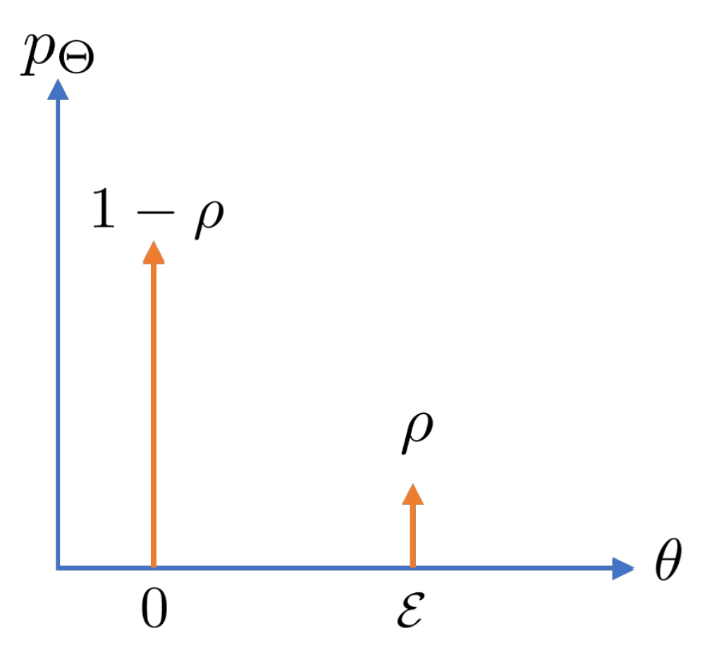
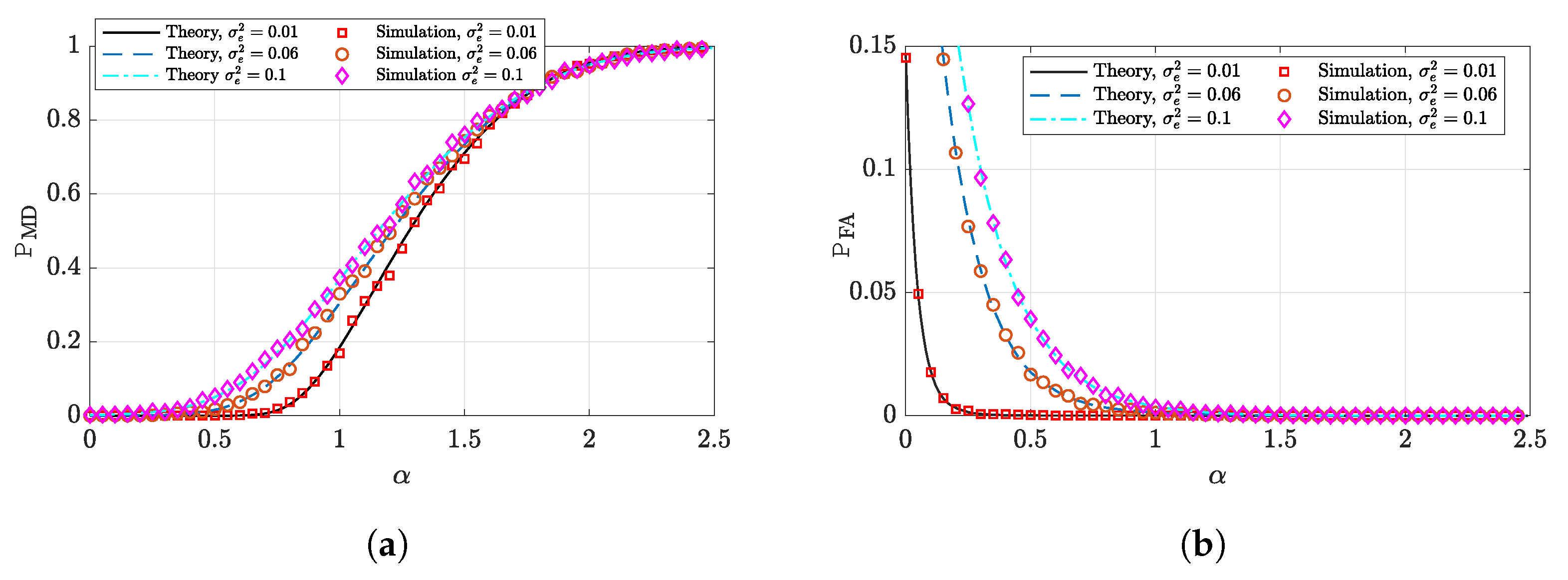
4.2. Support Recovery

In this section, we analyze the so-called support recovery of the sparse G-PCR. As discussed earlier, a sparse vector means that it has few non-zero elements. We define the support of ${\mathit{\theta }}_0$ as follows:

$$\mathrm{\Omega }:=\{j\in \left[p\right]|{\theta }_{0,j}\ne 0\}\subseteq \left[p\right].$$

Here, we are interested in computing the probability that an element on the support of ${\mathit{\theta }}_0$ has been recovered correctly. Let $\widehat{\mathit{\theta }}$ be a solution to the optimization problem in (18). Let us fix $\xi >0$ as a user-predefined hard threshold based on whether an entry of $\widehat{\mathit{\theta }}$ is decided to be on the support or not. Formally, we construct the following set as the estimate of the support given $\widehat{\mathit{\theta }}$:

$${\widehat{\mathrm{\Omega }}}_{\xi }:=\{j\in \left[p\right]||{\widehat{\theta }}_j|>\xi \}.$$

In order to analyze the support recovery correctness, we consider the following error metrics, which are known as the probability of misdetection (MD) and the probability of false alarm (FA), respectively.

$${\mathsf{P}}_{\mathrm{MD}}\left(\xi \right)=\mathbb{P}(j\notin {\widehat{\mathrm{\Omega }}}_{\xi }|j\in \mathrm{\Omega }),\mathrm{and}{\mathsf{P}}_{\mathrm{FA}}\left(\xi \right)=\mathbb{P}(j\in {\widehat{\mathrm{\Omega }}}_{\xi }|j\notin \mathrm{\Omega }).$$

In the following lemma, we study the asymptotic performance of both of these measures.

Lemma 1.

Let $\widehat{\mathit{\theta }}$ be a solution to (18), and assume that ${\mathit{\theta }}_0$ is a sparse signal. Fix $\alpha >0$ and $\xi >0$. Then, in the limit of $p\to \infty$, it holds that

$$\begin{array}{cc}\hfill {\mathsf{P}}_{\mathrm{MD}}\left(\xi \right)\stackrel{P}{⟶}& \mathbb{P}\left(\left|{\eta }_1\left({\mathrm{\Theta }}_0+\frac{H}{{\gamma }_{★}\sqrt{\zeta (1-{\sigma }_e^2)}};\frac{\alpha }{q_{★}{\gamma }_{★}\sqrt{\zeta }(1-{\sigma }_e^2)},-L,U\right)\right|\le \xi \right),\hfill \end{array}$$

(22)

and

$$\begin{array}{cc}\hfill {\mathsf{P}}_{\mathrm{FA}}\left(\xi \right)\stackrel{P}{⟶}& \mathbb{P}\left(\left|{\eta }_1\left(\frac{H}{{\gamma }_{★}\sqrt{\zeta (1-{\sigma }_e^2)}};\frac{\alpha }{q_{★}{\gamma }_{★}\sqrt{\zeta }(1-{\sigma }_e^2)},-L,U\right)\right|\ge \xi \right),\hfill \end{array}$$

(23)

where ${\eta }_1(·;·,·,·)$ is as defined in (19), $(q_{★},{\gamma }_{★})$ is the unique optimal solution to (21), and the probabilities are taken with respect to the randomness of ${\mathrm{\Theta }}_0$ and $H\sim \mathsf{N}(0,1)$.

Proof. 

The proof can be obtained from Theorem 1 with some approximations of these metrics to Lipschitz functions. Details are omitted for briefness. See [39] for a similar proof. □

Next, we give an example to illustrate this lemma.

Example: Sparse-Binary Target Vectors

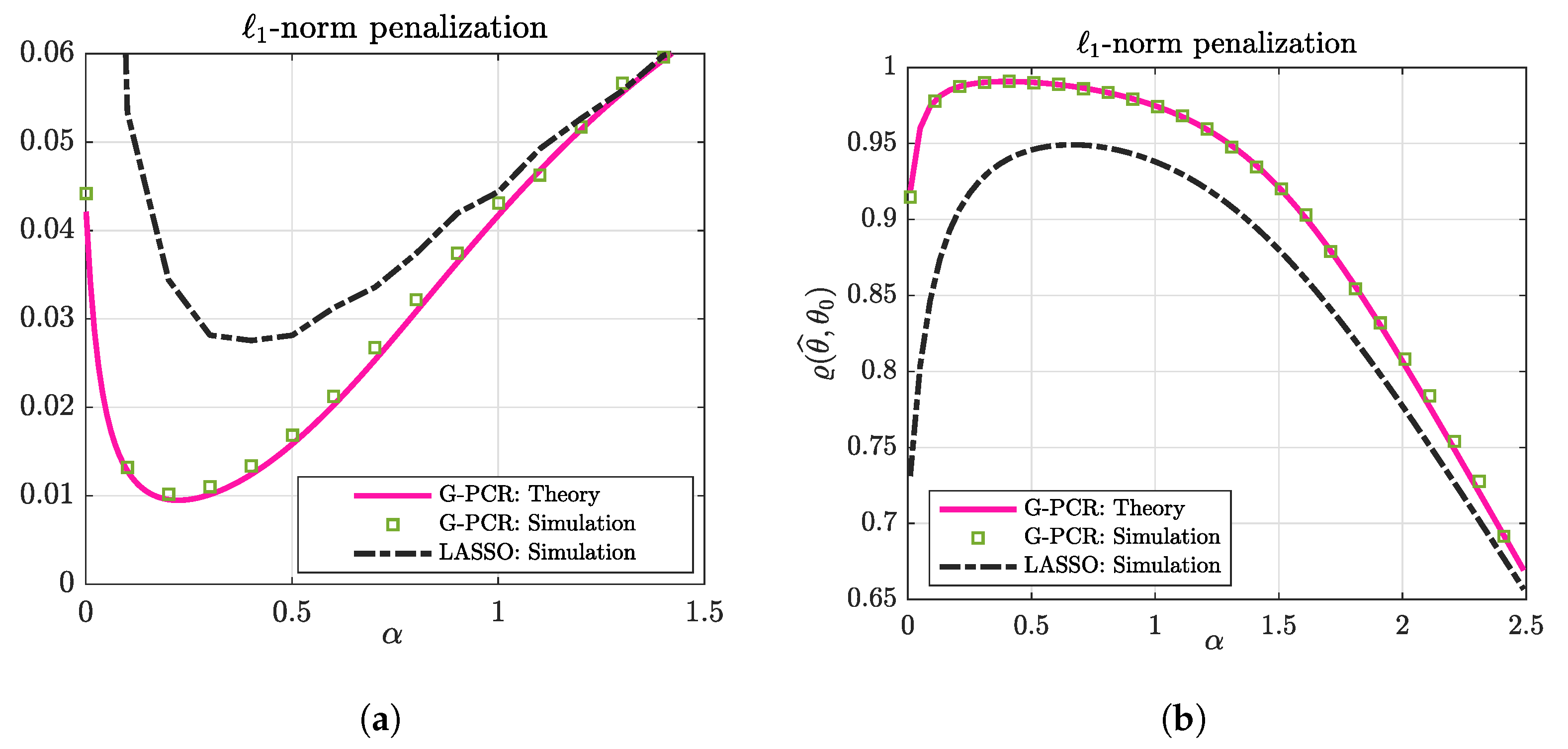
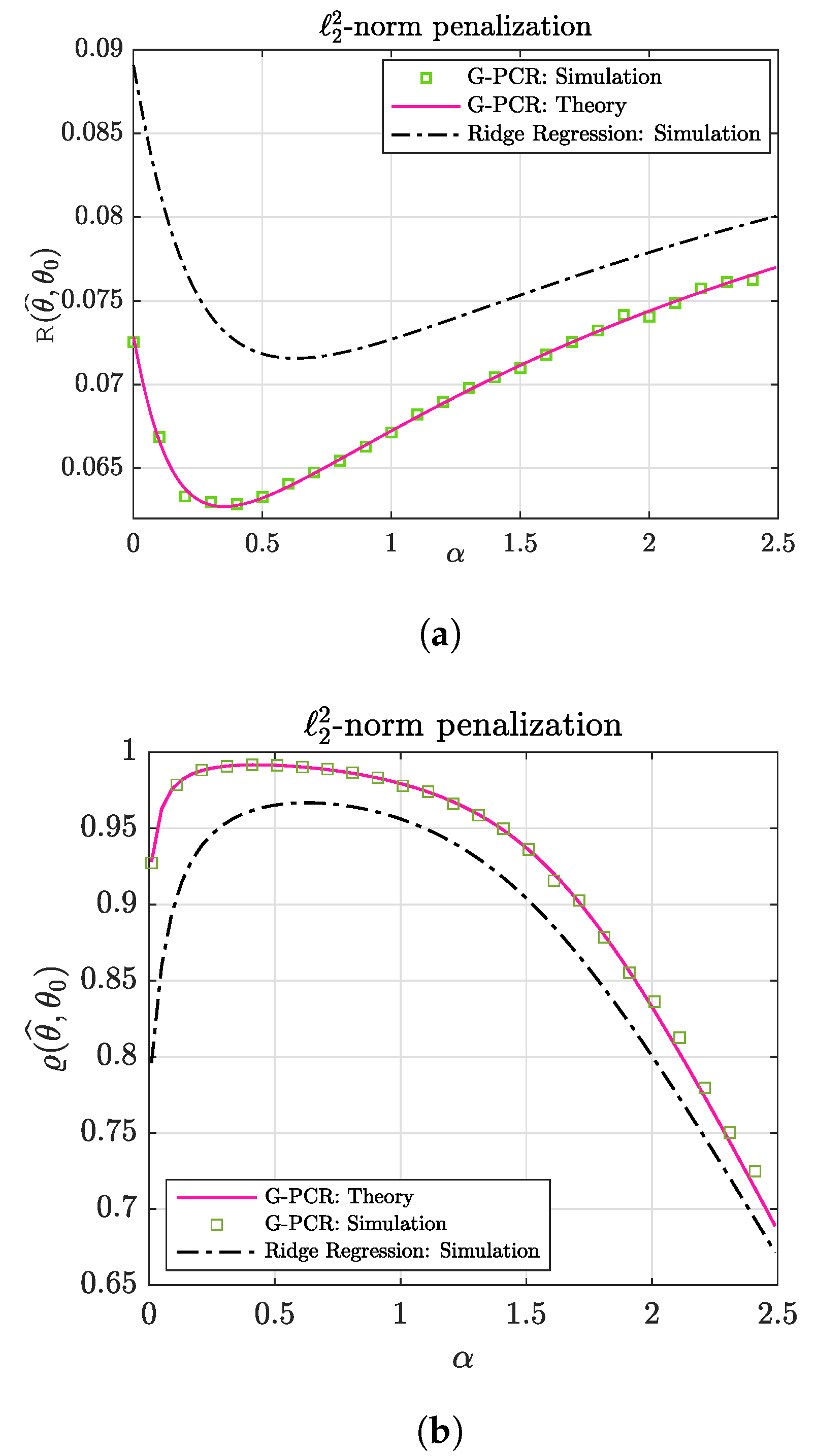
For an s-sparse target vector, define $\rho :=\frac{s}{p}\in (0,1]$ as the sparsity factor. Then, as an example, let us assume that each element ${\theta }_{0,j}$, for $j\in \left[p\right]$, is i.i.d. drawn from the following distribution (this model has been widely adopted in the relevant literature; see, for example, [59,63,64]):

$$\begin{array}{c}\hfill p_{\mathrm{\Theta }}\left(\theta \right)=(1-\rho ){\delta }_0\left(\theta \right)+\rho {\delta }_0(\theta -\mathcal{E}),\end{array}$$

(24)

for some $\mathcal{E}>0$, and ${\delta }_0(·)$ indicates a Dirac delta function (i.e., a point-mass distribution). In other words, the elements of ${\mathit{\theta }}_0$ are zero with probability $1-\rho$, and the non-zero elements all have the value $\mathcal{E}$. Figure 4 illustrates this distribution.

For a ${\mathrm{\Theta }}_0$ that follows the distribution in (24), and for $\xi \in (0,\mathcal{E})$, with $L=0$ and $U=\mathcal{E}$, the error measures in Lemma 1 simplify to the following:

$$\begin{array}{c}\hfill {\mathsf{P}}_{\mathrm{MD}}\stackrel{P}{⟶}\mathrm{\Phi }\left((\xi -\mathcal{E}){\gamma }_{★}\sqrt{\zeta (1-{\sigma }_e^2)}+\frac{\alpha }{q_{★}\sqrt{1-{\sigma }_e^2}}\right),\end{array}$$

(25)

and

$$\begin{array}{c}\hfill {\mathsf{P}}_{\mathrm{FA}}\stackrel{P}{⟶}1-\mathrm{\Phi }\left(\xi {\gamma }_{★}\sqrt{\zeta (1-{\sigma }_e^2)}+\frac{\alpha }{q_{★}\sqrt{1-{\sigma }_e^2}}\right),\end{array}$$

(26)

where $\mathrm{\Phi }\left(t\right)=\frac{1}{\sqrt{2\pi }}{\int }_{-\infty }^t{e}^{-u^2}\mathrm{d}u$ is the cumulative distribution function (CDF) of the standard normal distribution.

Figure 5 shows the accuracy of the above-derived theoretical expressions as compared to empirical simulations for the considered sparse-binary vector example.

5. G-PCR with ${\ell }_{\mathbf{2}}^{\mathbf{2}}$-Norm Penalization

Even though it does not promote a particular structure, ${\mathcal{l}}_2$-norm penalization is used in many signal processing, statistics, and machine learning applications to stabilize the model when we have ill-conditioned or under-determined systems [17]. Adding this penalization will shrink all the coefficients toward zero and hence decrease the variance of the resultant model; therefore, it can be used to avoid over-fitting. Within the Bayesian framework, the incorporation of this penalization implies that the regression coefficients are assumed to follow a Gaussian distribution. This assumption is often justifiable in numerous applications, in which the regression coefficients are typically taken from a random process. In this section, we provide high-dimensional asymptotic performance analysis of the G-PCR with ${\mathcal{l}}_2^2$-norm penalization; that is:

$$\widehat{\mathit{\theta }}=\arg \underset{-L\le {\theta }_j\le U}{min}\parallel \widehat{\mathbf{X}}\mathit{\theta }{-\mathbf{y}\parallel }_2^2+\alpha {\parallel \mathit{\theta }\parallel }_2^2,j\in \left[p\right].$$

(27)

To analyze (27), we use Theorem 1. However, here the generalized proximal operator and Moreau envelope functions of $\tilde{\mathcal{P}}(·)={(·)}^2$ can be expressed, respectively, in the following closed-forms:

$${\mathrm{prox}}_{{(·)}^2}(x;b,c,d)=\left\{\begin{array}{cc}\frac{x}{1+2b},\hfill & \mathrm{if}c\le x\le d\hfill \\ c,\hfill & \mathrm{if}x<c\hfill \\ d,\hfill & \mathrm{if}x>d,\hfill \end{array}\right.$$

(28)

and

$${\mathsf{M}}_{{(·)}^2}(x;b,c,d)=\left\{\begin{array}{cc}\frac{b{x}^2}{1+2b},\hfill & \mathrm{if}c\le x\le d\hfill \\ \frac{1}{2}{(x-c)}^2+b{c}^2,\hfill & \mathrm{if}x<c\hfill \\ \frac{1}{2}{(x-d)}^2+b{d}^2,\hfill & \mathrm{if}x>d.\hfill \end{array}\right.$$

(29)

Letting $b=\frac{\alpha }{q\gamma \sqrt{\zeta }(1-{\sigma }_e^2)}$ and $\lambda =\gamma \sqrt{\zeta (1-{\sigma }_e^2)}$, the scalar optimization in (13) of Theorem 1 reduces to:

$$\begin{array}{c}\hfill \begin{array}{cc}\underset{q\ge 0}{sup}\underset{\gamma >0}{inf}{\mathcal{O}}_{{(·)}^2}(q,\gamma )\hfill & =\frac{q\sqrt{\zeta }}{2\gamma }+\frac{q\gamma \sqrt{\zeta }}{2}\left({\sigma }_{ϵ}^2+{\sigma }_e^2{\sigma }_{\theta }^2\right)-\frac{q}{2\gamma \sqrt{\zeta }}-\frac{q^2}{4}\hfill \\ \hfill & +q\gamma \sqrt{\zeta }(1-{\sigma }_e^2)\left\{\mathbb{E}\right[\frac{b}{1+2b}{\left({\mathrm{\Theta }}_0+\frac{H}{\lambda }\right)}^2{\mathbf{1}}_{\{-L\le {\mathrm{\Theta }}_0+\frac{H}{\lambda }\le U\}}\hfill \\ \hfill & +\left[\frac{1}{2}{\left({\mathrm{\Theta }}_0+\frac{H}{\lambda }+L\right)}^2+b{L}^2\right]{\mathbf{1}}_{\{{\mathrm{\Theta }}_0+\frac{H}{\lambda }\le -L\}}\hfill \\ \hfill & +\left[\frac{1}{2}{\left({\mathrm{\Theta }}_0+\frac{H}{\lambda }-U\right)}^2+b{U}^2\right]{\mathbf{1}}_{\{{\mathrm{\Theta }}_0+\frac{H}{\lambda }\ge U\}}\left]\right\},\hfill \end{array}\end{array}$$

(30)

where ${\mathbf{1}}_{\{·\}}$ is the indicator function.

In the same manner, we can simplify the similarity expression in (17) using the closed-form expression of the generalized proximal operator of the ${\mathcal{l}}_2^2$-norm in (28). The prediction risk and the similarity metric are given by (16) and (17), respectively. However, now $(q_{★},{\gamma }_{★})$ is the unique solution to (30). To illustrate the ideal let us consider the next examples.

5.1. Numerical Illustration

As stated at the beginning of this section, ${\mathcal{l}}_2$-norm penalization can be used for Gaussian distributed target vectors. Therefore, as a first illustration, let us assume that ${\theta }_{0,j}$$\sim \mathsf{N}(0,1)\forall j\in \left[p\right]$. Figure 6 depicts the risk/similarity performance of the G-PCR with an ${\mathcal{l}}_2$-norm penalization for several levels of the penalization factor $\alpha$. It also shows that the G-PCR outperforms the unconstrained G-PR, which is equivalent to a ridge regression formulation here. Again, Figure 6a illustrates that there exists an optimal value ${\alpha }_{★}$ that minimizes prediction risk, while Figure 6b shows that there is an optimal value of the penalization factor ${\alpha }_{★}$ that gives the maximum similarity. Both figures show the high accuracy of the derived asymptotic expressions as compared to Monte Carlo simulations.

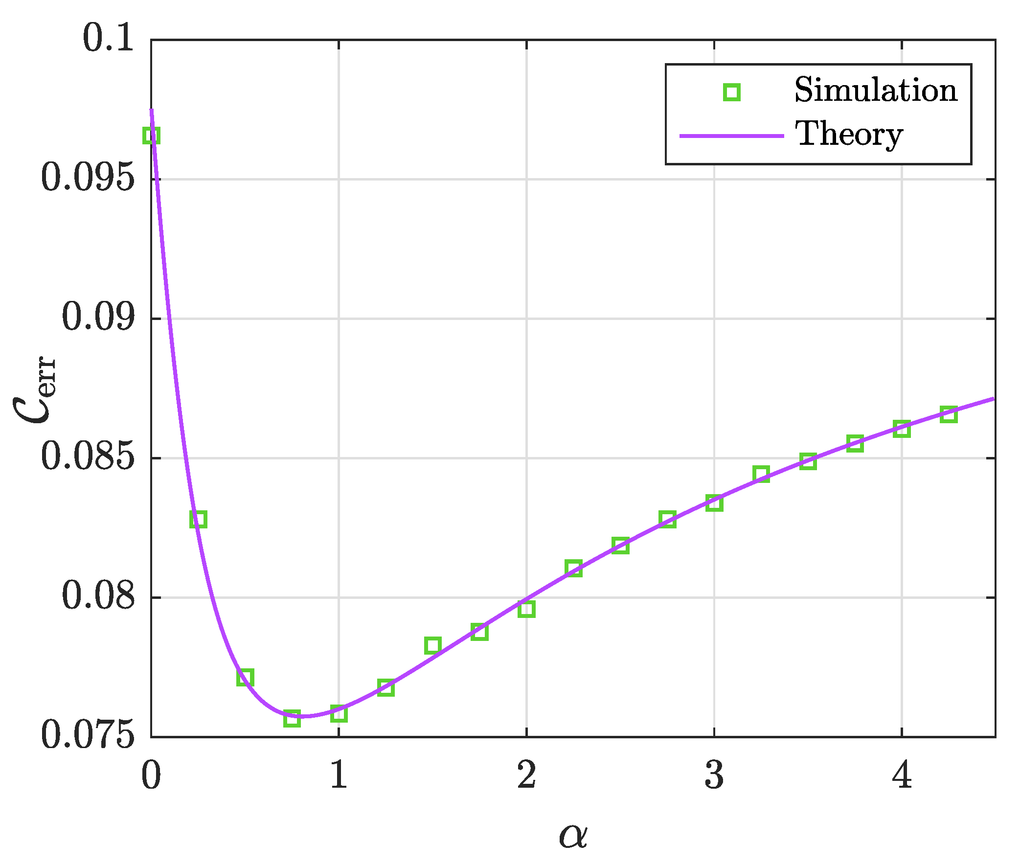
5.2. Binary Target Vector Estimation

Let us assume that ${\mathit{\theta }}_0={\{\pm 1\}}^p$, i.e., it takes only one of two possible values, $+1$ or $-1$, with equal probability, i.e.,

$$\begin{array}{c}\hfill p_{\mathrm{\Theta }}\left(\theta \right)=\frac{1}{2}\left[{\delta }_0(\theta -1)+{\delta }_0(\theta +1)\right].\end{array}$$

(31)

Such vectors are widely encountered in many practical applications, such as the detection of wireless communication signals [12,41]. We use (27) as our estimation method, with $L=U=1$. For this vector, ${\sigma }_{\theta }^2=1$; i.e., the covariance matrix of ${\mathit{\theta }}_0$ is ${\mathbf{C}}_{\theta }={\mathbf{I}}_p$.

The task of estimating ${\mathit{\theta }}_0$ here is equivalent to a binary classification task, with the two classes being $+1$ and $-1$. After obtaining the estimates using (27), we can map (decode) them to the relative class using the following link function:

$$\overline{\mathit{\theta }}=\mathrm{sign}\left(\widehat{\mathit{\theta }}\right).$$

We can use the prediction risk and similarity to measure the performance. However, a more suitable performance measure for this kind of target vector is the so-called “classification error rate”, which is defined as:

$$\begin{array}{c}\hfill {\mathcal{C}}_{\mathrm{err}}:=\frac{1}{p}\sum _{j=1}^p{\mathbf{1}}_{\{{\overline{\theta }}_j\ne {\theta }_{0,j}\}}.\end{array}$$

(32)

The next lemma derives an asymptotic expression for this metric.

Lemma 2.

Let $\widehat{\mathit{\theta }}$ be a solution to (27), and assume that ${\mathit{\theta }}_0={\{\pm 1\}}^p$, with a PMF $p_{\mathrm{\Theta }}$ that follows (31). Fix $\zeta >0$. Then, in the limit of $p\to \infty$, it holds that

$$\begin{array}{c}\hfill {\mathcal{C}}_{\mathrm{err}}\stackrel{P}{⟶}1-\mathrm{\Phi }\left({\gamma }_{★}\sqrt{\zeta (1-{\sigma }_e^2)}\right),\end{array}$$

(33)

where ${\gamma }_{★}$ is the optimal solution of (30) in γ.

Proof. 

The proof is similar to that of Lemma 1. Please refer to [39,47]. Details are skipped for brevity. □

Figure 7 illustrates the sharpness of Lemma 2 as compared to empirical simulations. Similar to previous figures, this figure demonstrates the perfect match between numerical simulations and theory.

5.3. Unpenalized Regression

When $\alpha =0$ in (9), we have an optimization problem with no penalization. The resulting algorithm is known as the box relaxation optimization (BRO) [39], which has been extensively studied in the literature. It is used to promote boundedness structure. In fact, when $L=U$, the BRO is equivalent to an ${\mathcal{l}}_{\infty }$-norm penalization. Setting $\alpha =0$ in (30), and after some mapping of the involved variables, we can obtain the same results as in [39] for binary vectors.

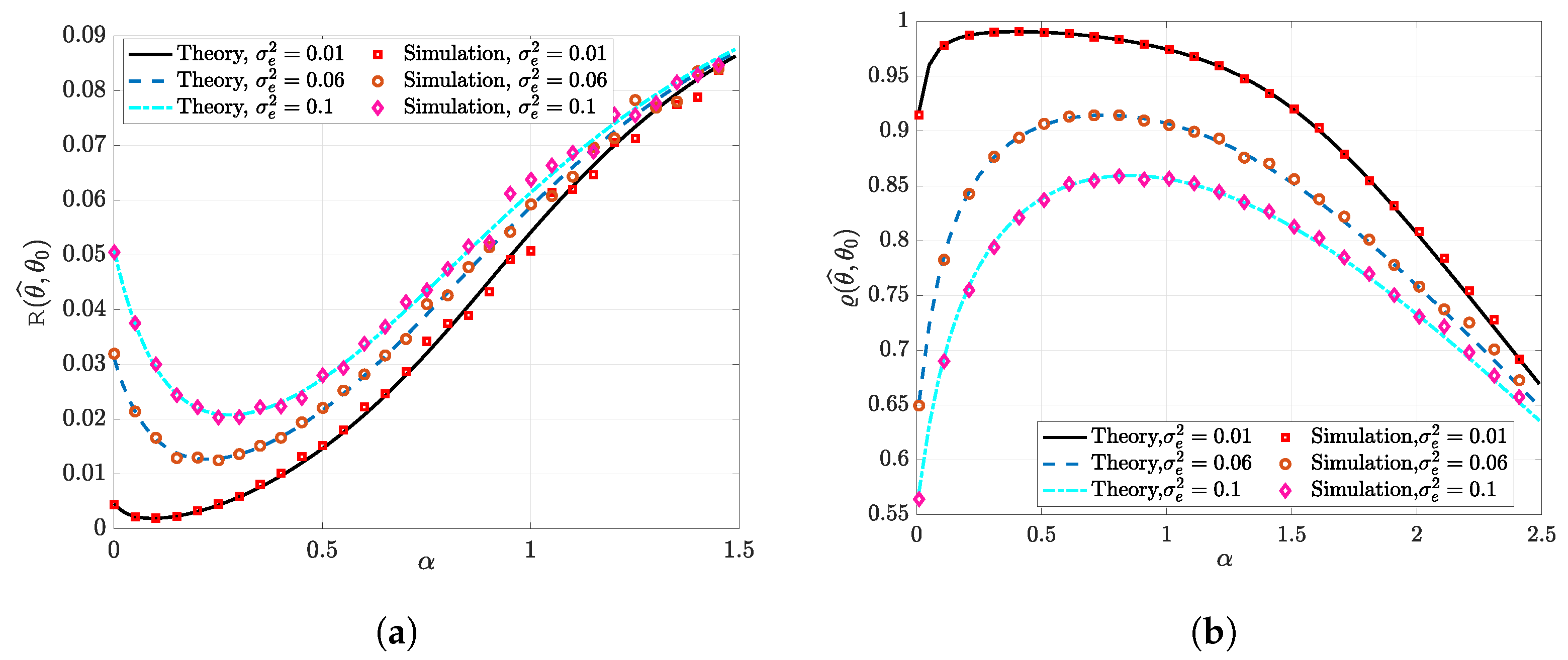
6. Additional Numerical Experiments

In this section, we provide additional numerical experiments to validate our results. These experiments are performed on synthetic data beyond the Gaussian ensemble and on real data as well. In addition, we empirically discuss the double descent phenomenon.

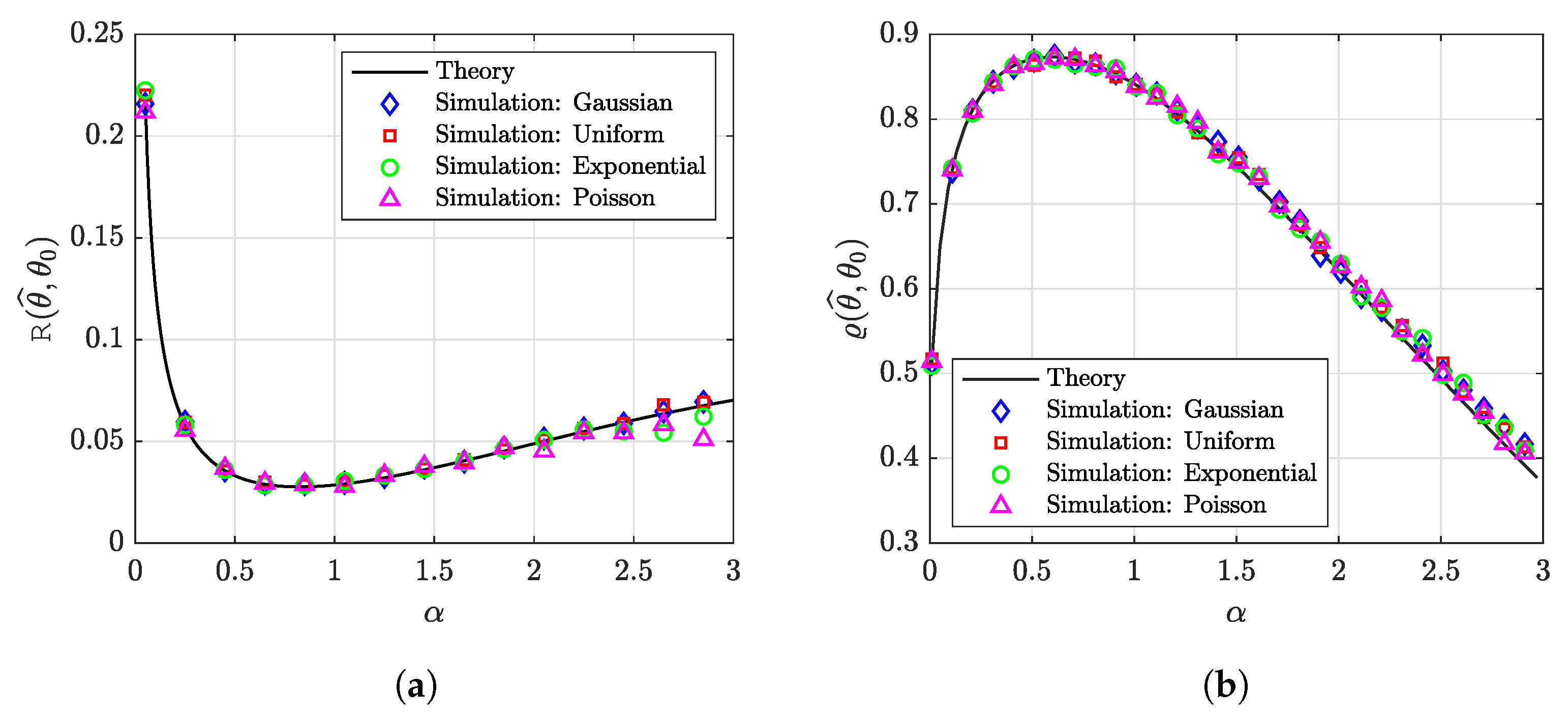
6.1. Synthetic Data: Universality of the Gaussian Design

Theorem 1 assumes that the elements of matrix X are i.i.d. Gaussian distributed. However, we expect the asymptotic results derived in this paper (prediction risk, similarity, etc.) to be robust and hold for a larger class of random matrices. Rigorous proofs are presented in [65,66,67,68,69], where the asymptotic prediction is shown to have a universal limit (as $p\to \infty$) with respect to random matrices with i.i.d. entries.

To validate the above claims, see Figure 8, where we plotted the prediction risk and the similarity for a sparse-Gaussian target vector with i.i.d. entries that follow the distribution: ${\theta }_{0,j}\sim (1-\rho ){\delta }_0+\rho \mathsf{N}(0,2)$. We used the G-PCR with an ${\mathcal{l}}_1$-norm in (18) to obtain the estimates. In addition to the Gaussian design matrix, we simulated the performance using other random matrices with i.i.d. entries drawn from a uniform distribution $\sqrt{\frac{3}{p}}\mathcal{U}[-1,1]$, an exponential distribution $\frac{1}{\sqrt{p}}\mathrm{Exp}\left(1\right)$, and from a Poisson distribution $\frac{1}{\sqrt{p}}\mathrm{Poiss}\left(1\right)$. Note that the normalization of these matrices is used to satisfy the high-dimensionality assumptions in Section 2.2. From this figure, we can see that the behavior seems to be nearly identical for all distributions, suggesting that our results enjoy a universality property.

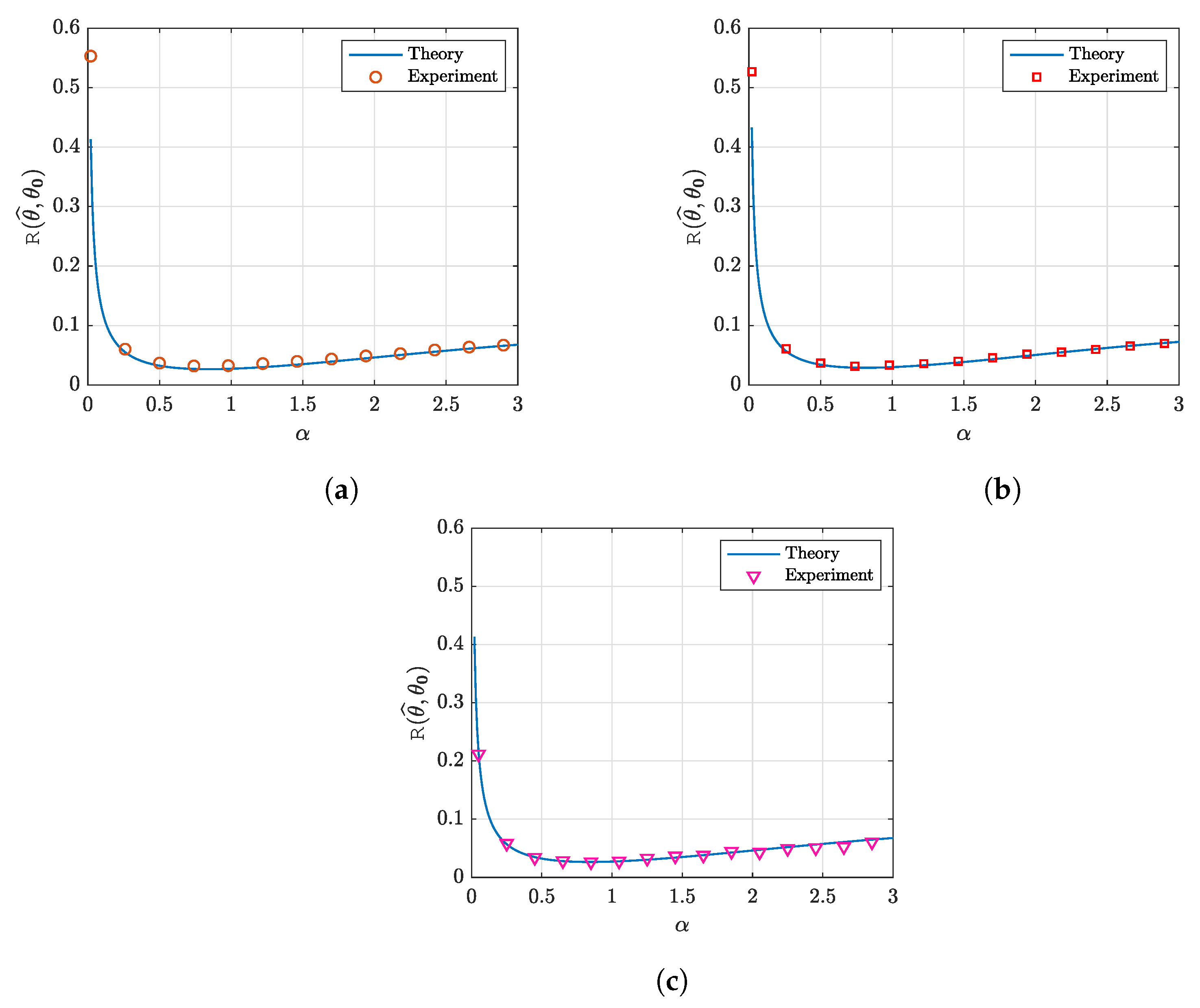
6.2. Real-World Data

In previous section, we showed the robustness of our results to the distribution of the i.i.d. entries of the data matrix $\mathbf{X}$. In this section, we take it a step further and consider real-world datasets instead of the synthetic data discussed earlier. These datasets are essentially not random and do not have i.i.d. elements. However, as seen in the numerical simulations below, they match our theoretical results to a great extent.

As an illustration, we present in Figure 9 the outcomes of these simulations for three real datasets. Each of these datasets consists of a small number of samples (n) and a high-dimensional feature space (p), which is consistent with the over-parameterized setting ($p>n$). These datasets are mainly for detecting several diseases and cancer samples. We generated the target vector, ${\mathit{\theta }}_0$, randomly with entries following the distribution ${\theta }_{0,j}\sim (1-\rho ){\delta }_0+\rho \mathsf{N}(0,1)$. The noise vector ϵ was generated using i.i.d. $\mathsf{N}(0,0.2)$ elements. We generated the observations as $\mathbf{y}=\mathbf{X}{\mathit{\theta }}_0+\mathit{ϵ}$. The G-PCR with ${\mathcal{l}}_1$-norm penalty in (18) is used to obtain $\widehat{\mathit{\theta }}$ with $\widehat{\mathbf{X}}=\mathbf{X}+\mathbf{E}$.

The three figures correspond to the following datasets:

• Figure 9a: For this figure, we used breast cancer data [70] (available at: https://github.com/kivancguckiran/microarray-data (accessed on 27 May 2023)). This dataset has been used in [71] for DNA microarray gene expression classification using the LASSO. It consists of 22,215 gene expressions (features) and 118 samples. From this matrix, we took a sub-matrix X of aspect ratio $\zeta =0.75$. We standardized all columns of matrix X to have mean 0 and variance 1.
• Figure 9b: In this figure, glioma disease data [72] were used (available at: https://github.com/kivancguckiran/microarray-data (accessed on 27 May 2023)). This dataset includes 54,613 features and 180 samples. Similar to the breast cancer data, the sub-matrix X with the same aspect ratio $\zeta$ was selected and standardized.
• Figure 9c: The dataset used in this figure includes colon cancer data [73] (available at: http://www.weizmann.ac.il/mcb/UriAlon/download/downloadable-data (accessed on 27 May 2023)). This dataset was used in [74] for a sparse-group LASSO model. It includes 2000 genes and 62 samples (22 normal tissues and 40 colon tumor tissues). Similar to the previous datasets, we selected a sub-matrix X with aspect ratio $\zeta$ and standardized it.

For all figures, we can see that the agreement between theory and simulations is remarkably good.

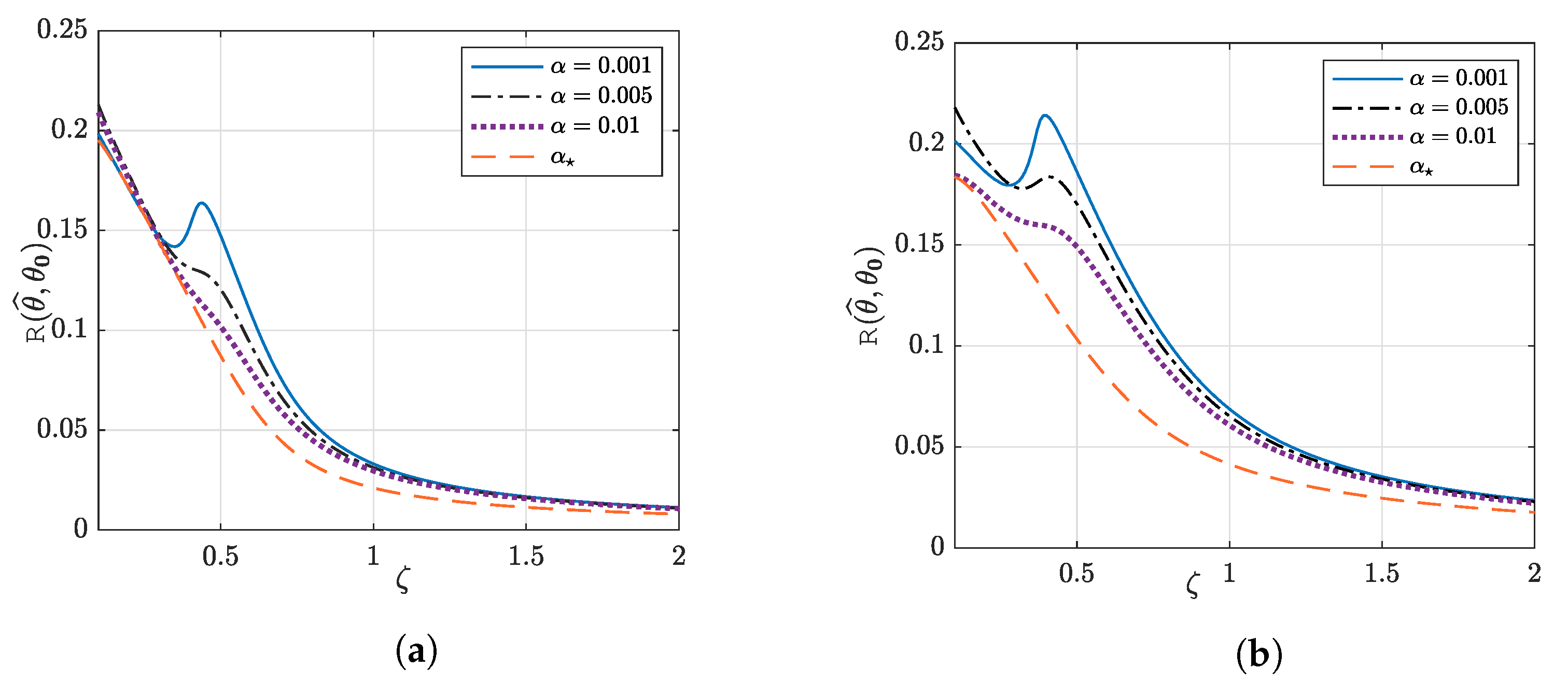
6.3. Double Descent Phenomenon

In Figure 10, we plotted the prediction risk as a function of $\zeta$ for different choices of the penalization factor $\alpha$. As can be seen, for an arbitrary choice of $\alpha$, the prediction risk of the G-PCR first decreases for small values of $\zeta$, then increases until it reaches a peak known as the interpolation peak. After that, the prediction risk decreases monotonically with respect to $\zeta$. This is known as the double descent phenomenon [75]. On the other hand, optimal values of the penalization factor ${\alpha }_{★}$ always guarantee that the prediction risk decreases with more training samples being used (i.e., with increasing $\zeta$). This emphasizes the important role of the optimal tuning of $\alpha$ to mitigate the double descent phenomenon and to give the best performance.

7. Conclusions

In this paper, we studied the high-dimensional error performance of the generalized penalized constrained regression (G-PCR) optimization with noisy features. Several analytical expressions were derived to measure the performance, such as the prediction risk, similarity, probability of misdetection, and probability of false alarm. Different popular instances of this optimization, such as ${\mathcal{l}}_1$-norm penalized regression and ${\mathcal{l}}_2$-norm penalization, were considered. We presented numerical simulations to validate these expressions based on both synthetic and real data. These results can be used to tune the involved hyper-parameters efficiently.

Furthermore, we empirically investigated the so-called double descent phenomenon and showed that optimal penalization can mitigate its effect. We also illustrated through several simulations the universality of our results beyond the assumed Gaussian distribution.

Finally, we note that numerical simulations have shown that our rigorous results are accurate even for problems with a few hundred variables, despite the fact that these results are assumed to be asymptotic in the problem dimensions.

References

1. Parikh, N.; Boyd, S. Proximal algorithms. Found. Trends Optim. 2014, 1, 127–239. [Google Scholar] [CrossRef]
2. Tarantola, A. Inverse Problem Theory and Methods for Model Parameter Estimation; SIAM: Philadelphia, PA, USA, 2005. [Google Scholar]
3. Kailath, T.; Sayed, A.H.; Hassibi, B. Linear Estimation; Prentice Hall: Hoboken, NJ, USA, 2000. [Google Scholar]
4. Groetsch, C.W.; Groetsch, C. Inverse Problems in the Mathematical Sciences; Springer: Berlin/Heidelberg, Germany, 1993; Volume 52. [Google Scholar]
5. Bishop, C.M. Pattern recognition. Mach. Learn. 2006, 128, 1–58. [Google Scholar]
6. Rencher, A.C.; Schaalje, G.B. Linear Models in Statistics; John Wiley & Sons: Hoboken, NJ, USA, 2008. [Google Scholar]
7. Dhar, V. Data science and prediction. Commun. ACM 2013, 56, 64–73. [Google Scholar] [CrossRef]
8. Donoho, D.L. Compressed sensing. IEEE Trans. Inf. Theory 2006, 52, 1289–1306. [Google Scholar] [CrossRef]
9. Duarte, M.F.; Eldar, Y.C. Structured compressed sensing: From theory to applications. IEEE Trans. Signal Process. 2011, 59, 4053–4085. [Google Scholar] [CrossRef]
10. Poor, H.V. An Introduction to Signal Detection and Estimation; Springer Science & Business Media: Berlin/Heidelberg, Germany, 1998. [Google Scholar]
11. Fadili, J.M.; Bullmore, E. Penalized partially linear models using sparse representations with an application to fMRI time series. IEEE Trans. Signal Process. 2005, 53, 3436–3448. [Google Scholar] [CrossRef]
12. Goldsmith, A. Wireless Communications; Cambridge University Press: Cambridge, UK, 2005. [Google Scholar]
13. Marzetta, T.L.; Yang, H. Fundamentals of Massive MIMO; Cambridge University Press: Cambridge, UK, 2016. [Google Scholar]
14. Candes, E.; Tao, T. The Dantzig selector: Statistical estimation when p is much larger than n. Ann. Stat. 2007, 35, 2313–2351. [Google Scholar]
15. Bach, F. Structured sparsity-inducing norms through submodular functions. In Proceedings of the Advances in Neural Information Processing Systems, Vancouver, BC, Canada, 6–9 December 2010; Volume 23. [Google Scholar]
16. Aster, R.C.; Borchers, B.; Thurber, C.H. Parameter Estimation and Inverse Problems; Elsevier: Amsterdam, The Netherlands, 2018. [Google Scholar]
17. McDonald, G.C. Ridge regression. Wiley Interdiscip. Rev. Comput. Stat. 2009, 1, 93–100. [Google Scholar] [CrossRef]
18. Tibshirani, R. Regression shrinkage and selection via the lasso. J. R. Stat. Soc. Ser. B 1996, 58, 267–288. [Google Scholar] [CrossRef]
19. Varah, J.M. Pitfalls in the numerical solution of linear ill-posed problems. SIAM J. Sci. Stat. Comput. 1983, 4, 164–176. [Google Scholar] [CrossRef]
20. Thrampoulidis, C.; Abbasi, E.; Hassibi, B. Precise error analysis of regularized M-estimators in high dimensions. IEEE Trans. Inf. Theory 2018, 64, 5592–5628. [Google Scholar] [CrossRef]
21. Bickel, P.J.; Ritov, Y.; Tsybakov, A.B. Simultaneous analysis of Lasso and Dantzig selector. Ann. Stat. 2009, 37, 1705–1732. [Google Scholar] [CrossRef]
22. Negahban, S.; Yu, B.; Wainwright, M.J.; Ravikumar, P.K. A unified framework for high-dimensional analysis of m-estimators with decomposable regularizers. In Proceedings of the Advances in Neural Information Processing Systems, Vancouver, BC, Canada, 7–10 December 2009; pp. 1348–1356. [Google Scholar]
23. Wainwright, M.J. Sharp thresholds for high-dimensional and noisy sparsity recovery using -constrained quadratic programming (Lasso). IEEE Trans. Inf. Theory 2009, 55, 2183–2202. [Google Scholar] [CrossRef]
24. Belloni, A.; Chernozhukov, V.; Wang, L. Square-root lasso: Pivotal recovery of sparse signals via conic programming. Biometrika 2011, 98, 791–806. [Google Scholar] [CrossRef]
25. Li, Y.H.; Hsieh, Y.P.; Zerbib, N.; Cevher, V. A geometric view on constrained M-estimators. arXiv 2015, arXiv:1506.08163. [Google Scholar]
26. Bayati, M.; Montanari, A. The dynamics of message passing on dense graphs, with applications to compressed sensing. IEEE Trans. Inf. Theory 2011, 57, 764–785. [Google Scholar] [CrossRef]
27. Bayati, M.; Montanari, A. The LASSO risk for Gaussian matrices. IEEE Trans. Inf. Theory 2012, 58, 1997–2017. [Google Scholar] [CrossRef]
28. Donoho, D.; Montanari, A. High dimensional robust m-estimation: Asymptotic variance via approximate message passing. Probab. Theory Relat. Fields 2016, 166, 935–969. [Google Scholar] [CrossRef]
29. Rangan, S.; Goyal, V.; Fletcher, A.K. Asymptotic analysis of map estimation via the replica method and compressed sensing. In Proceedings of the Advances in Neural Information Processing Systems, Vancouver, BC, Canada, 7–10 December 2009; Volume 22. [Google Scholar]
30. Kabashima, Y.; Wadayama, T.; Tanaka, T. Statistical mechanical analysis of a typical reconstruction limit of compressed sensing. In Proceedings of the 2010 IEEE International Symposium on Information Theory, Austin, TX, USA, 13–18 June 2010; IEEE: Piscataway, NJ, USA, 2010; pp. 1533–1537. [Google Scholar]
31. Couillet, R.; Debbah, M. Random Matrix Methods for Wireless Communications; Cambridge University Press: Cambridge, UK, 2011. [Google Scholar]
32. Karoui, N.E. Asymptotic behavior of unregularized and ridge-regularized high-dimensional robust regression estimators: Rigorous results. arXiv 2013, arXiv:1311.2445. [Google Scholar]
33. Liao, Z.; Couillet, R. Random matrices meet machine learning: A large dimensional analysis of ls-svm. In Proceedings of the 2017 IEEE International Conference on Acoustics, Speech and Signal Processing (ICASSP), New Orleans, LA, USA, 5–9 March 2017; IEEE: Piscataway, NJ, USA, 2017; pp. 2397–2401. [Google Scholar]
34. El Karoui, N. On the impact of predictor geometry on the performance on high-dimensional ridge-regularized generalized robust regression estimators. Probab. Theory Relat. Fields 2018, 170, 95–175. [Google Scholar] [CrossRef]
35. Stojnic, M. Recovery thresholds for 1 optimization in binary compressed sensing. In Proceedings of the 2010 IEEE International Symposium on Information Theory, Austin, TX, USA, 13–18 June 2010; IEEE: Piscataway, NJ, USA, 2010; pp. 1593–1597. [Google Scholar]
36. Stojnic, M. A framework to characterize performance of lasso algorithms. arXiv 2013, arXiv:1303.7291. [Google Scholar]
37. Thrampoulidis, C.; Oymak, S.; Hassibi, B. Regularized Linear Regression: A Precise Analysis of the Estimation Error. In Proceedings of the COLT, Paris, France, 3–6 July 2015; pp. 1683–1709. [Google Scholar]
38. Thrampoulidis, C.; Panahi, A.; Guo, D.; Hassibi, B. Precise error analysis of the lasso. In Proceedings of the 2015 IEEE International Conference on Acoustics, Speech and Signal Processing (ICASSP), South Brisbane, Australia, 19–24 April 2015; IEEE: Piscataway, NJ, USA, 2015; pp. 3467–3471. [Google Scholar]
39. Thrampoulidis, C.; Xu, W.; Hassibi, B. Symbol error rate performance of box-relaxation decoders in massive MIMO. IEEE Trans. Signal Process. 2018, 66, 3377–3392. [Google Scholar] [CrossRef]
40. Atitallah, I.B.; Thrampoulidis, C.; Kammoun, A.; Al-Naffouri, T.Y.; Hassibi, B.; Alouini, M.S. Ber analysis of regularized least squares for bpsk recovery. In Proceedings of the 2017 IEEE International Conference on Acoustics, Speech and Signal Processing (ICASSP), New Orleans, LA, USA, 5–9 March 2017; IEEE: Piscataway, NJ, USA, 2017; pp. 4262–4266. [Google Scholar]
41. Alrashdi, A.M.; Kammoun, A.; Muqaibel, A.H.; Al-Naffouri, T.Y. Asymptotic Performance of Box-RLS Decoders under Imperfect CSI with Optimized Resource Allocation. IEEE Open J. Commun. Soc. 2022, 3, 2051–2075. [Google Scholar] [CrossRef]
42. Atitallah, I.B.; Thrampoulidis, C.; Kammoun, A.; Al-Naffouri, T.Y.; Alouini, M.S.; Hassibi, B. The BOX-LASSO with application to GSSK modulation in massive MIMO systems. In Proceedings of the 2017 IEEE International Symposium on Information Theory (ISIT), Aachen, Germany, 25–30 June 2017; IEEE: Piscataway, NJ, USA, 2017; pp. 1082–1086. [Google Scholar]
43. Alrashdi, A.M.; Alrashdi, A.E.; Alghadhban, A.; Eleiwa, M.A. Optimum GSSK Transmission in Massive MIMO Systems Using the Box-LASSO Decoder. IEEE Access 2022, 10, 15845–15859. [Google Scholar] [CrossRef]
44. Alrashdi, A.M.; Atitallah, I.B.; Al-Naffouri, T.Y. Precise performance analysis of the box-elastic net under matrix uncertainties. IEEE Signal Process. Lett. 2019, 26, 655–659. [Google Scholar] [CrossRef]
45. Hayakawa, R.; Hayashi, K. Binary vector reconstruction via discreteness-aware approximate message passing. In Proceedings of the 2017 Asia-Pacific Signal and Information Processing Association Annual Summit and Conference (APSIPA ASC), Kuala Lumpur, Malaysia, 12–15 December 2017; IEEE: Piscataway, NJ, USA, 2017; pp. 1783–1789. [Google Scholar]
46. Hayakawa, R.; Hayashi, K. Asymptotic Performance of Discrete-Valued Vector Reconstruction via Box-Constrained Optimization With Sum of 1 Regularizers. IEEE Trans. Signal Process. 2020, 68, 4320–4335. [Google Scholar] [CrossRef]
47. Deng, Z.; Kammoun, A.; Thrampoulidis, C. A model of double descent for high-dimensional binary linear classification. Inf. Inference J. IMA 2022, 11, 435–495. [Google Scholar] [CrossRef]
48. Kini, G.R.; Thrampoulidis, C. Analytic study of double descent in binary classification: The impact of loss. In Proceedings of the 2020 IEEE International Symposium on Information Theory (ISIT), Los Angeles, CA, USA, 21–26 June 2020; IEEE: Piscataway, NJ, USA, 2020; pp. 2527–2532. [Google Scholar]
49. Salehi, F.; Abbasi, E.; Hassibi, B. The performance analysis of generalized margin maximizers on separable data. In Proceedings of the International Conference on Machine Learning, Virtual Online, 13–18 July 2020; PMLR: Mc Kees Rocks, PA, USA, 2020; pp. 8417–8426. [Google Scholar]
50. Dhifallah, O.; Thrampoulidis, C.; Lu, Y.M. Phase retrieval via linear programming: Fundamental limits and algorithmic improvements. In Proceedings of the 2017 55th Annual Allerton Conference on Communication, Control, and Computing (Allerton), Monticello, IL, USA, 3–6 October 2017; IEEE: Piscataway, NJ, USA, 2017; pp. 1071–1077. [Google Scholar]
51. Salehi, F.; Abbasi, E.; Hassibi, B. A precise analysis of phasemax in phase retrieval. In Proceedings of the 2018 IEEE International Symposium on Information Theory (ISIT), Vail, CO, USA, 17–22 June 2018; IEEE: Piscataway, NJ, USA, 2018; pp. 976–980. [Google Scholar]
52. Bosch, D.; Panahi, A.; Hassibi, B. Precise Asymptotic Analysis of Deep Random Feature Models. arXiv 2023, arXiv:2302.06210. [Google Scholar]
53. Dhifallah, O.; Lu, Y.M. A precise performance analysis of learning with random features. arXiv 2020, arXiv:2008.11904. [Google Scholar]
54. Dhifallah, O.; Lu, Y.M. Phase transitions in transfer learning for high-dimensional perceptrons. Entropy 2021, 23, 400. [Google Scholar] [CrossRef]
55. Ting, M.; Raich, R.; Hero, A.O., III. Sparse image reconstruction for molecular imaging. IEEE Trans. Image Process. 2009, 18, 1215–1227. [Google Scholar] [CrossRef]
56. Gui, G.; Peng, W.; Wang, L. Improved sparse channel estimation for cooperative communication systems. Int. J. Antennas Propag. 2012, 2012, 476509. [Google Scholar] [CrossRef]
57. Luenberger, D.G.; Ye, Y. Linear and Nonlinear Programming; Springer: Berlin/Heidelberg, Germany, 1984; Volume 2. [Google Scholar]
58. Salehi, F.; Abbasi, E.; Hassibi, B. The impact of regularization on high-dimensional logistic regression. In Proceedings of the Advances in Neural Information Processing Systems, Vancouver, BC, Canada, 8–14 December 2019; Volume 32. [Google Scholar]
59. Donoho, D.L.; Maleki, A.; Montanari, A. Message-passing algorithms for compressed sensing. Proc. Natl. Acad. Sci. USA 2009, 106, 18914–18919. [Google Scholar] [CrossRef]
60. Hayakawa, R. Noise variance estimation using asymptotic residual in compressed sensing. arXiv 2020, arXiv:2009.13678. [Google Scholar]
61. Suliman, M.A.; Alrashdi, A.M.; Ballal, T.; Al-Naffouri, T.Y. SNR estimation in linear systems with Gaussian matrices. IEEE Signal Process. Lett. 2017, 24, 1867–1871. [Google Scholar] [CrossRef]
62. Kobayashi, H.; Mark, B.L.; Turin, W. Probability, Random Processes, and Statistical Analysis: Applications to Communications, Signal Processing, Queueing Theory and Mathematical Finance; Cambridge University Press: Cambridge, UK, 2011. [Google Scholar]
63. Donoho, D.L.; Maleki, A.; Montanari, A. The noise-sensitivity phase transition in compressed sensing. IEEE Trans. Inf. Theory 2011, 57, 6920–6941. [Google Scholar] [CrossRef]
64. Thrampoulidis, C.; Abbasi, E.; Hassibi, B. Lasso with non-linear measurements is equivalent to one with linear measurements. In Proceedings of the Advances in Neural Information Processing Systems, Montreal, QC, USA, 7–12 December 2015; pp. 3420–3428. [Google Scholar]
65. Abbasi, E.; Salehi, F.; Hassibi, B. Universality in learning from linear measurements. In Proceedings of the Advances in Neural Information Processing Systems, Vancouver, BC, Canada, 8–14 December 2019; Volume 32. [Google Scholar]
66. Hu, H.; Lu, Y.M. Universality laws for high-dimensional learning with random features. IEEE Trans. Inf. Theory 2022, 69, 1932–1964. [Google Scholar] [CrossRef]
67. Han, Q.; Shen, Y. Universality of regularized regression estimators in high dimensions. arXiv 2022, arXiv:2206.07936. [Google Scholar]
68. Dudeja, R.; Bakhshizadeh, M. Universality of linearized message passing for phase retrieval with structured sensing matrices. IEEE Trans. Inf. Theory 2022, 68, 7545–7574. [Google Scholar] [CrossRef]
69. Gerace, F.; Krzakala, F.; Loureiro, B.; Stephan, L.; Zdeborová, L. Gaussian Universality of Perceptrons with Random Labels. arXiv 2023, arXiv:2205.13303. [Google Scholar]
70. Chin, K.; DeVries, S.; Fridlyand, J.; Spellman, P.T.; Roydasgupta, R.; Kuo, W.L.; Lapuk, A.; Neve, R.M.; Qian, Z.; Ryder, T.; et al. Genomic and transcriptional aberrations linked to breast cancer pathophysiologies. Cancer Cell 2006, 10, 529–541. [Google Scholar] [CrossRef]
71. Güçkiran, K.; Cantürk, İ.; Özyilmaz, L. DNA microarray gene expression data classification using SVM, MLP, and RF with feature selection methods relief and LASSO. Süleyman Demirel Üniv. Fen Bilim. Enstitüsü Derg. 2019, 23, 126–132. [Google Scholar] [CrossRef]
72. Sun, L.; Hui, A.M.; Su, Q.; Vortmeyer, A.; Kotliarov, Y.; Pastorino, S.; Passaniti, A.; Menon, J.; Walling, J.; Bailey, R.; et al. Neuronal and glioma-derived stem cell factor induces angiogenesis within the brain. Cancer Cell 2006, 9, 287–300. [Google Scholar] [CrossRef]
73. Alon, U.; Barkai, N.; Notterman, D.A.; Gish, K.; Ybarra, S.; Mack, D.; Levine, A.J. Broad patterns of gene expression revealed by clustering analysis of tumor and normal colon tissues probed by oligonucleotide arrays. Proc. Natl. Acad. Sci. USA 1999, 96, 6745–6750. [Google Scholar] [CrossRef] [PubMed]
74. Li, J.; Dong, W.; Meng, D. Grouped gene selection of cancer via adaptive sparse group lasso based on conditional mutual information. IEEE/ACM Trans. Comput. Biol. Bioinform. 2017, 15, 2028–2038. [Google Scholar] [CrossRef] [PubMed]
75. Belkin, M.; Hsu, D.; Ma, S.; Mandal, S. Reconciling modern machine-learning practice and the classical bias—Variance trade-off. Proc. Natl. Acad. Sci. USA 2019, 116, 15849–15854. [Google Scholar] [CrossRef] [PubMed]
76. Gordon, Y. On Milman’s inequality and random subspaces which escape through a mesh in n. In Geometric Aspects of Functional Analysis; Lecture Notes in Mathematics; Springer: Berlin/Heidelberg, Germany, 1988; pp. 84–106. [Google Scholar]
77. Chu, H.T.; Toh, K.C.; Zhang, Y. On Regularized Square-root Regression Problems: Distributionally Robust Interpretation and Fast Computations. J. Mach. Learn. Res. 2022, 23, 13885–13923. [Google Scholar]
78. Bunea, F.; Lederer, J.; She, Y. The group square-root lasso: Theoretical properties and fast algorithms. IEEE Trans. Inf. Theory 2013, 60, 1313–1325. [Google Scholar] [CrossRef]
Figure 1. A system model comparison between the original G-PCR recovery algorithm and its scalar decoupled version. (a) Original system. (b) Scalar decoupled system.
Mathematics 11 03706 g001
Figure 2. Performance of the G-PCR vs. the penalization factor for a sparse linear regression. The parameters are set as follows: p = 300 , ζ = 1.5 , ρ = 0.2 , σ ϵ 2 = 0.1 , L = 1 , and U = 1 . The simulation results are averaged over 50 independent Monte Carlo trials. (a) The prediction risk. (b) The cosine similarity.
Mathematics 11 03706 g002
Figure 3. Performance comparison between the G-PCR and G-PR. For the numerical simulations, the results are averaged over 100 independent trials, with p = 128 , ζ = 0.85 , ρ = 0.1 , σ ϵ 2 = 0.2 , σ e 2 = 0.05 , L = 1 , and U = 1 . (a) The prediction risk. (b) The cosine similarity.
Mathematics 11 03706 g003
Figure 4. Probability mass function (PMF) of a sparse-binary distribution.
Mathematics 11 03706 g004
Figure 5. Support recovery performance of the G-PCR versus the penalization factor for a sparse-binary signal recovery. The parameters are set as follows: E = 1 , p = 300 , ζ = 0.85 , ρ = 0.2 , σ ϵ 2 = 0.05 , ξ = 0.1 , L = 0 , and U = 1 . The simulations are averaged over 100 independent Monte Carlo trials. (a) Probability of misdetection. (b) Probability of false alarm.
Mathematics 11 03706 g005
Figure 6. Performance of the l 2 2 -norm G-PCR vs. the penalization factor for a Gaussian target vector. The parameters are set as follows: p = 500 , ζ = 1.3 , σ θ 2 = 1 , σ e 2 = 0.01 , σ ϵ 2 = 0.01 , L = 1 , and U = 1 . The results are averaged over 50 independent realizations. (a) The prediction risk. (b) The cosine similarity.
Mathematics 11 03706 g006
Figure 7. Classification error rate ( C err ) of the G-PCR vs.the penalization factor for a binary target vector. The parameters are set as follows: p = 500 , ζ = 0.85 , σ e 2 = 0.01 , σ ϵ 2 = 0.02 , and L = U = 1 . The results are averaged over 100 independent Monte Carlo trials.
Mathematics 11 03706 g007
Figure 8. Performance the G-PCR for a sparse-Gaussian target vector. We set the parameters as p = 180 , ζ = 0.95 , σ e 2 = 0.1 , σ ϵ 2 = 0.2 , ρ = 0.1 , and L = U = 2 . The results are averaged over 50 independent trials. (a) The prediction risk. (b) The similarity.
Mathematics 11 03706 g008
Figure 9. Prediction risk as a function of the penalization factor α . Here, the data matrix X is a standardized real dataset. We used a sparse-Gaussian vector θ 0 , and we generated the observations as y = X θ 0 + ϵ . The G-PCR with l 1 -norm penalty is used to obtain θ ^ with X ^ = X + E . The parameters are set as ζ = 0.75 , ρ = 0.1 , σ ϵ 2 = 0.2 , σ e 2 = 0.1 , and L = U = 1 . The results are averaged over 200 independent trials. (a) Breast cancer data. (b) Glioma disease data. (c) Colon cancer data.
Mathematics 11 03706 g009
Figure 10. Prediction risk as a function of the aspect ratio ζ . We used G-PCR with an l 1 -norm penalty and sparse-binary vector with ρ = 0.2 , σ e 2 = 0.1 , L = 0 , and U = 1 . (a) σ ϵ 2 = 0.1 . (b) σ ϵ 2 = 0.3 . Illustration of the double descent and how optimal penalization can mitigate it.
Mathematics 11 03706 g010
Disclaimer/Publisher’s Note: The statements, opinions and data contained in all publications are solely those of the individual author(s) and contributor(s) and not of MDPI and/or the editor(s). MDPI and/or the editor(s) disclaim responsibility for any injury to people or property resulting from any ideas, methods, instructions or products referred to in the content.