Article

Numerical Solution of Transition to Turbulence over Compressible Ramp at Hypersonic Velocity

Department of Technical Mathematics, Faculty of Mechanical Engineering, CTU in Prague, 16636 Prague, Czech Republic
Current address: Karlovo náměstí 13, 121 35 Praha 2, 16636 Prague, Czech Republic.
Mathematics 2023, 11(17), 3684; https://doi.org/10.3390/math11173684
Submission received: 31 July 2023 / Revised: 20 August 2023 / Accepted: 22 August 2023 / Published: 26 August 2023
(This article belongs to the Special Issue Mathematical Dynamic Flow Models)

Abstract

:
This work deals with the numerical solution of hypersonic flow of viscous fluid over a compressible ramp. The solved case involves very important and complicated phenomena such as the interaction of the shock wave with the boundary layer or the transition from a laminar to a turbulent state. This type of problem is very important as it is often found on re-entry vehicles, engine intakes, system and sub-system junctions, etc. Turbulent flow is modeled by the system of averaged Navier–Stokes equations, which is completed by the explicit algebraic model of Reynolds stresses (EARSM model) and further enhanced by the algebraic model of bypass transition. The numerical solution is obtained by the finite volume method based on the rotated-hybrid Riemann solver and explicit multistage Runge–Kutta method. The numerical solution is then compared with the results of a direct numerical simulation.

1. Introduction

The design of hypersonic vehicles is becoming increasingly common nowadays, and it is therefore necessary to develop and use appropriate engineering tools.
Hypersonic flow has a very complex nature. Strong shock waves may be present in the flow field as well as in their interactions with each other or with the boundary layer. Contact waves, large areas of a subsonic flow field, supersonic jets, and other complicated elements may also be present in the flow field. Measuring these flow fields in experimental aerodynamic laboratories can be technically difficult and expensive. Therefore, computational fluid dynamics (CFD) methods are increasingly being used.
Solving hypersonic flow using CFD methods is still a major challenge. It is necessary to use a suitable numerical method that is sufficiently robust, stable, and capable of approximating the flow at low and high Mach numbers. The numerical scheme must also be able to accurately capture all the flow field elements described above. Recent developments in numerical methods, e.g., [1,2,3,4,5], address some of these problems.
Another issue is the appropriate modeling of turbulence, which is still an open problem. Many commonly used models of turbulence neglect terms that may only be significant at hypersonic velocities [6]. A significant part of the problem is modeling the transition from a laminar to a turbulent flow regime. The answer to all these problems may be the use of the direct numerical simulation (DNS), which can accurately predict hypersonic turbulent flows, e.g., [7,8,9,10]. However, the DNS method requires a very precise numerical method and a very fine computational mesh (the number of cells required for the DNS method is equal to R e 9 4 [6]). Therefore, its use for industrial applications in current computers is not possible.
The main objective of this work is to test the possibility of using a relatively common CFD method based on averaged Navier–Stokes equations closed by the modified EARSM model of turbulence and second-order accurate numerical method for hypersonic flow prediction.
The problem selected for this test is flow over a compressible ramp. Although the geometry of the problem is simple, the solution is complex and involves the interaction of shock waves, shock wave interaction with the boundary layer, and separation, reattachment, and even transition from a laminar to a turbulent state. This problem is the subject of current research, e.g., [7,11,12,13]. These publications use the DNS method, which is suitable for research purposes but very expensive for use in design calculations of re-entry vehicles or engine intakes, which are typical applications of solved problems.
The importance of this test is to determine whether common CFD methods can be used for such cases with sufficient accuracy for engineering designs.
The paper is organized as follows. First, the averaged Navier–Stokes equations together with the modified EARSM model of turbulence are introduced in Section 2. The following section deals with the numerical solution using the finite volume method. After that, the problem of flow over a compressible ramp is formulated and solved numerically. Finally, the obtained results are discussed in the last section.

2. Governing Equations

Turbulent flow of viscous compressible fluid is modeled by the system of averaged Navier–Stokes equations in vector form (summation over repeated indices will be used throughout the paper),
W t + F j ( W ) x j = R j ( W ) x j ,
F j ( W ) = ρ u j ρ u i u j + p δ i j ( ρ E + p ) u j , R j ( W ) = 0 τ i j + τ i j t u i ( τ i j + τ i j t ) ( q j + q j t ) + d j t ,
where W = ( ρ , ρ u i , ρ E ) T is the vector of mean conservative variables (Reynolds averaging is used for density and static pressure, and Favre averaging is used for total specific energy and for components of the velocity vector [14]), ρ is density, u i are components of the velocity vector, E is total specific energy, p is static pressure, and δ i j is the Kronecker delta. The components of the mean stress tensor τ i j are given by relation
τ i j = μ u i x j + u j x i 2 3 δ i j u k x k , μ = μ r e f ρ r e f p p r e f ρ 3 4 ,
where μ is the mean viscosity computed using the Rayleigh relation, with μ r e f , ρ r e f , and p r e f being constants. The components of the mean heat flux vector q j are defined as
q j = κ κ 1 μ P r x j p ρ ,
where κ is the specific heat ratio (in this work, the flow of perfect gas (air) is assumed, for which κ = 1.4 holds), and the Prandtl number P r is assumed to be constant (in this work, P r = 0.72 ). The components of the turbulent heat flux vector q j t are analogically ([6]) defined as
q j t = κ κ 1 μ t P r t x j p ρ ,
where the turbulent Prandtl number P r t is also assumed to be constant (in this work, P r t = 0.9 ). The term d t corresponds to the molecular diffusion and turbulent transport of the turbulent kinetic energy k. This term is usually neglected but can be significant in hypersonic flows [6]. The components d j t are given by the relation
d j t = ( μ + σ * μ t ) k x j .
The model constant σ * , the turbulent viscosity μ t , and components of the Reynolds stress tensor τ i j t will be given in the next subsection. The system of averaged Navier–Stokes Equations (1) is also equipped with the equation of state of a perfect gas in the form
p = ( κ 1 ) ρ E 1 2 ρ u j u j ρ k .

Model of Turbulence

The system of averaged Navier–Stokes Equations (1) is not closed and therefore needs to be completed by some suitable model of turbulence.
The model of turbulence used in this work is based on the EARSM model, which is further enhanced by the algebraic model of bypass transition [14].
The model consists of the transport equation for the turbulent kinetic energy k,
( ρ k ) t + ( ρ k u j ) x j = γ f S S P β * ρ k ω + x j μ + σ * μ t k x j ,
and transport equation for the specific dissipation rate ω ,
( ρ ω ) t + ( ρ ω u j ) x j = α ω k f S S P β ρ ω 2 + x j μ + σ μ t ω x j + C d ,
where
P = τ i j t u i x j
is the original production term of the turbulent kinetic energy [15], C d represents cross-diffusion given by the formula
C d = σ d ρ ω max k x j ω x j , 0 ,
and β * = 0.09 , σ * = 1.01 , α = 0.553 , β = 0.075 , σ = 0.5 , and σ d = 0.52 are model constants.
The algebraic model of bypass transition is represented by two functions, namely f S S and γ , where the first is sheer sheltering factor
f S S = exp C S S μ Ω ρ k 2 ,
where Ω = 2 Ω i j Ω i j is the vorticity tensor magnitude, and constant C S S = 2.75 . The latter function represents an intermittency factor defined as
γ = min ( max ( R e k Ω C T , 0 ) , 1 ) ,
where C T = 1.8125 is constant, and the Reynolds number R e k Ω , which serves as the transition onset parameter, is given by the relation
R e k Ω = ρ k μ Ω .
Finally, the last two terms in Equations (8) and (9) ( τ i j t and μ t ) are the components of the Reynolds stress tensor and turbulent viscosity, respectively. Both terms are parts of the EARSM model’s constitutive relations. The components of the Reynolds stress tensor are given as
τ i j t = μ t u i x j + u j x i 2 3 δ i j u k x k 2 3 δ i j ρ k ρ k a i j ( e x ) ,
where turbulent viscosity is given by the relation
μ t = 1 2 ( β 1 + II Ω β 6 ) ρ k τ ,
and extra anisotropy is given as
a i j ( e x ) = β 3 Ω i k * Ω k j * 1 3 II Ω δ i j + β 4 ( S i k * Ω k j * Ω i k * S k j * ) + β 6 S i k * Ω k l * Ω l j * + Ω i k * Ω k l * S l j * II Ω S i j * 2 3 IV δ i j + β 9 ( Ω i k * S k l * Ω l m * Ω m j * Ω i k * Ω k l * S l m * Ω m j * ) .
The turbulent viscosity μ t and extra anisotropy a i j ( e x ) are nonlinear terms, which depend on the turbulent time scale
τ = max 1 β * ω , 6 μ β * ρ k ω ,
dimensionless strain-rate and vorticity tensors
S i j * = τ 2 u i x j + u j x i 2 3 δ i j u k x k , Ω i j * = τ 2 u i x j u j x i ,
and on the related invariants II Ω = Ω k l * Ω l k * and IV = S k l * Ω l m * Ω m k * . The beta coefficients β 1 β 9 are defined as
β 1 = N ( 2 N 2 7 II Ω ) Q , β 3 = 12 N 1 IV Q ,
β 4 = 2 ( N 2 2 II Ω ) Q , β 6 = 6 N Q , β 9 = 6 Q ,
where the denominator Q is
Q = 5 6 ( N 2 2 II Ω ) ( 2 N 2 II Ω ) ,
with N representing the turbulent kinetic energy production and dissipation rate ratio defined as
N = N c + 162 IV 2 + ( V 0.5 II S II Ω ) N c 2 20 N c 4 ( N c 0.5 C 1 ) II Ω ( 10 N c 3 + 15 C 1 N c 2 ) + 10 C 1 II Ω 2 ,
where
N c = C 1 3 + P 1 + P 2 1 3 + sign P 1 P 2 | ( P 1 P 2 | 1 3 for P 2 0 C 1 3 + 2 P 1 2 P 2 1 6 cos 1 3 arccos P 1 P 1 2 P 2 for P 2 < 0 ,
P 1 = C 1 2 27 + 9 20 II S 2 3 II Ω C 1 , P 2 = P 1 2 C 1 2 9 + 9 10 II S + 2 3 II Ω 3 ,
II S = S k l * S l k * , V = S k l * S l m * Ω m n * Ω n k * ,
and C 1 is given by relation
C 1 = 9 5 + 9 4 C d i f f max 1 + β 1 e q II S , 0 ,
where
β 1 e q = 6 5 N e q ( N e q ) 2 2 II Ω , N e q = 81 20 and C diff = 2.2 .

3. Numerical Method

The system of averaged Navier–Stokes Equation (1), together with the transport equations of the EARSM model, can be written as
W t + F j ( W ) x j = R j ( W ) x j + Q ( W ) ,
where W = ( ρ , ρ u i , ρ E , ρ k , ρ ω ) T is the vector of the unknown conservative variables, F j are corresponding inviscid fluxes, R j are corresponding viscous fluxes, and vector Q contains source terms.
The numerical solution is obtained by in-house software based on the cell-centered finite volume method [16] in semi-discrete form
d W i d t = 1 | D i | k = 1 faces ( R ^ k F ^ k ) Δ S k + Q ( W i ) ,
where W i is an averaged solution over the cell D i , viscous flux R ^ = R · n , inviscid flux F ^ = F · n , Δ S is the area of the cell face between two adjacent cells, and n is the unit vector normal to a face.
Since hypersonic flow is considered in this work, a rotated-hybrid Riemann solver [1] is used for approximation of inviscid flux. By using the rotated-hybrid Riemann solver concept, a carbuncle phenomenon caused by strong shock waves can be avoided. Moreover, the rotated-hybrid Riemann solver is based on a combination of the low Mach number variants of the HLLC and the HLL schemes, respectively, which is important for accurate prediction of subsonic parts of the flow field.
Second-order accuracy is accomplished by piece-wise linear WENO reconstruction [17] of the primitive variables. The viscous flux is discretized by the central scheme with aid of diamond-shape dual cells [18]. Time integration of the semi-discrete finite volume method (30) is done by the explicit two-stage TVD Runge–Kutta method [19] with point implicit treatment of the source terms.

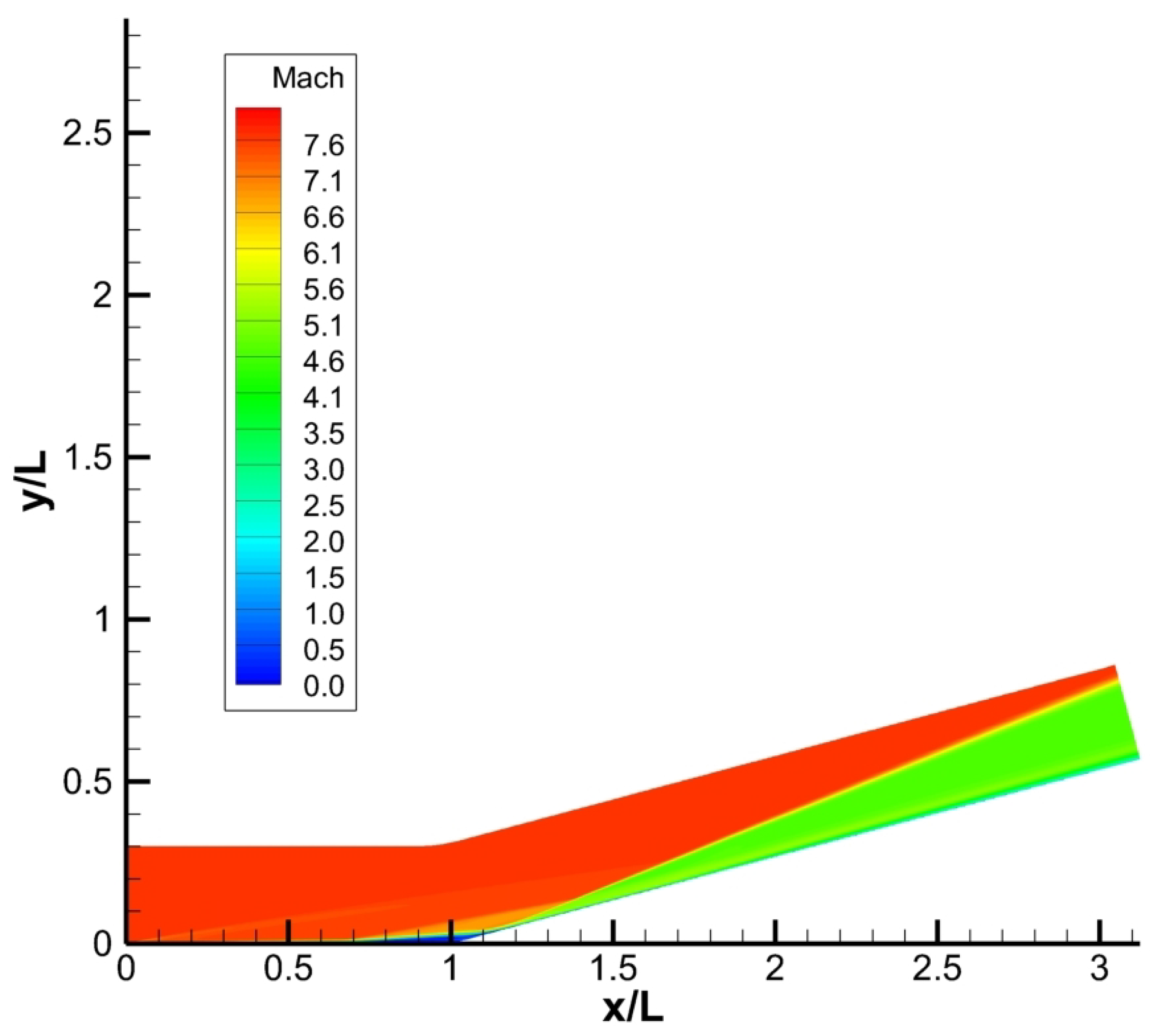
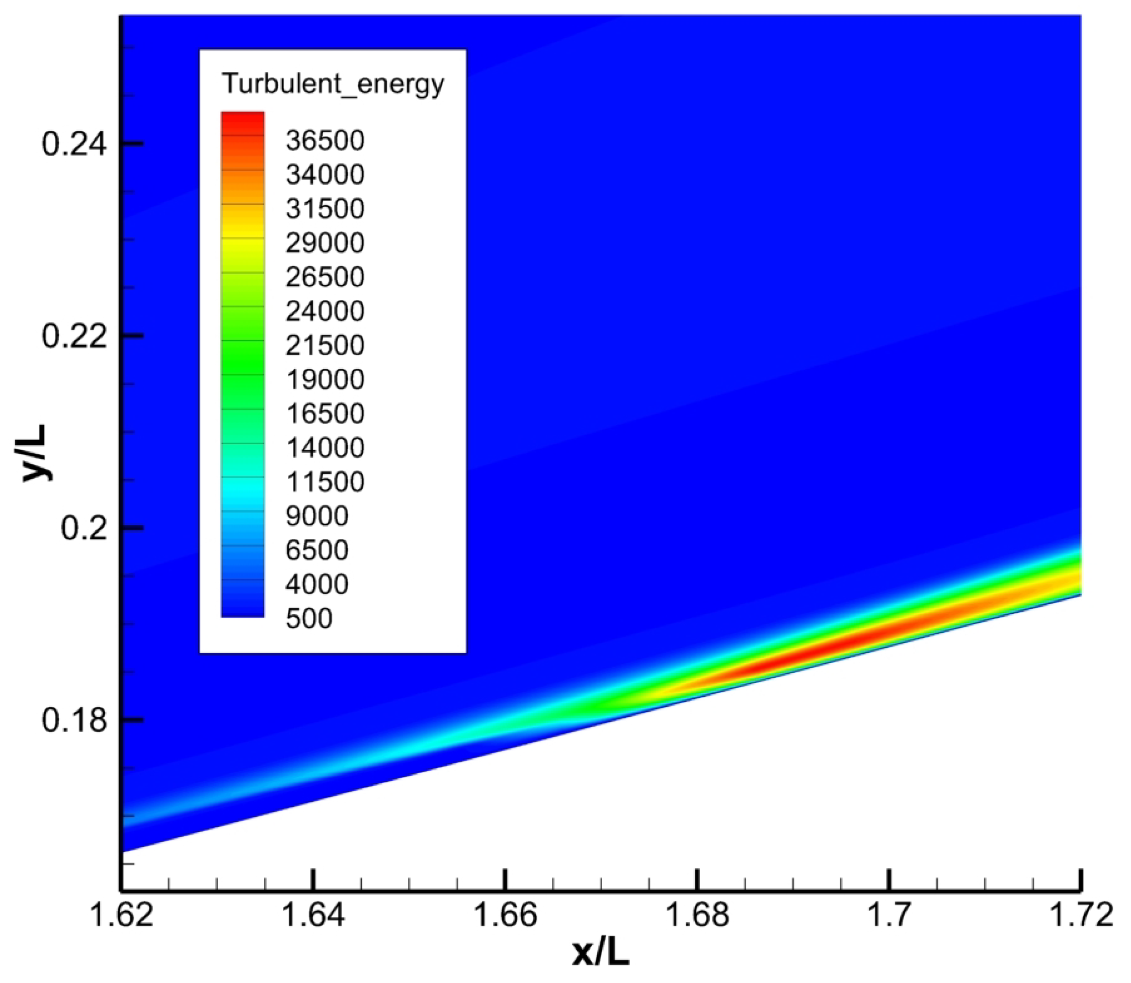
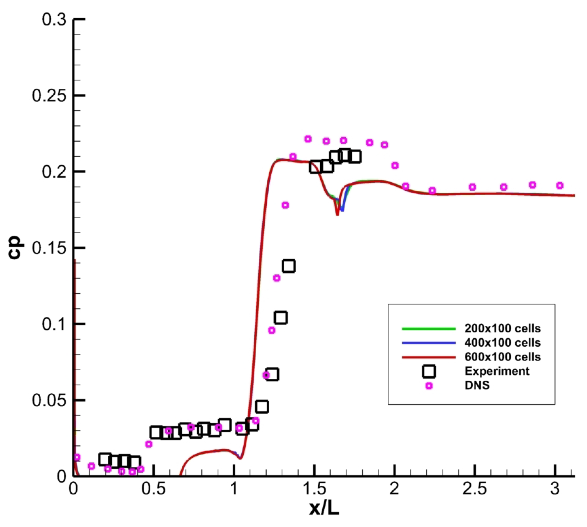
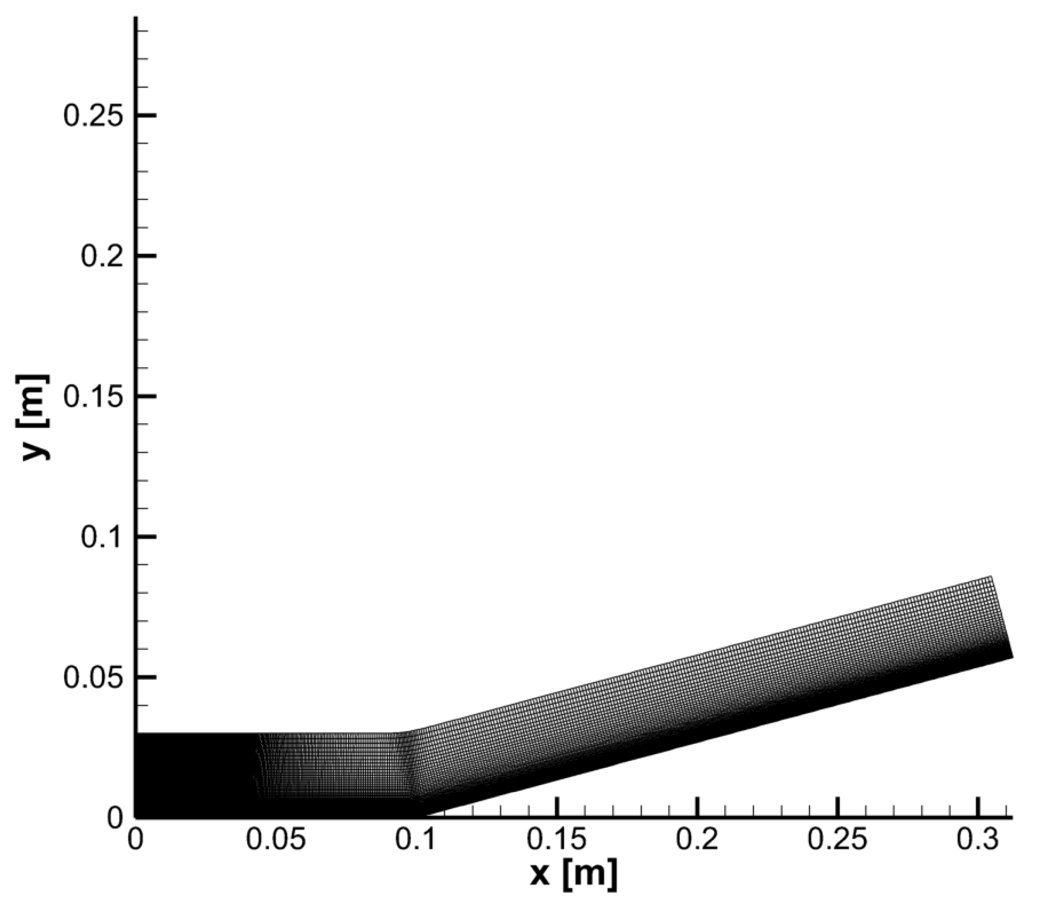
4. Numerical Solution of Hypersonic Flow over a Compressible Ramp

The hypersonic flow over a compressible ramp is characterized by the free-stream Mach number M = 7.7 and the Reynolds number R e = 8.6 · 10 5 . This setup corresponds to the same problem with total enthalpy h 0 = 1.7 MJ·kg 1 , as in the paper [7]. The relatively low total enthalpy allows a calorically perfect gas to be used as the fluid.
The simulation was performed in the computational domain shown in Figure 1. The lower boundary of the computational domain consists of a flat plate of length L = 100 mm, followed by a ramp of length 220 mm, with an angle of 15 degrees. The left boundary ( x = 0 ) of the computational domain and the upper boundary, which is equidistant by 30 mm from the lower boundary, are considered as inlet, while the right boundary is considered as outlet.
The computational domain was covered by a hyperbolically generated grid with 400 × 100 cells, with minimum grid spacing in the y-direction Δ y = 3.8 · 10 6 m, which corresponds to y + 0.9 .
The boundary conditions were prescribed in the following way:
  • Inlet: ρ = 0.032 kg · m 3 , u = 1726 m · s 1 , v = 0 m · s 1 , p = 1550 Pa , k = 111.7 m 2 · s 2 , and ω = 1.38 · 10 5 s 1 .
  • Outlet: zero-gradient extrapolation of all variables.
  • Solid wall (leading flat plate and compressible ramp): no-slip isothermal wall conditions, u w a l l = 0 m · s 1 , T w a l l = 293 K , k w a l l = 0 m 2 · s 2 , and ω w a l l = 1.668 · 10 9 s 1 .
The free-stream turbulent kinetic energy k was calculated using relation
k = 3 2 T u 2 | u | 2 ,
where the free-stream turbulence intensity T u is equal to half a percent, which is approximately the lower limit of the bypass transition model used in this work. Therefore, we are in the region between the natural transition and the bypass transition.
The free-stream value of the specific dissipation rate ω is based on the dimensional analysis
[ ω ] [ u ] [ L ] ω = C u L ,
where L is the characteristic size (in this case the length of the flat plate in front of the ramp), and C is constant of order O ( 1 ) . In our case, the value C = 7 is chosen because it allows us to correctly capture the transition onset.
Finally, the value of the specific dissipation rate ω w a l l is calculated using relation
ω w a l l = C ω 6 μ ρ β ( Δ y 1 / 2 ) 2 ,
which is based on the solution of the simplified Equation (9) in the near-wall region. Here, the constant C ω = 1.5 , and Δ y 1 / 2 is the distance between the center of the first cell and the wall.
Figure 2 shows the Mach number distribution. It shows a relatively weak shock wave generated by the leading edge of the flat plate and a separation bubble around the corner, with boundary layer separation located at x / L = 0.67 and reattachment at x / L = 1.17 . Both the separation and reattachment of the boundary layer generate stronger shock waves, which then interact at the so-called triple point located at x / L = 1.37 (Figure 3). The structure of the flow field is in good qualitative agreement with results obtained by the DNS method in [7].
Table 1 shows a comparison with the results obtained by the DNS method in [7]. There is a relatively large difference in the predicted location of the boundary layer separation compared to the DNS method. Since it is in the laminar part of the boundary layer, this difference is almost certainly due to the much more accurate numerical method and to the much finer grid used by the DNS method. On the other hand, the reattachment location is predicted reasonably well by the presented method. The difference in the predicted location of the triple point is due to above-mentioned shift in the separation location downstream. The shift of the triple point is caused by the change in the angle of the separation shock wave. Finally, the transition onset location is predicted, in good agreement with the DNS method.
Figure 4 shows the turbulent kinetic energy distribution. It shows a rather sharp transition onset located at x / L = 1.67 .
Figure 5 shows distributions of the pressure coefficient. A small pressure increase can be observed due to boundary layer separation and to a much higher increase downstream of the reattachment location. The first increase is predicted later compared to both the DNS method and the experiment. This is again due to the much higher accuracy of the DNS method. The second increase is predicted more accurately. A qualitatively different shape can be observed around the point x / L = 1.6 . This is due to the typical sharp bypass transition from the laminar to turbulent flow regime, which is notable even in the pressure distribution. The location of the pressure drop in the vicinity of x / L = 2 is predicted in good agreement with the DNS method, although the magnitude of the drop is smaller in the case of the presented method. Finally, the magnitude of the pressure coefficient in the turbulent part of the boundary layer is predicted in very good agreement with the DNS method.
A grid convergence study was also performed. The same problem was solved for three progressively refined meshes. The coarse mesh consists of 200 × 100 cells, the medium mesh of 400 × 100 cells, and fine mesh of 600 × 100 cells. Figure 5 shows all three results, which are almost indistinguishable. Therefore, the results can be considered to be grid-convergent.

5. Discussion and Conclusions

A numerical simulations of the hypersonic flow of viscous fluid over a compressible ramp with transition from laminar to turbulent flow regime has been performed.
The numerical solution was obtained by the common and much less demanding numerical method used on relatively coarse meshes (40–60 thousand cells) in comparison with the direct numerical simulation (627 million cells). This allows us to obtain solutions in a much shorter time, which is required for efficient analysis and industrial designs. This is clearly the biggest advantage of the presented method. On the other hand, the DNS method provides more accurate results that agree very well with the experiment, but at the cost of very long computation times (it can take months or even years, or it may be nearly impossible on current computers for cases with high Reynolds numbers). This makes the DNS method more suitable for research purposes or as a substitute for experiments.
Another advantage is the relative simplicity of the presented method, which can be used to solve more complex problems with complicated geometry, whereas the DNS method is generally only used for problems with simple geometry. Additionally, since many existing codes are based on the averaged Navier–Stokes equations and two-equation models of turbulence, it is easy to implement the presented method in existing solvers.
The lack of ability to model the natural transition is the biggest weakness of the presented method. The transition from a laminar to a turbulent flow regime is modeled by a very simple algebraic model of bypass transition, whereas the real transition process in the case of flow over a compressible ramp is probably caused by means of the natural one. This leads to a significant difference in the shape of the pressure coefficient distribution in the transition region.
Another weakness is the use of a numerical scheme with only second-order accuracy. There are visible differences (especially the location of the laminar boundary layer separation) in the solution due to the significantly lower accuracy of the presented method compared to the DNS. This could be resolved by using a higher-order reconstruction in space.
However, results obtained by the presented method are qualitatively correct and are reasonable accurate, at least for common industrial design applications. The computational time required to obtain a solution using the presented method is on the order of hours on commonly available computers. Therefore, it can be stated that the presented method has the potential to be used for design calculations of hypersonic vehicles.

Funding

This research received no external funding.

Data Availability Statement

Not applicable.

Acknowledgments

The work was supported by European Regional Development Fund-Project “Center for Advanced Applied Science” (No.CZ.02.1.01/0.0/0.0/16_019/0000778).

Conflicts of Interest

The authors declare no conflict of interest.

Abbreviations

The following abbreviations are used in this manuscript:
CFDComputational Fluid Dynamics
DNSDirect Numerical Simulation
EARSMExplicit Algebraic Reynolds Stresses Model
HLLHarten–Lax–van Leer
HLLCHarten–Lax–van Leer Contact
TVDTotal Variation Diminishing
WENOWeighted Essentially Non-Oscillatory

References

  1. Holman, J.; Fürst, J. Rotated-hybrid Riemann solver for all speed flows. J. Comput. Appl. Math. 2023, 427, 115129. [Google Scholar] [CrossRef]
  2. Qu, F.; Sun, D.; Liu, Q.; Bai, J. A Review of Riemann Solvers for Hypersonic Flows. Arch. Comput. Methods Eng. 2022, 29, 1771–1800. [Google Scholar] [CrossRef] [PubMed]
  3. Yang, X.; Zhang, Q.; Yuan, G.; Sheng, Z. On positivity preservation in nonlinear finite volume method for multi-term fractional subdiffusion equation on polygonal meshes. Nonlinear Dyn. 2018, 92, 595–612. [Google Scholar] [CrossRef]
  4. Yang, X.; Wu, L.; Zhang, H. A space-time spectral order sinc-collocation method for the fourth-order nonlocal heat model arising in viscoelasticity. Appl. Math. Comput. 2023, 457, 128192. [Google Scholar] [CrossRef]
  5. Zhang, R.; Liu, S.; Zhong, C.; Zhuo, C. Unified gas-kinetic scheme with simplified multi-scale numerical flux for thermodynamic non-equilibrium flow in all flow regimes. Commun. Nonlinear Sci. Numer. Simul. 2023, 119, 107079. [Google Scholar] [CrossRef]
  6. Wilcox, D.C. Turbulence Modeling for CFD; DCW Industries, Inc.: La Canada, CA, USA, 1994. [Google Scholar]
  7. Cao, S.; Hao, J.; Klioutchnikov, I.; Wen, C.-Y.; Olivier, H.; Heufer, K.A. Transition to turbulence in hypersonic flow over a compressible ramp due to intrinsic instability. J. Fluid Mech. 2022, 941, A8. [Google Scholar] [CrossRef]
  8. Bai, T.; Duan, Z.; Xiao, Z. Depth effects on the cavity induced transition at hypersonic speed by DNS. Int. J. Heat Fluid Flow 2022, 97, 109028. [Google Scholar] [CrossRef]
  9. Chen, X.; Dong, S.; Tu, G.; Yuan, X.; Chen, J. Boundary layer transition and linear modal instabilities of hypersonic flow over a lifting body. J. Fluid Mech. 2022, 938, A8. [Google Scholar] [CrossRef]
  10. Qi, H.; Li, X.; Yu, C.; Tong, F. Direct numerical simulation of hypersonic boundary layer transition over a lifting-body model HyTRV. Adv. Aerodyn. 2021, 3, 31. [Google Scholar] [CrossRef]
  11. Priebe, S.; Martín, M.P. Turbulence in a hypersonic compression ramp flow. Phys. Rev. Fluids 2021, 6, 034601. [Google Scholar] [CrossRef]
  12. Cao, S.; Hao, J.; Klioutchnikov, I.; Olivier, H.; Wen, C. Unsteady effects in a hypersonic compression ramp flow with laminar separation. J. Fluid Mech. 2021, 912, A3. [Google Scholar] [CrossRef]
  13. Cao, S.; Hao, J.; Guo, P.; Wen, C.; Klioutchnikov, I. Stability of hypersonic flow over a curved compression ramp. J. Fluid Mech. 2023, 957, A8. [Google Scholar] [CrossRef]
  14. Holman, J.; Fürst, J. Coupling the algebraic model of bypass transition with EARSM model of turbulence. Adv. Comput. Math. 2019, 45, 1977–1992. [Google Scholar] [CrossRef]
  15. Wallin, S.; Johansson, A. An explicit algebraic Reynolds stress model for incompressible and compressible turbulent flows. J. Fluid Mech. 2000, 403, 89–132. [Google Scholar] [CrossRef]
  16. Leveque, R.J. Finite-Volume Methods for Hyperbolic Problems; Cambridge University Press: Cambridge, UK, 2004. [Google Scholar]
  17. Friedrich, O. Weighted Essentially Non-Oscillatory Schemes for the Interpolation of Mean Values on Unstructured Grids. J. Comput. Phys. 1998, 144, 194–212. [Google Scholar] [CrossRef]
  18. Coirier, W. An Sdaptively-Refined, Cartesian, Cell-Based Scheme for the Euler and Navier-Stokes Equations. Ph.D. Thesis, University of Michigan, Ann Arbor, MI, USA, 1994. [Google Scholar]
  19. Gottlieb, S.; Shu, C.-W. Total Variation Diminishing Runge-Kutta Schemes. Math. Comput. 1996, 67, 73–85. [Google Scholar] [CrossRef]
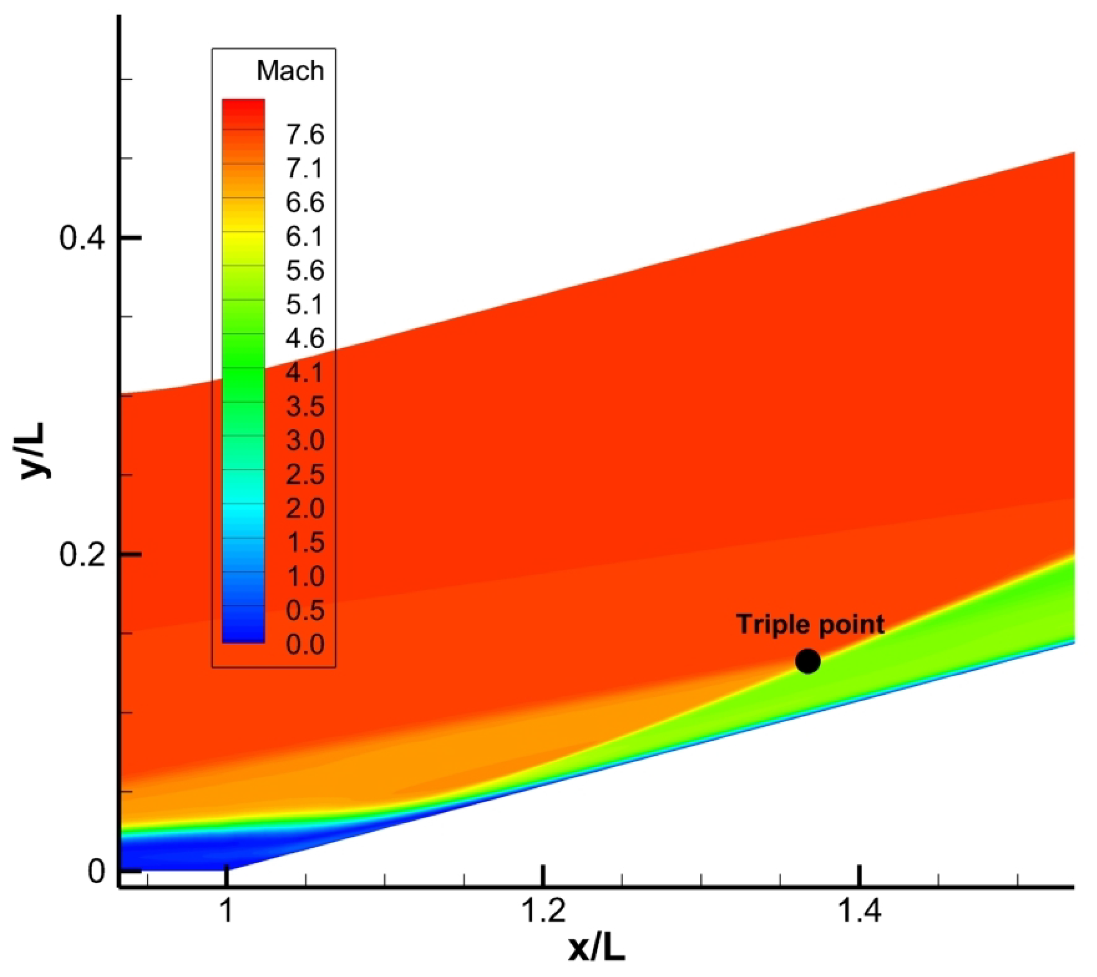
Figure 1. Computational domain and mesh.
Mathematics 11 03684 g001
Figure 2. Distribution of Mach number.
Mathematics 11 03684 g002
Figure 3. Distribution of Mach number; detail near the triple point.
Mathematics 11 03684 g003
Figure 4. Distribution of turbulent kinetic energy [ m 2 s 2 ]; detail near the transition onset.
Mathematics 11 03684 g004
Figure 5. Distributions of the pressure coefficient.
Mathematics 11 03684 g005
Table 1. Comparison of separation, reattachment, triple point, and transition locations.
MethodSeparationReattachmentTriple PointTransition
mod. EARSM0.671.171.371.67
DNS0.491.261.651.76
Disclaimer/Publisher’s Note: The statements, opinions and data contained in all publications are solely those of the individual author(s) and contributor(s) and not of MDPI and/or the editor(s). MDPI and/or the editor(s) disclaim responsibility for any injury to people or property resulting from any ideas, methods, instructions or products referred to in the content.

