
Dual Elite Groups-Guided Differential Evolution for Global Numerical Optimization


Abstract
:1. Introduction
2. Related Work
2.1. Differential Evolution
| Algorithm 1: The pseudocode of DE (DE/rand/1/bin) |
| Input: Population size PS, Scaling factor F, Crossover rate CR, Maximum fitness evaluations FESmax; |
|
| Output: f(x) and x |
2.2. Research on DE
2.2.1. Research on Mutation
2.2.2. Research on Parameter Adaptation
3. Proposed DEGGDE
3.1. DE/Current-to-Duelite/1
3.2. Difference between “DE/Current-to-Duelite/1” and Existing Similar Mutation Strategies
3.3. The Complete DEGGDE
| Algorithm 2: The pseudocode of DEGGDE |
| Input: Population size PS, Maximum fitness evaluations FESmax; |
|
| Output: f(gbest) and gbest |
4. Experiments
4.1. Experimental Setup
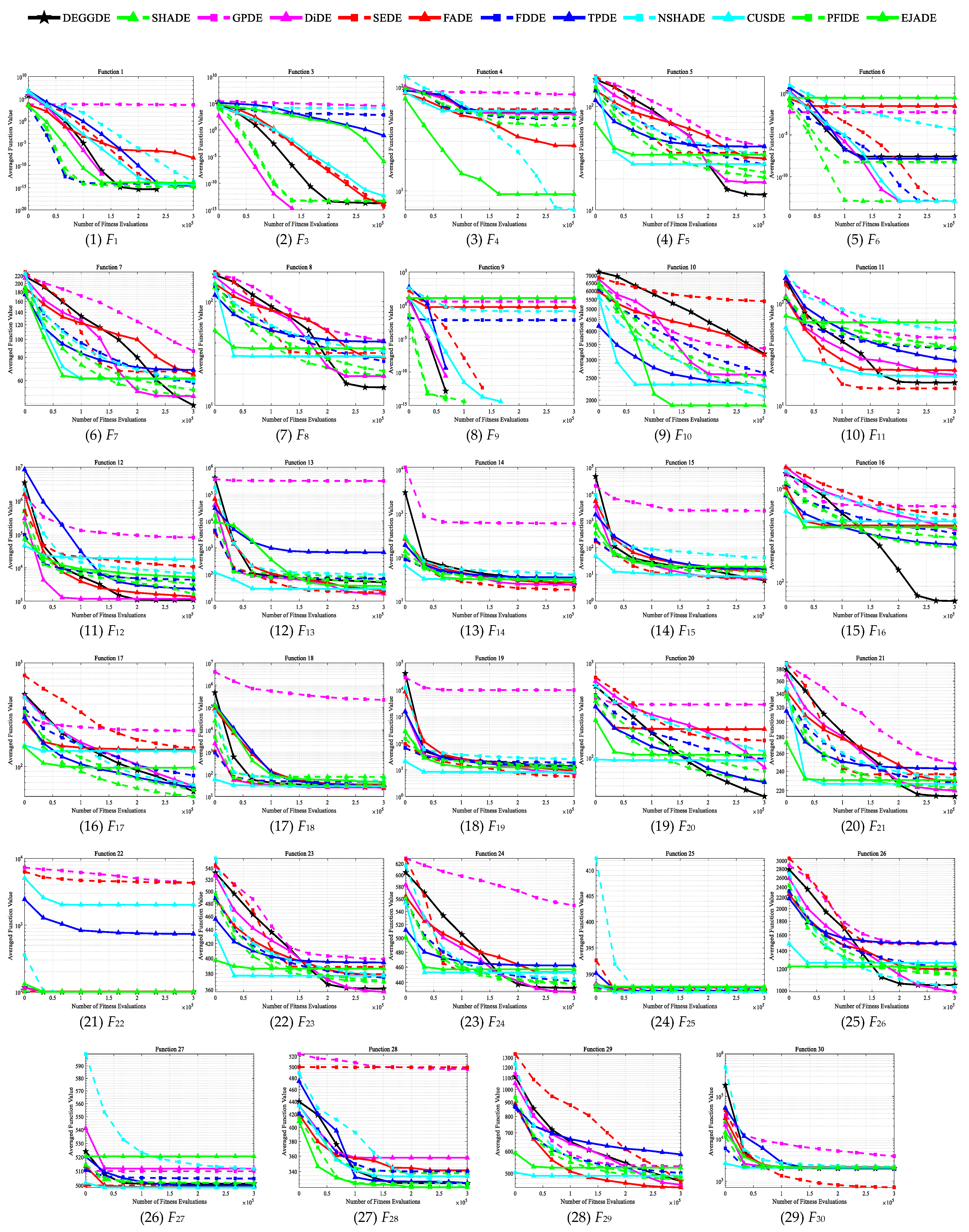
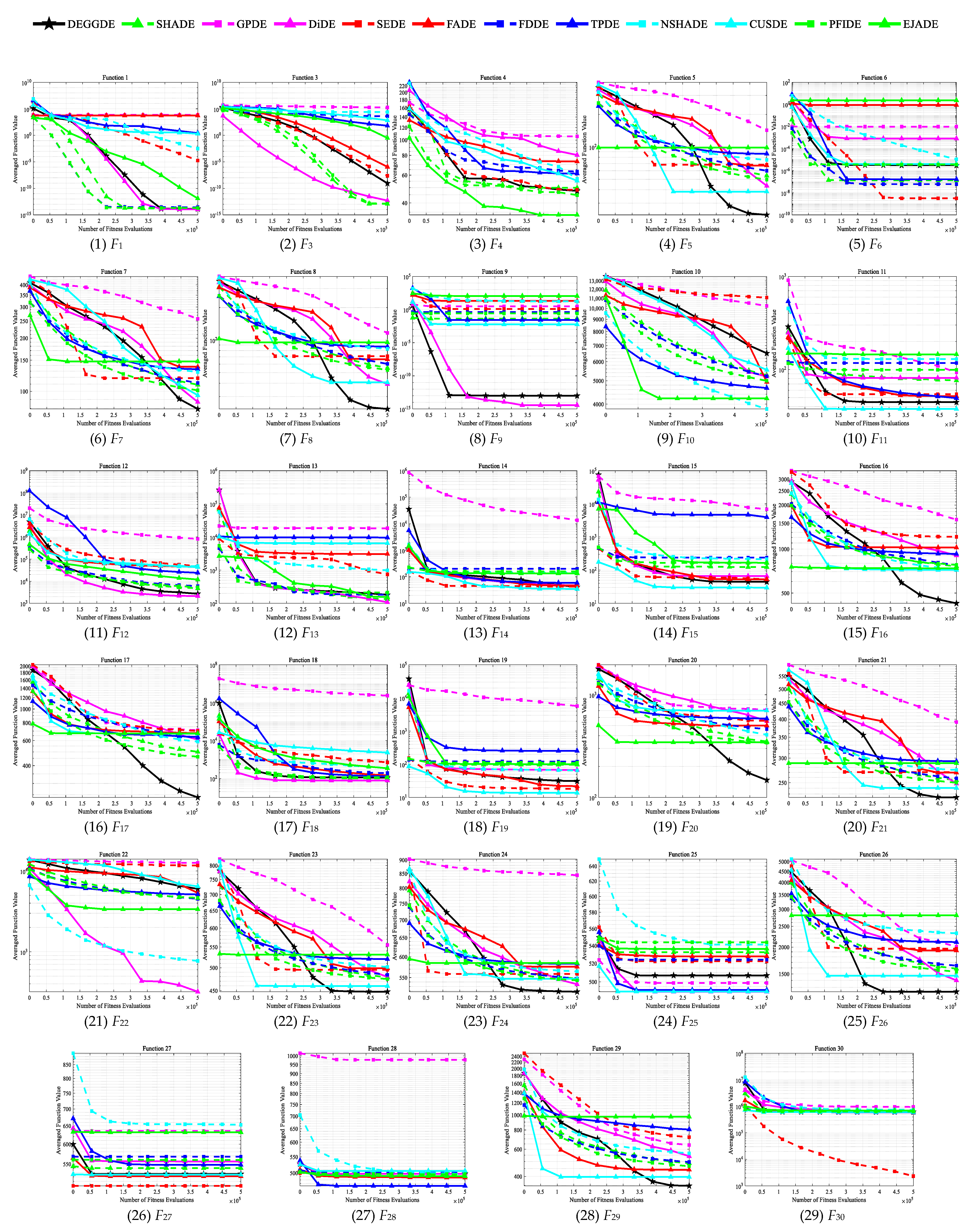
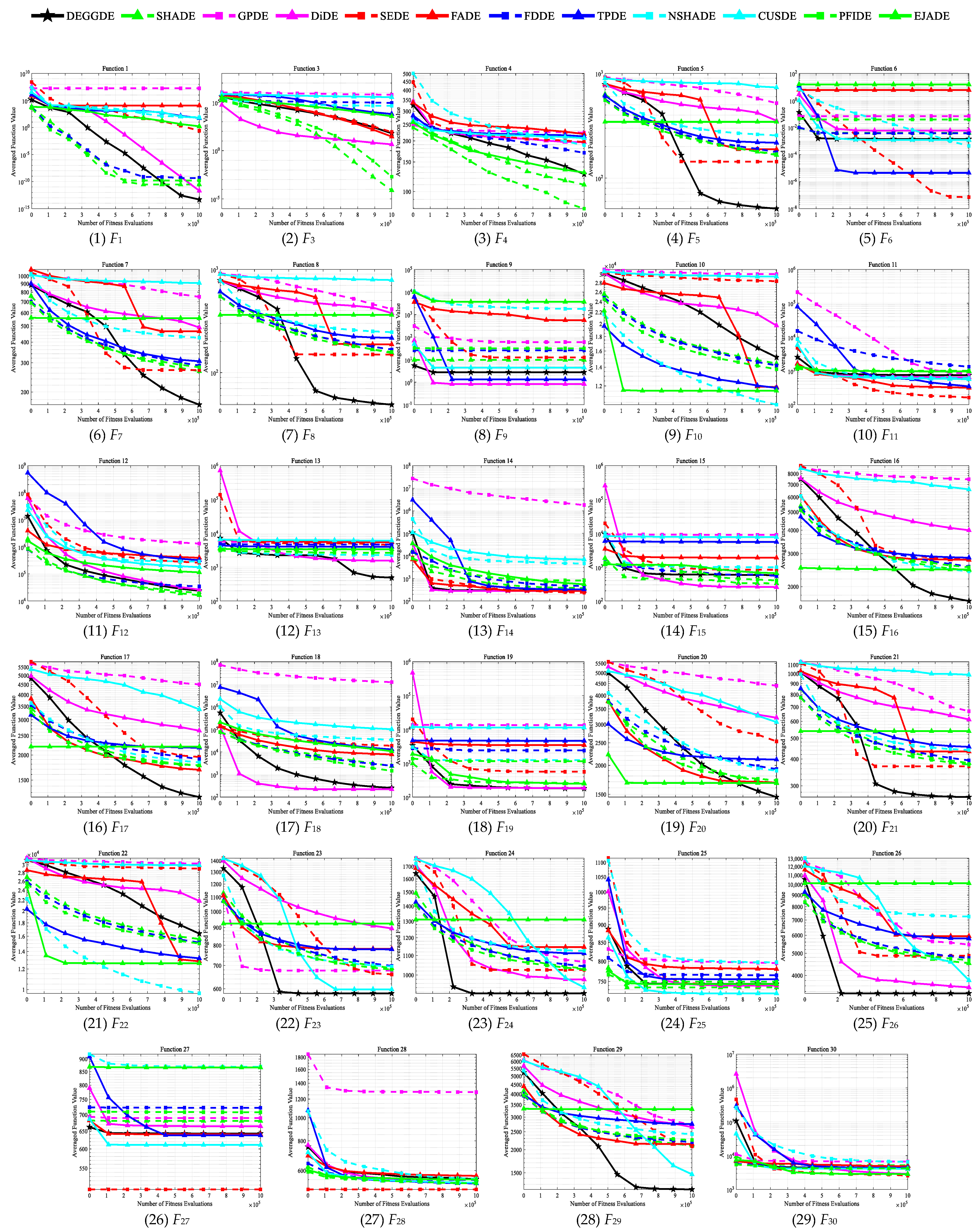
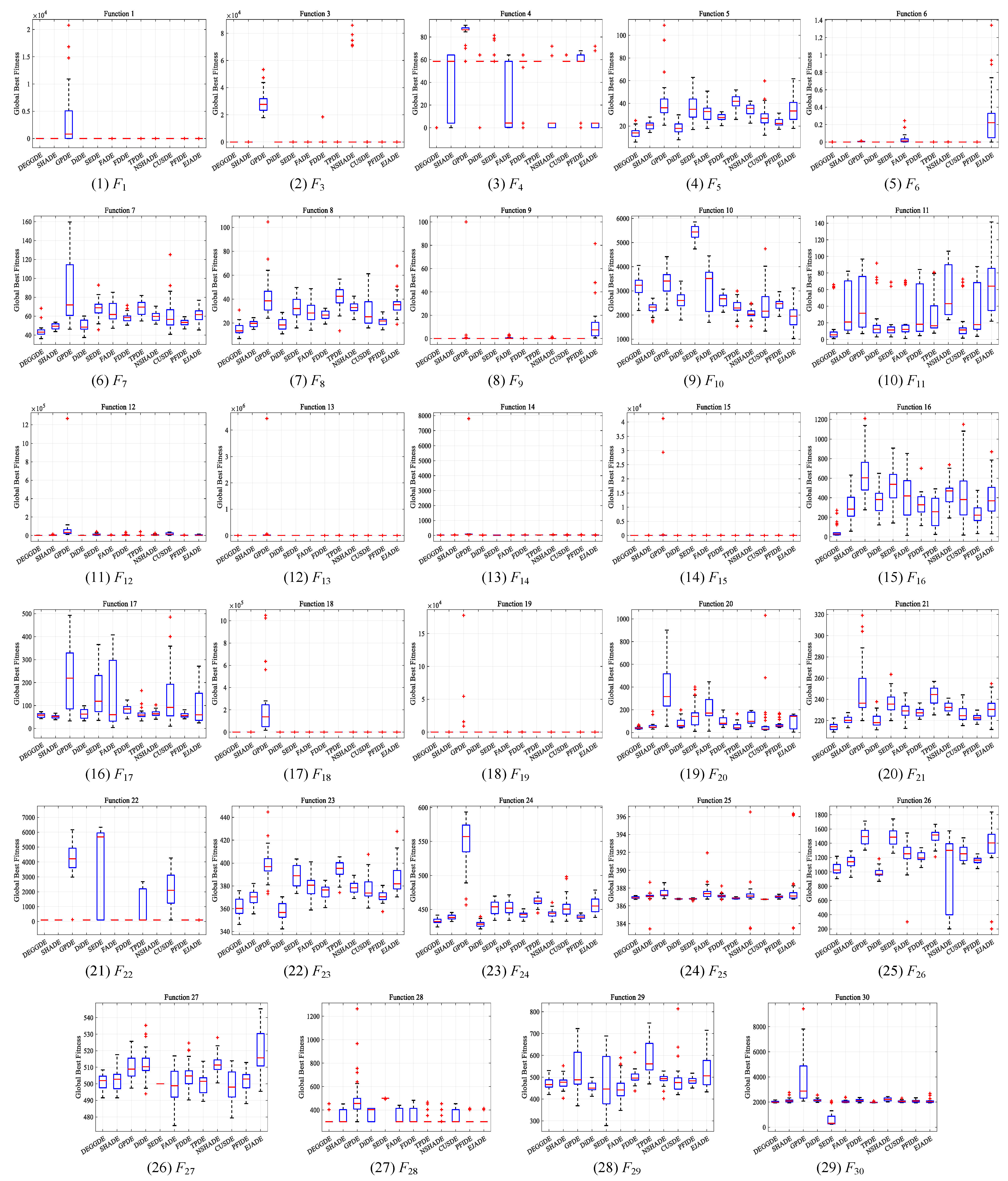
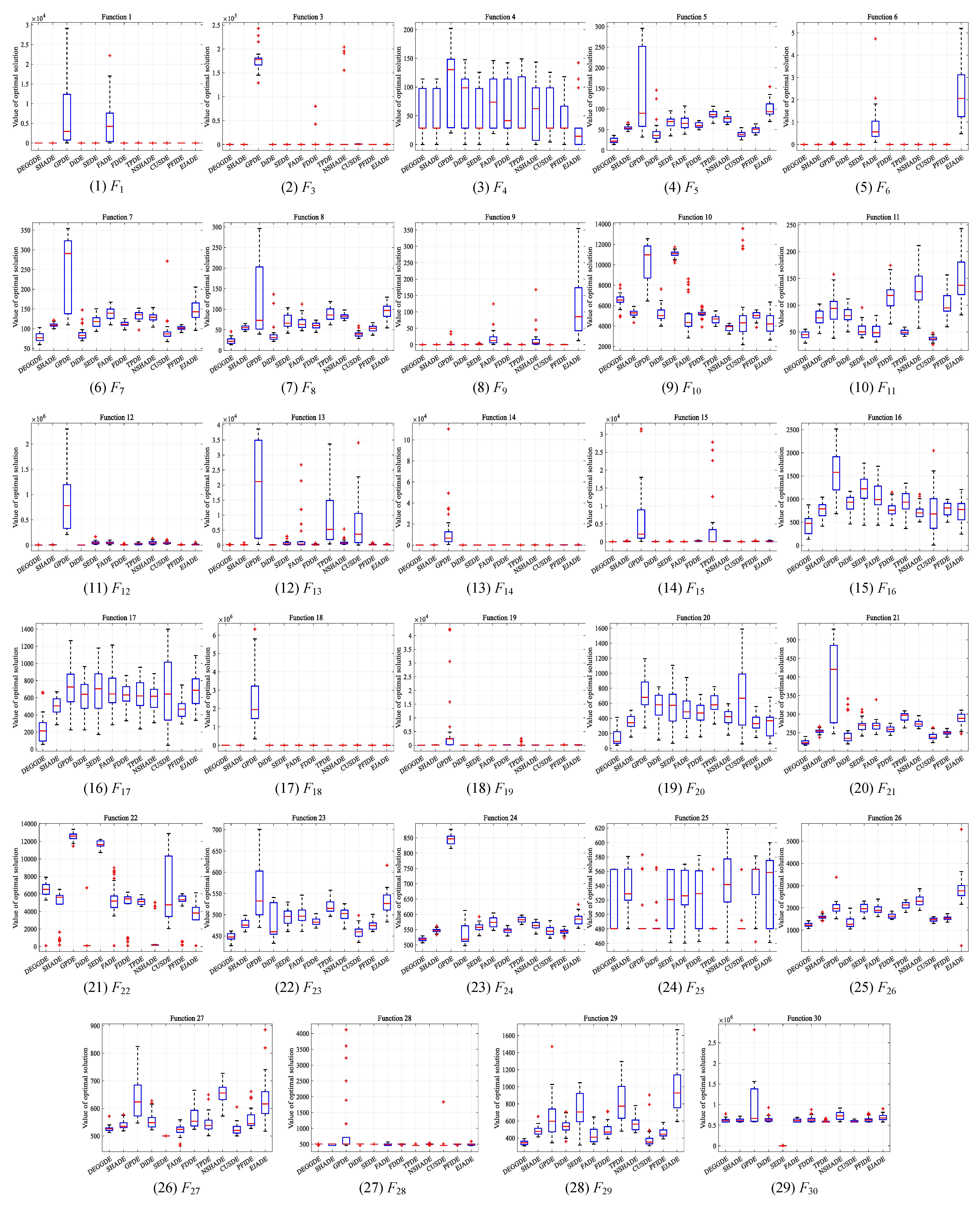
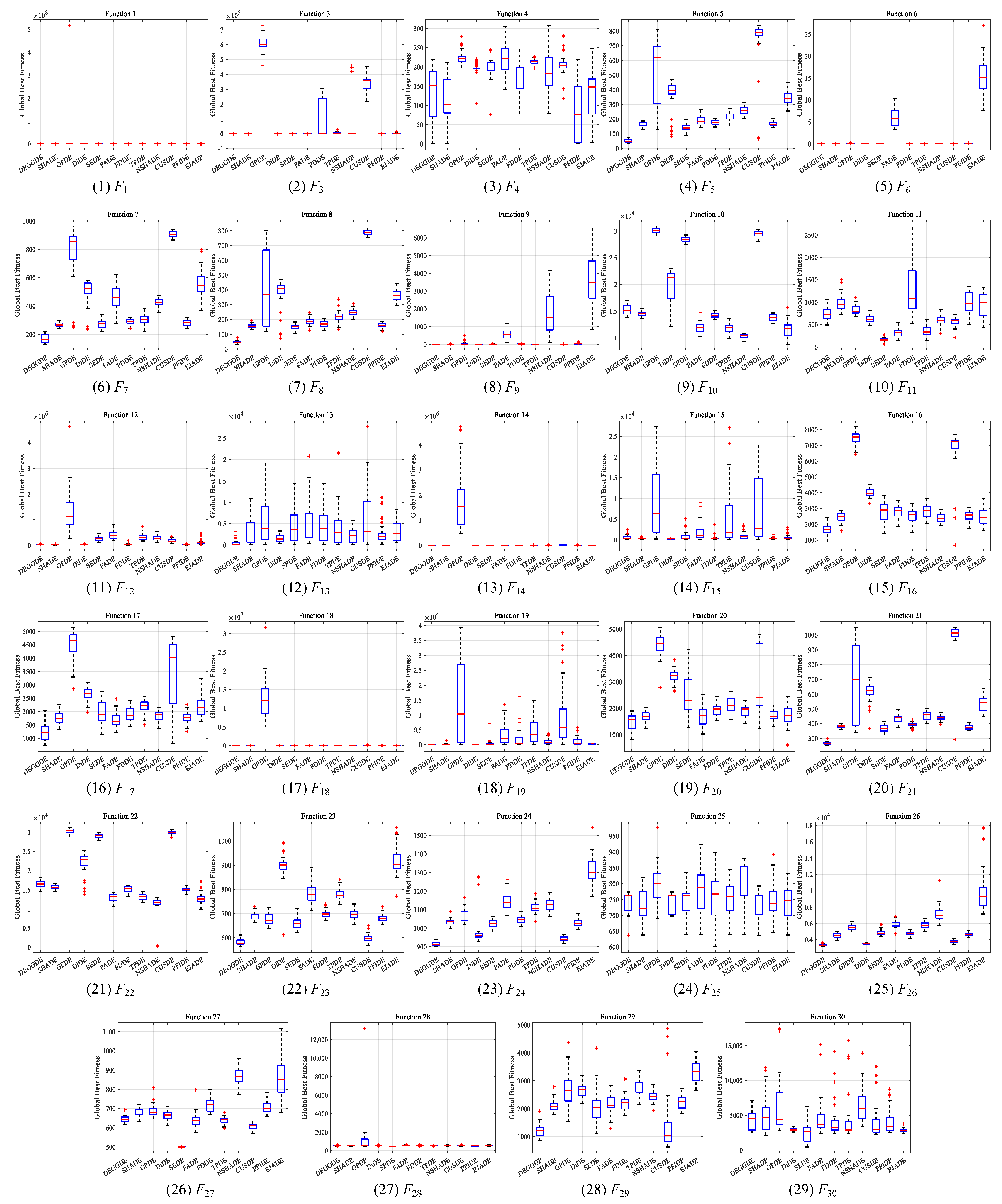
4.2. Comparisons between DEGGDE and State-of-the-Art DE Methods on the CEC’2017 Set
4.3. Deep Investigation on the Effectiveness of “DE/Current-to-Duelite/1”
5. Conclusions
Author Contributions
Funding
Data Availability Statement
Conflicts of Interest
References
- Storn, R.; Price, K. Differential evolution—A simple and efficient heuristic for global optimization over continuous spaces. J. Glob. Optim. 1997, 11, 341–359. [Google Scholar] [CrossRef]
- Zhang, J.; Chen, D.; Yang, Q.; Wang, Y.; Liu, D.; Jeon, S.-W.; Zhang, J. Proximity ranking-based multimodal differential evolution. Swarm Evol. Comput. 2023, 78, 101277. [Google Scholar] [CrossRef]
- Liu, D.; He, H.; Yang, Q.; Wang, Y.; Jeon, S.-W.; Zhang, J. Function value ranking aware differential evolution for global numerical optimization. Swarm Evol. Comput. 2023, 78, 101282. [Google Scholar] [CrossRef]
- Yang, Q.; Yan, J.-Q.; Gao, X.-D.; Xu, D.-D.; Lu, Z.-Y.; Zhang, J. Random neighbor elite guided differential evolution for global numerical optimization. Inf. Sci. 2022, 607, 1408–1438. [Google Scholar] [CrossRef]
- Zhou, S.; Xing, L.; Zheng, X.; Du, N.; Wang, L.; Zhang, Q. A self-adaptive differential evolution algorithm for scheduling a single batch-processing machine with arbitrary job sizes and release times. IEEE Trans. Cybern. 2021, 51, 1430–1442. [Google Scholar] [CrossRef]
- Xu, Y.; Pi, D.; Wu, Z.; Chen, J.; Zio, E. Hybrid discrete differential evolution and deep q-network for multimission selective maintenance. IEEE Trans. Reliab. 2022, 71, 1501–1512. [Google Scholar] [CrossRef]
- Liu, H.; Chen, Q.; Pan, N.; Sun, Y.; An, Y.; Pan, D. Uav stocktaking task-planning for industrial warehouses based on the improved hybrid differential evolution algorithm. IEEE Trans. Ind. Inform. 2022, 18, 582–591. [Google Scholar] [CrossRef]
- Brest, J.; Maučec, M.S.; Bošković, B. Single objective real-parameter optimization: Algorithm jso. In Proceedings of the IEEE Congress on Evolutionary Computation, Donostia, Spain, 5–8 June 2017; pp. 1311–1318. [Google Scholar]
- Awad, N.H.; Ali, M.Z.; Suganthan, P.N. Ensemble sinusoidal differential covariance matrix adaptation with euclidean neighborhood for solving cec2017 benchmark problems. In Proceedings of the IEEE Congress on Evolutionary Computation, Donostia, Spain, 5–8 June 2017; pp. 372–379. [Google Scholar]
- Tanabe, R.; Fukunaga, A.S. Improving the search performance of shade using linear population size reduction. In Proceedings of the IEEE Congress on Evolutionary Computation, Beijing, China, 6–11 July 2014; pp. 1658–1665. [Google Scholar]
- Liao, J.; Cai, Y.; Wang, T.; Tian, H.; Chen, Y. Cellular direction information based differential evolution for numerical optimization: An empirical study. Soft Comput. 2016, 20, 2801–2827. [Google Scholar] [CrossRef]
- Mohamed, A.W. An improved differential evolution algorithm with triangular mutation for global numerical optimization. Comput. Ind. Eng. 2015, 85, 359–375. [Google Scholar] [CrossRef]
- Opara, K.; Arabas, J. Comparison of mutation strategies in differential evolution—A probabilistic perspective. Swarm Evol. Comput. 2018, 39, 53–69. [Google Scholar] [CrossRef]
- Sun, G.; Cai, Y.; Wang, T.; Tian, H.; Wang, C.; Chen, Y. Differential evolution with individual-dependent topology adaptation. Inf. Sci. 2018, 450, 1–38. [Google Scholar] [CrossRef]
- Tian, M.; Gao, X.; Yan, X. Performance-driven adaptive differential evolution with neighborhood topology for numerical optimization. Knowl.-Based Syst. 2020, 188, 105008. [Google Scholar] [CrossRef]
- Ghosh, A.; Das, S.; Das, A.K.; Gao, L. Reusing the past difference vectors in differential evolution—A simple but significant improvement. IEEE Trans. Cybern. 2020, 50, 4821–4834. [Google Scholar] [CrossRef]
- Gong, W.; Cai, Z. Differential evolution with ranking-based mutation operators. IEEE Trans. Cybern. 2013, 43, 2066–2081. [Google Scholar] [CrossRef]
- Wang, C.; Gao, J. High-dimensional waveform inversion with cooperative coevolutionary differential evolution algorithm. IEEE Geosci. Remote Sens. Lett. 2012, 9, 297–301. [Google Scholar] [CrossRef]
- Wang, J.; Liao, J.; Zhou, Y.; Cai, Y. Differential evolution enhanced with multiobjective sorting-based mutation operators. IEEE Trans. Cybern. 2014, 44, 2792–2805. [Google Scholar] [CrossRef]
- Wang, K.; Gong, W.; Liao, Z.; Wang, L. Hybrid niching-based differential evolution with two archives for nonlinear equation system. IEEE Trans. Syst. Man Cybern. Syst. 2022, 52, 7469–7481. [Google Scholar] [CrossRef]
- Ji, W.X.; Yang, Q.; Gao, X.D. Gaussian sampling guided differential evolution based on elites for global optimization. IEEE Access 2023, 11, 80915–80944. [Google Scholar] [CrossRef]
- Hamza, N.M.; Essam, D.L.; Sarker, R.A. Constraint consensus mutation-based differential evolution for constrained optimization. IEEE Trans. Evol. Comput. 2016, 20, 447–459. [Google Scholar] [CrossRef]
- Xia, X.; Tong, L.; Zhang, Y.; Xu, X.; Yang, H.; Gui, L.; Li, Y.; Li, K. Nfdde: A novelty-hybrid-fitness driving differential evolution algorithm. Inf. Sci. 2021, 579, 33–54. [Google Scholar] [CrossRef]
- Zhao, X.; Xu, G.; Rui, L.; Liu, D.; Liu, H.; Yuan, J. A failure remember-driven self-adaptive differential evolution with top-bottom strategy. Swarm Evol. Comput. 2019, 45, 1–14. [Google Scholar] [CrossRef]
- Zou, L.; Pan, Z.; Gao, Z.; Gao, J. Improving the search accuracy of differential evolution by using the number of consecutive unsuccessful updates. Knowl.-Based Syst. 2022, 250, 109005. [Google Scholar] [CrossRef]
- Cai, Y.; Wu, D.; Zhou, Y.; Fu, S.; Tian, H.; Du, Y. Self-organizing neighborhood-based differential evolution for global optimization. Swarm Evol. Comput. 2020, 56, 100699. [Google Scholar] [CrossRef]
- Cheng, J.; Pan, Z.; Liang, H.; Gao, Z.; Gao, J. Differential evolution algorithm with fitness and diversity ranking-based mutation operator. Swarm Evol. Comput. 2021, 61, 100816. [Google Scholar] [CrossRef]
- Cai, Y.; Wang, J.; Yin, J. Learning-enhanced differential evolution for numerical optimization. Soft Comput. 2012, 16, 303–330. [Google Scholar] [CrossRef]
- Gao, Z.; Pan, Z.; Gao, J. Multimutation differential evolution algorithm and its application to seismic inversion. IEEE Trans. Geosci. Remote Sens. 2016, 54, 3626–3636. [Google Scholar] [CrossRef]
- Nadimi-Shahraki, M.H.; Taghian, S.; Mirjalili, S.; Faris, H. Mtde: An effective multi-trial vector-based differential evolution algorithm and its applications for engineering design problems. Appl. Soft Comput. 2020, 97, 106761. [Google Scholar] [CrossRef]
- Tan, Z.; Li, K.; Wang, Y. Differential evolution with adaptive mutation strategy based on fitness landscape analysis. Inf. Sci. 2021, 549, 142–163. [Google Scholar] [CrossRef]
- Xia, X.; Gui, L.; Zhang, Y.; Xu, X.; Yu, F.; Wu, H.; Wei, B.; He, G.; Li, Y.; Li, K. A fitness-based adaptive differential evolution algorithm. Inf. Sci. 2021, 549, 116–141. [Google Scholar] [CrossRef]
- Piotrowski, A.P. Adaptive memetic differential evolution with global and local neighborhood-based mutation operators. Inf. Sci. 2013, 241, 164–194. [Google Scholar] [CrossRef]
- Das, S.; Abraham, A.; Chakraborty, U.K.; Konar, A. Differential evolution using a neighborhood-based mutation operator. IEEE Trans. Evol. Comput. 2009, 13, 526–553. [Google Scholar] [CrossRef]
- Liu, X.f.; Zhan, Z.H.; Lin, Y.; Chen, W.N.; Gong, Y.J.; Gu, T.L.; Yuan, H.Q.; Zhang, J. Historical and heuristic-based adaptive differential evolution. IEEE Trans. Syst. Man Cybern. Syst. 2019, 49, 2623–2635. [Google Scholar] [CrossRef]
- Zhou, X.G.; Zhang, G.J. Differential evolution with underestimation-based multimutation strategy. IEEE Trans. Cybern. 2019, 49, 1353–1364. [Google Scholar] [CrossRef] [PubMed]
- Das, S.; Mandal, A.; Mukherjee, R. An adaptive differential evolution algorithm for global optimization in dynamic environments. IEEE Trans. Cybern. 2014, 44, 966–978. [Google Scholar] [CrossRef]
- Wang, Y.; Liu, Z.-Z.; Li, J.; Li, H.-X.; Yen, G.G. Utilizing cumulative population distribution information in differential evolution. Appl. Soft Comput. 2016, 48, 329–346. [Google Scholar] [CrossRef]
- Abbass, H.A. The self-adaptive pareto differential evolution algorithm. In Proceedings of the Congress on Evolutionary Computation, Honolulu, HI, USA, 12–17 May 2002; Volume 1, pp. 831–836. [Google Scholar]
- Das, S.; Konar, A.; Chakraborty, U. Two improved differential evolution schemes for faster global search. In Proceedings of the Annual Conference on Genetic and Evolutionary Computation, Washington, DC, USA, 25–29 June 2005; pp. 991–998. [Google Scholar]
- Qin, A.K.; Huang, V.L.; Suganthan, P.N. Differential evolution algorithm with strategy adaptation for global numerical optimization. IEEE Trans. Evol. Comput. 2009, 13, 398–417. [Google Scholar] [CrossRef]
- Draa, A.; Bouzoubia, S.; Boukhalfa, I. A sinusoidal differential evolution algorithm for numerical optimisation. Appl. Soft Comput. 2015, 27, 99–126. [Google Scholar] [CrossRef]
- Tang, L.; Dong, Y.; Liu, J. Differential evolution with an individual-dependent mechanism. IEEE Trans. Evol. Comput. 2015, 19, 560–574. [Google Scholar] [CrossRef]
- Zhou, Y.Z.; Yi, W.C.; Gao, L.; Li, X.Y. Adaptive differential evolution with sorting crossover rate for continuous optimization problems. IEEE Trans. Cybern. 2017, 47, 2742–2753. [Google Scholar] [CrossRef]
- Tanabe, R.; Fukunaga, A. Success-history based parameter adaptation for differential evolution. In Proceedings of the IEEE Congress on Evolutionary Computation, Cancun, Mexico, 20–23 June 2013; pp. 71–78. [Google Scholar]
- Zhang, J.; Sanderson, A.C. Jade: Adaptive differential evolution with optional external archive. IEEE Trans. Evol. Comput. 2009, 13, 945–958. [Google Scholar] [CrossRef]
- Cheng, S.; Liu, B.; Shi, Y.; Jin, Y.; Li, B. Evolutionary computation and big data: Key challenges and future directions. In Proceedings of the Data Mining and Big Data, Bali, Indonesia, 25–30 June 2016; pp. 3–14. [Google Scholar]
- Yang, Q.; Song, G.W.; Chen, W.N.; Jia, Y.H.; Gao, X.D.; Lu, Z.Y.; Jeon, S.W.; Zhang, J. Random contrastive interaction for particle swarm optimization in high-dimensional environment. IEEE Trans. Evol. Comput. 2023, 1. [Google Scholar] [CrossRef]
- Yang, Q.; Chen, W.N.; Gu, T.; Jin, H.; Mao, W.; Zhang, J. An adaptive stochastic dominant learning swarm optimizer for high-dimensional optimization. IEEE Trans. Cybern. 2022, 52, 1960–1976. [Google Scholar] [CrossRef]
- Bhattacharya, M.; Islam, R.; Abawajy, J. Evolutionary optimization: A big data perspective. J. Netw. Comput. Appl. 2016, 59, 416–426. [Google Scholar] [CrossRef]
- Yang, Q.; Song, G.-W.; Gao, X.-D.; Lu, Z.-Y.; Jeon, S.-W.; Zhang, J. A random elite ensemble learning swarm optimizer for high-dimensional optimization. Complex Intell. Syst. 2023, 1–34. [Google Scholar] [CrossRef]
- Price, K.V. An introduction to differential evolution. In New Ideas in Optimization; McGraw-Hill Inc.: New York, NY, USA, 1999. [Google Scholar]
- Ghosh, A.; Das, S.; Das, A.K.; Senkerik, R.; Viktorin, A.; Zelinka, I.; Masegosa, A.D. Using spatial neighborhoods for parameter adaptation: An improved success history based differential evolution. Swarm Evol. Comput. 2022, 71, 101057. [Google Scholar] [CrossRef]
- Yi, W.; Chen, Y.; Pei, Z.; Lu, J. Adaptive differential evolution with ensembling operators for continuous optimization problems. Swarm Evol. Comput. 2022, 69, 100994. [Google Scholar] [CrossRef]
- Awad, N.; Ali, M.; Liang, J.; Qu, B.; Suganthan, P. Problem definitions and evaluation criteria for the cec 2017 special session and competition on single objective bound constrained real-parameter numerical optimization. In Technical Report; Nanyang Technological University Singapore: Singapore, 2016; pp. 1–34. [Google Scholar]
- Storn, R.; Price, K. Minimizing the real functions of the icec’96 contest by differential evolution. In Proceedings of the IEEE International Conference on Evolutionary Computation, Nayoya, Japan, 20–22 May 1996; pp. 842–844. [Google Scholar]
- Price, K.V.; Storn, R.; Lampinen, J. Differential Evolution: A Practical Approach to Global Optimization; Springer Science & Business Media: Berlin, Germany, 2005. [Google Scholar]
- Baatar, N.; Zhang, D.; Koh, C.S. An improved differential evolution algorithm adopting λ -best mutation strategy for global optimization of electromagnetic devices. IEEE Trans. Magn. 2013, 49, 2097–2100. [Google Scholar] [CrossRef]
- Chen, S.; He, Q.; Zheng, C.; Sun, L.; Wang, X.; Ma, L.; Cai, Y. Differential evolution based simulated annealing method for vaccination optimization problem. IEEE Trans. Netw. Sci. Eng. 2022, 9, 4403–4415. [Google Scholar] [CrossRef]
- Das, S.; Suganthan, P.N. Differential evolution: A survey of the state-of-the-art. IEEE Trans. Evol. Comput. 2011, 15, 4–31. [Google Scholar] [CrossRef]
- Deng, W.; Xu, J.; Gao, X.Z.; Zhao, H. An enhanced msiqde algorithm with novel multiple strategies for global optimization problems. IEEE Trans. Syst. Man Cybern. Syst. 2022, 52, 1578–1587. [Google Scholar] [CrossRef]
- Eiben, A.E.; Hinterding, R.; Michalewicz, Z. Parameter control in evolutionary algorithms. IEEE Trans. Evol. Comput. 1999, 3, 124–141. [Google Scholar] [CrossRef]
- Fan, Q.; Yan, X. Self-adaptive differential evolution algorithm with zoning evolution of control parameters and adaptive mutation strategies. IEEE Trans. Cybern. 2016, 46, 219–232. [Google Scholar] [CrossRef] [PubMed]
- Li, H.; Gong, M.; Wang, C.; Miao, Q. Pareto self-paced learning based on differential evolution. IEEE Trans. Cybern. 2021, 51, 4187–4200. [Google Scholar] [CrossRef]
- Yang, Q.; Chen, W.N.; Deng, J.D.; Li, Y.; Gu, T.; Zhang, J. A level-based learning swarm optimizer for large-scale optimization. IEEE Trans. Evol. Comput. 2018, 22, 578–594. [Google Scholar] [CrossRef]
- Yang, Q.; Zhu, Y.; Gao, X.; Xu, D.; Lu, Z. Elite directed particle swarm optimization with historical information for high-dimensional problems. Mathematics 2022, 10, 1384. [Google Scholar] [CrossRef]
- Yang, Q.; Zhang, K.-X.; Gao, X.-D.; Xu, D.-D.; Lu, Z.-Y.; Jeon, S.-W.; Zhang, J. A dimension group-based comprehensive elite learning swarm optimizer for large-scale optimization. Mathematics 2022, 10, 1072. [Google Scholar] [CrossRef]
- Li, Y.; Wang, S.; Yang, B. An improved differential evolution algorithm with dual mutation strategies collaboration. Expert Syst. Appl. 2020, 153, 113451. [Google Scholar] [CrossRef]
- Deng, L.; Li, C.; Han, R.; Zhang, L.; Qiao, L. Tpde: A tri-population differential evolution based on zonal-constraint stepped division mechanism and multiple adaptive guided mutation strategies. Inf. Sci. 2021, 575, 22–40. [Google Scholar] [CrossRef]
- Cao, Z.; Wang, Z.; Fu, Y.; Jia, H.; Tian, F. An adaptive differential evolution framework based on population feature information. Inf. Sci. 2022, 608, 1416–1440. [Google Scholar] [CrossRef]
- Yang, Q.; Chen, W.N.; Li, Y.; Chen, C.L.P.; Xu, X.M.; Zhang, J. Multimodal estimation of distribution algorithms. IEEE Trans. Cybern. 2017, 47, 636–650. [Google Scholar] [CrossRef]
- Yang, Q.; Li, Y.; Gao, X.; Ma, Y.-Y.; Lu, Z.-Y.; Jeon, S.-W.; Zhang, J. An adaptive covariance scaling estimation of distribution algorithm. Mathematics 2021, 9, 3207. [Google Scholar] [CrossRef]
- Sun, J.; Gao, S.; Dai, H.; Cheng, J.; Zhou, M.; Wang, J. Bi-objective elite differential evolution algorithm for multivalued logic networks. IEEE Trans. Cybern. 2020, 50, 233–246. [Google Scholar] [CrossRef]
- Zhang, G.; Ma, X.; Wang, L.; Xing, K. Elite archive-assisted adaptive memetic algorithm for a realistic hybrid differentiation flowshop scheduling problem. IEEE Trans. Evol. Comput. 2022, 26, 100–114. [Google Scholar] [CrossRef]
- Yang, Q.; Hua, L.K.; Gao, X.; Xu, D.; Lu, Z.; Jeon, S.-W.; Zhang, J. Stochastic cognitive dominance leading particle swarm optimization for multimodal problems. Mathematics 2022, 10, 761. [Google Scholar] [CrossRef]
- Yang, Q.; Bian, Y.-W.; Gao, X.; Xu, D.; Lu, Z.; Jeon, S.-W.; Zhang, J. Stochastic triad topology based particle swarm optimization for global numerical optimization. Mathematics 2022, 10, 1032. [Google Scholar] [CrossRef]
- Yang, Q.; Guo, X.; Gao, X.; Xu, D.; Lu, Z. Differential elite learning particle swarm optimization for global numerical optimization. Mathematics 2022, 10, 1261. [Google Scholar] [CrossRef]
- Yang, Q.; Jing, Y.; Gao, X.; Xu, D.; Lu, Z.; Jeon, S.-W.; Zhang, J. Predominant cognitive learning particle swarm optimization for global numerical optimization. Mathematics 2022, 10, 1620. [Google Scholar] [CrossRef]
- Sun, G.; Lan, Y.; Zhao, R. Differential evolution with gaussian mutation and dynamic parameter adjustment. Soft Comput. 2019, 23, 1615–1642. [Google Scholar] [CrossRef]
- Meng, Z.; Yang, C.; Li, X.; Chen, Y. Di-de: Depth information-based differential evolution with adaptive parameter control for numerical optimization. IEEE Access 2020, 8, 40809–40827. [Google Scholar] [CrossRef]
- Liang, J.; Qiao, K.; Yu, K.; Ge, S.; Qu, B.; Xu, R.; Li, K. Parameters estimation of solar photovoltaic models via a self-adaptive ensemble-based differential evolution. Sol. Energy 2020, 207, 336–346. [Google Scholar] [CrossRef]
- Wang, Y.; Gao, S.; Yu, Y.; Cai, Z.; Wang, Z. A gravitational search algorithm with hierarchy and distributed framework. Knowl.-Based Syst. 2021, 218, 106877. [Google Scholar] [CrossRef]
- Xiao, T.-L.; Yang, Q.; Gao, X.-D.; Ma, Y.-Y.; Lu, Z.-Y.; Jeon, S.-W.; Zhang, J. Variation encoded large-scale swarm optimizers for path planning of unmanned aerial vehicle. In Proceedings of the Genetic and Evolutionary Computation Conference, Lisbon, Portugal, 15–19 July 2023; pp. 102–110. [Google Scholar]
- Lu, Z.; Liang, S.; Yang, Q.; Du, B. Evolving block-based convolutional neural network for hyperspectral image classification. IEEE Trans. Geosci. Remote Sens. 2022, 60, 5525921. [Google Scholar] [CrossRef]
- Gao, X.; Cao, W.; Yang, Q.; Wang, H.; Wang, X.; Jin, G.; Zhang, J. Parameter optimization of control system design for uncertain wireless power transfer systems using modified genetic algorithm. CAAI Trans. Intell. Technol. 2022, 7, 582–593. [Google Scholar] [CrossRef]
- Wei, F.F.; Chen, W.N.; Yang, Q.; Deng, J.; Luo, X.N.; Jin, H.; Zhang, J. A classifier-assisted level-based learning swarm optimizer for expensive optimization. IEEE Trans. Evol. Comput. 2021, 25, 219–233. [Google Scholar] [CrossRef]
- Chen, W.N.; Tan, D.Z.; Yang, Q.; Gu, T.; Zhang, J. Ant colony optimization for the control of pollutant spreading on social networks. IEEE Trans. Cybern. 2020, 50, 4053–4065. [Google Scholar] [CrossRef]


| Problem Type | Index | Problem Name | Optimum |
|---|---|---|---|
| Unimodal Problems | 1 | Shifted and Rotated Bent Cigar Problem | 100 |
| 3 | Shifted and Rotated Zakharov Problem | 300 | |
| Simple Multimodal Problems | 4 | Shifted and Rotated Rosenbrock’s Problem | 400 |
| 5 | Shifted and Rotated Rastrigin’s Problem | 500 | |
| 6 | Shifted and Rotated Expanded Scaffer’s F6 Problem | 600 | |
| 7 | Shifted and Rotated Lunacek Bi_Rastrigin Problem | 700 | |
| 8 | Shifted and Rotated Non-Continuous Rastrigin’s Problem | 800 | |
| 9 | Shifted and Rotated Levy Problem | 900 | |
| 10 | Shifted and Rotated Schwefel’s Problem | 1000 | |
| Hybrid Problems | 11 | Hybrid Problem 1 (N = 3) | 1100 |
| 12 | Hybrid Problem 2 (N = 3) | 1200 | |
| 13 | Hybrid Problem 3 (N = 3) | 1300 | |
| 14 | Hybrid Problem 4 (N = 4) | 1400 | |
| 15 | Hybrid Problem 5 (N = 4) | 1500 | |
| 16 | Hybrid Problem 6 (N = 4) | 1600 | |
| 17 | Hybrid Problem 6 (N = 5) | 1700 | |
| 18 | Hybrid Problem 6 (N = 5) | 1800 | |
| 19 | Hybrid Problem 6 (N = 5) | 1900 | |
| 20 | Hybrid Problem 6 (N = 6) | 2000 | |
| Composition Problems | 21 | Composition Problem 1 (N = 3) | 2100 |
| 22 | Composition Problem 2 (N = 3) | 2200 | |
| 23 | Composition Problem 3 (N = 4) | 2300 | |
| 24 | Composition Problem 4 (N = 4) | 2400 | |
| 25 | Composition Problem 5 (N = 5) | 2500 | |
| 26 | Composition Problem 6 (N = 5) | 2600 | |
| 27 | Composition Problem 7 (N = 6) | 2700 | |
| 28 | Composition Problem 8 (N = 6) | 2800 | |
| 29 | Composition Problem 9 (N = 3) | 2900 | |
| 30 | Composition Problem 10 (N = 3) | 3000 | |
| Search Range: | |||
| D | Parameter | DEGGDE | SHADE (2013) | GPDE (2019) | DiDE (2020) | SEDE (2020) | FADE (2021) | FDDE (2021) | TPDE (2021) | NSHADE (2022) | CUSDE (2022) | PFIDE (2022) | EJADE (2022) |
|---|---|---|---|---|---|---|---|---|---|---|---|---|---|
| 30 | PS | 230 | 110 | 30 | 300 | 50 | Initialized as 3 × 25 Adaptively Adjusted | 150 | 100 | 180 | 100 | 140 | 100 |
| 50 | 300 | 170 | 40 | 500 | 50 | 150 | 100 | 180 | 100 | 140 | 100 | ||
| 100 | 410 | 170 | 40 | 1000 | 80 | 150 | 100 | 190 | 100 | 140 | 100 |
| F | Category | Quality | DEGGDE | SHADE | GPDE | DiDE | SEDE | FADE | FDDE | TPDE | NSHADE | CUSDE | PFIDE | EJADE |
|---|---|---|---|---|---|---|---|---|---|---|---|---|---|---|
| F1 | Unimodal Functions | Mean | 0.00 × 100 | 5.60 × 10⁻¹⁵ | 4.13 × 10³ | 0.00 × 100 | 0.00 × 100 | 5.22 × 10⁻⁹ | 8.05 × 10⁻¹⁵ | 2.84 × 10⁻¹⁵ | 2.58 × 10⁻¹⁴ | 4.26 × 10⁻¹⁵ | 1.42 × 10⁻¹⁵ | 1.47 × 10⁻¹⁴ |
| Std | 0.00 × 100 | 6.98 × 10⁻¹⁵ | 6.02 × 10³ | 0.00 × 100 | 0.00 × 100 | 2.86 × 10⁻⁸ | 7.16 × 10⁻¹⁵ | 5.78 × 10⁻¹⁵ | 1.55 × 10⁻¹⁴ | 6.62 × 10⁻¹⁵ | 4.34 × 10⁻¹⁵ | 5.88 × 10⁻¹⁵ | ||
| p-value | – | 1.28 × 10⁻⁴ + | 1.21 × 10⁻¹² + | NaN = | NaN = | 8.27 × 10⁻⁷ + | 1.43 × 10⁻⁶ + | 1.09 × 10⁻² + | 6.59 × 10⁻¹³ + | 1.31 × 10⁻³ + | 8.14 × 10−2 = | 1.92 × 10⁻¹² + | ||
| F3 | Mean | 1.71 × 10⁻¹⁴ | 5.70 × 10⁻¹⁴ | 2.94 × 10⁴ | 0.00 × 100 | 3.80 × 10⁻¹⁵ | 1.14 × 10⁻¹⁴ | 6.15 × 10² | 8.72 × 10⁻² | 1.27 × 10⁴ | 4.26 × 10⁻¹³ | 5.12 × 10⁻¹⁴ | 1.24 × 10⁻⁶ | |
| Std | 2.66 × 10⁻¹⁴ | 1.50 × 10⁻¹⁴ | 8.09 × 10³ | 0.00 × 100 | 1.45 × 10⁻¹⁴ | 2.32 × 10⁻¹⁴ | 3.37 × 10³ | 2.06 × 10⁻¹ | 2.90 × 10⁴ | 2.08 × 10⁻¹³ | 1.73 × 10⁻¹⁴ | 6.80 × 10⁻⁶ | ||
| p-value | – | 1.10 × 10⁻⁷ + | 1.01 × 10⁻¹¹ + | 1.31 × 10⁻³ − | 2.12 × 10⁻² − | 3.80 × 10−1 = | 4.07 × 10⁻⁴ + | 1.01 × 10⁻¹¹ + | 1.01 × 10⁻¹¹ + | 9.70 × 10⁻¹² + | 1.71 × 10⁻² + | 9.21 × 10⁻⁵ + | ||
| F1–3 | w/t/l | – | 2/0/0 | 2/0/0 | 0/1/1 | 0/1/1 | 1/1/0 | 2/0/0 | 2/0/0 | 2/0/0 | 2/0/0 | 1/1/0 | 2/0/0 | |
| F4 | Simple Multimodal Functions | Mean | 5.66 × 101 | 4.30 × 101 | 8.51 × 101 | 5.50 × 101 | 6.10 × 101 | 2.73 × 101 | 5.00 × 101 | 5.86 × 101 | 6.55 × 100 | 5.87 × 101 | 5.12 × 101 | 9.31 × 100 |
| Std | 1.07 × 101 | 2.76 × 101 | 6.60 × 100 | 1.50 × 101 | 6.35 × 100 | 2.88 × 101 | 2.22 × 101 | 3.61 × 10⁻¹⁴ | 1.68 × 101 | 1.01 × 100 | 2.28 × 101 | 2.09 × 101 | ||
| p-value | – | 6.09 × 10−1 = | 1.70 × 10⁻¹² + | 2.75 × 10⁻⁷ − | 1.64 × 10⁻⁵ + | 3.06 × 10⁻³ − | 1.11 × 10⁻⁵ − | 2.71 × 10⁻¹⁴ + | 1.39 × 10⁻⁸ − | 4.29 × 10⁻¹⁴ + | 1.39 × 10⁻⁶ − | 1.24 × 10⁻⁷ − | ||
| F5 | Mean | 1.41 × 101 | 2.07 × 101 | 4.13 × 101 | 1.85 × 101 | 3.57 × 101 | 3.16 × 101 | 2.76 × 101 | 4.11 × 101 | 3.45 × 101 | 2.78 × 101 | 2.31 × 101 | 3.42 × 101 | |
| Std | 4.17 × 100 | 3.61 × 100 | 1.95 × 101 | 5.75 × 100 | 1.21 × 101 | 7.89 × 100 | 2.87 × 100 | 6.58 × 100 | 5.09 × 100 | 9.08 × 100 | 3.43 × 100 | 1.01 × 101 | ||
| p-value | – | 2.78 × 10⁻⁷ + | 4.95 × 10⁻¹¹ + | 1.27 × 10⁻³ + | 1.85 × 10⁻¹⁰ + | 1.14 × 10⁻¹⁰ + | 6.68 × 10⁻¹¹ + | 3.01 × 10⁻¹¹ + | 3.68 × 10⁻¹¹ + | 2.42 × 10⁻⁹ + | 2.03 × 10⁻⁹ + | 7.34 × 10⁻¹¹ + | ||
| F6 | Mean | 2.51 × 10⁻⁸ | 1.14 × 10⁻¹³ | 5.31 × 10⁻³ | 1.14 × 10⁻¹³ | 1.14 × 10⁻¹³ | 2.92 × 10⁻² | 1.14 × 10⁻¹³ | 1.37 × 10⁻⁸ | 4.42 × 10⁻⁵ | 1.14 × 10⁻¹³ | 5.70 × 10⁻⁹ | 2.86 × 10⁻¹ | |
| Std | 1.02 × 10⁻⁷ | 5.14 × 10⁻²⁹ | 2.42 × 10⁻³ | 5.14 × 10⁻²⁹ | 5.14 × 10⁻²⁹ | 5.28 × 10⁻² | 0.00 × 100 | 4.18 × 10⁻⁸ | 6.74 × 10⁻⁵ | 0.00 × 100 | 2.55 × 10⁻⁸ | 3.18 × 10⁻¹ | ||
| p-value | – | 1.70 × 10−1 = | 5.22 × 10⁻¹² + | 1.70 × 10−1 = | 1.70 × 10−1 = | 5.22 × 10⁻¹² + | 4.46 × 10⁻¹² − | 4.46 × 10⁻⁸ − | 5.22 × 10⁻¹² + | 4.46 × 10⁻¹² − | 2.77 × 10⁻⁹ − | 5.22 × 10⁻¹² + | ||
| F7 | Mean | 4.41 × 101 | 4.94 × 101 | 8.66 × 101 | 4.95 × 101 | 6.72 × 101 | 6.46 × 101 | 5.85 × 101 | 6.85 × 101 | 5.97 × 101 | 6.13 × 101 | 5.33 × 101 | 6.18 × 101 | |
| Std | 6.14 × 100 | 2.86 × 100 | 3.80 × 101 | 6.23 × 100 | 1.00 × 101 | 1.01 × 101 | 4.73 × 100 | 8.05 × 100 | 5.19 × 100 | 1.71 × 101 | 3.14 × 100 | 7.45 × 100 | ||
| p-value | 1.00 × 100 = | 4.11 × 10⁻⁷ + | 2.87 × 10⁻¹⁰ + | 3.77 × 10⁻⁴ + | 3.82 × 10⁻¹⁰ + | 8.10 × 10⁻¹⁰ + | 2.03 × 10⁻⁹ + | 1.78 × 10⁻¹⁰ + | 1.29 × 10⁻⁹ + | 7.69 × 10⁻⁸ + | 1.01 × 10⁻⁸ + | 1.86 × 10⁻⁹ + | ||
| F8 | Mean | 1.49 × 101 | 1.95 × 101 | 4.21 × 101 | 1.91 × 101 | 3.19 × 101 | 2.92 × 101 | 2.67 × 101 | 4.12 × 101 | 3.30 × 101 | 2.97 × 101 | 2.14 × 101 | 3.55 × 101 | |
| Std | 5.17 × 100 | 2.79 × 100 | 1.67 × 101 | 5.00 × 100 | 8.59 × 100 | 8.01 × 100 | 3.43 × 100 | 9.31 × 100 | 4.25 × 100 | 1.27 × 101 | 3.54 × 100 | 9.40 × 100 | ||
| p-value | – | 9.18 × 10⁻⁵ + | 5.43 × 10⁻¹¹ + | 1.80 × 10⁻³ + | 1.16 × 10⁻⁹ + | 3.96 × 10⁻⁹ + | 1.06 × 10⁻⁹ + | 1.94 × 10⁻¹⁰ + | 7.33 × 10⁻¹¹ + | 5.05 × 10⁻⁸ + | 1.10 × 10⁻⁶ + | 1.19 × 10⁻¹⁰ + | ||
| F9 | Mean | 0.00 × 100 | 0.00 × 100 | 3.56 × 100 | 0.00 × 100 | 0.00 × 100 | 5.45 × 10⁻¹ | 5.97 × 10⁻³ | 0.00 × 100 | 1.31 × 10⁻¹ | 0.00 × 100 | 0.00 × 100 | 1.24 × 101 | |
| Std | 0.00 × 100 | 0.00 × 100 | 1.82 × 101 | 0.00 × 100 | 0.00 × 100 | 8.39 × 10⁻¹ | 2.27 × 10⁻² | 0.00 × 100 | 3.12 × 10⁻¹ | 0.00 × 100 | 0.00 × 100 | 1.68 × 101 | ||
| p-value | – | NaN = | 1.20 × 10⁻¹² + | NaN = | NaN = | 1.29 × 10⁻⁷ + | 1.61 × 10−1 = | NaN = | 4.31 × 10⁻¹¹ + | NaN = | NaN = | 1.21 × 10⁻¹² + | ||
| F10 | Mean | 3.19 × 10³ | 2.29 × 10³ | 3.37 × 10³ | 2.58 × 10³ | 5.41 × 10³ | 3.15 × 10³ | 2.63 × 10³ | 2.33 × 10³ | 2.08 × 10³ | 2.34 × 10³ | 2.44 × 10³ | 1.90 × 10³ | |
| Std | 4.03 × 10² | 2.35 × 10² | 5.67 × 10² | 3.86 × 10² | 2.89 × 10² | 8.19 × 10² | 2.66 × 10² | 3.22 × 10² | 2.13 × 10² | 7.55 × 10² | 2.10 × 10² | 5.11 × 10² | ||
| p-value | – | 7.38 × 10⁻¹⁰ − | 9.33 × 10−2 = | 8.84 × 10⁻⁷ − | 3.02 × 10⁻¹¹ + | 3.26 × 10−1 = | 3.26 × 10⁻⁷ − | 3.20 × 10⁻⁹ − | 8.99 × 10⁻¹¹ − | 6.05 × 10⁻⁷ − | 5.00 × 10⁻⁹ − | 3.82 × 10⁻¹⁰ − | ||
| F4–10 | w/t/l | – | 3/3/1 | 6/1/0 | 3/2/2 | 5/2/0 | 5/1/1 | 3/1/3 | 4/1/2 | 5/0/2 | 4/1/2 | 3/1/3 | 5/0/2 | |
| F11 | Hybrid Functions | Mean | 1.67 × 101 | 3.71 × 101 | 4.61 × 101 | 2.00 × 101 | 1.47 × 101 | 2.21 × 101 | 3.55 × 101 | 2.74 × 101 | 5.46 × 101 | 1.93 × 101 | 3.63 × 101 | 6.55 × 101 |
| Std | 2.40 × 101 | 2.91 × 101 | 3.25 × 101 | 2.33 × 101 | 1.46 × 101 | 2.36 × 101 | 2.94 × 101 | 2.06 × 101 | 2.94 × 101 | 2.25 × 101 | 2.91 × 101 | 3.18 × 101 | ||
| p-value | – | 3.81 × 10⁻⁶ + | 4.09 × 10⁻⁷ + | 1.23 × 10⁻³ + | 2.55 × 10⁻³ − | 4.96 × 10⁻⁴ + | 3.58 × 10⁻⁵ + | 5.58 × 10⁻⁵ + | 1.72 × 10⁻⁶ + | 5.31 × 10⁻³ + | 1.24 × 10⁻⁵ + | 8.29 × 10⁻⁸ + | ||
| F12 | Mean | 1.08 × 10³ | 3.14 × 10³ | 8.01 × 10⁴ | 1.17 × 10³ | 1.07 × 10⁴ | 1.37 × 10³ | 4.37 × 10³ | 2.35 × 10³ | 6.75 × 10³ | 1.76 × 10⁴ | 1.60 × 10³ | 5.17 × 10³ | |
| Std | 3.08 × 10² | 2.88 × 10³ | 2.26 × 10⁵ | 3.73 × 10² | 9.86 × 10³ | 1.55 × 10³ | 6.63 × 10³ | 7.38 × 10³ | 6.10 × 10³ | 1.11 × 10⁴ | 8.18 × 10² | 3.98 × 10³ | ||
| p-value | – | 6.53 × 10⁻⁸ + | 3.02 × 10⁻¹¹ + | 3.87 × 10−1 = | 3.08 × 10⁻⁸ + | 2.34 × 10−1 = | 5.27 × 10⁻⁵ + | 1.09 × 10−1 = | 4.20 × 10⁻¹⁰ + | 3.02 × 10⁻¹¹ + | 1.24 × 10⁻³ + | 7.12 × 10⁻⁹ + | ||
| F13 | Mean | 4.96 × 101 | 6.59 × 101 | 3.08 × 10⁵ | 1.88 × 101 | 2.13 × 101 | 2.45 × 101 | 6.73 × 101 | 6.69 × 10² | 9.96 × 101 | 2.82 × 101 | 5.32 × 101 | 3.65 × 101 | |
| Std | 4.22 × 101 | 3.83 × 101 | 1.12 × 10⁶ | 7.17 × 100 | 6.15 × 100 | 9.74 × 100 | 4.37 × 101 | 1.52 × 10³ | 4.32 × 101 | 6.03 × 100 | 4.53 × 101 | 2.16 × 101 | ||
| p-value | – | 3.15 × 10⁻² + | 3.34 × 10⁻¹¹ + | 9.83 × 10⁻⁸ − | 3.52 × 10⁻⁷ − | 4.08 × 10⁻⁵ − | 6.97 × 10⁻³ + | 1.22 × 10⁻² + | 1.39 × 10⁻⁶ + | 2.53 × 10⁻⁴ − | 5.89 × 10−1 = | 1.62 × 10−1 = | ||
| F14 | Mean | 2.32 × 101 | 3.00 × 101 | 5.91 × 10² | 2.38 × 101 | 1.81 × 101 | 2.68 × 101 | 3.27 × 101 | 3.47 × 101 | 4.02 × 101 | 3.17 × 101 | 2.81 × 101 | 3.09 × 101 | |
| Std | 4.20 × 100 | 4.53 × 100 | 1.96 × 10³ | 4.22 × 100 | 1.17 × 101 | 7.80 × 100 | 6.02 × 100 | 2.60 × 100 | 8.59 × 100 | 1.02 × 101 | 6.75 × 100 | 8.18 × 100 | ||
| p-value | – | 1.70 × 10⁻⁸ + | 3.02 × 10⁻¹¹ + | 9.33 × 10−2 = | 6.31 × 10−1 = | 1.00 × 10⁻³ + | 2.92 × 10⁻⁹ + | 5.49 × 10⁻¹¹ + | 6.07 × 10⁻¹¹ + | 3.26 × 10⁻⁷ + | 7.60 × 10⁻⁷ + | 4.80 × 10⁻⁷ + | ||
| F15 | Mean | 5.95 × 100 | 1.67 × 101 | 2.43 × 10³ | 7.11 × 100 | 6.69 × 100 | 1.29 × 101 | 1.67 × 101 | 1.58 × 101 | 4.18 × 101 | 8.16 × 100 | 1.27 × 101 | 1.90 × 101 | |
| Std | 2.29 × 100 | 1.43 × 101 | 9.07 × 10³ | 4.10 × 100 | 3.65 × 100 | 5.49 × 100 | 1.30 × 101 | 2.76 × 100 | 3.17 × 101 | 5.27 × 100 | 9.68 × 100 | 1.34 × 101 | ||
| p-value | – | 1.87 × 10⁻⁵ + | 3.02 × 10⁻¹¹ + | 5.01 × 10−1 = | 8.42 × 10−1 = | 3.20 × 10⁻⁹ + | 1.39 × 10⁻⁶ + | 3.34 × 10⁻¹¹ + | 1.29 × 10⁻⁹ + | 4.21 × 10⁻² + | 1.60 × 10⁻⁷ + | 5.46 × 10⁻⁹ + | ||
| F16 | Mean | 6.26 × 101 | 3.00 × 10² | 6.46 × 10² | 3.67 × 10² | 5.23 × 10² | 4.03 × 10² | 3.31 × 10² | 2.53 × 10² | 4.57 × 10² | 4.47 × 10² | 2.36 × 10² | 3.86 × 10² | |
| Std | 7.53 × 101 | 1.44 × 10² | 2.44 × 10² | 1.32 × 10² | 1.94 × 10² | 2.39 × 10² | 1.23 × 10² | 1.50 × 10² | 1.22 × 10² | 3.33 × 10² | 1.17 × 10² | 1.90 × 10² | ||
| p-value | – | 2.23 × 10⁻⁹ + | 3.02 × 10⁻¹¹ + | 2.87 × 10⁻¹⁰ + | 8.15 × 10⁻¹¹ + | 1.60 × 10⁻⁷ + | 8.10 × 10⁻¹⁰ + | 2.38 × 10⁻⁷ + | 4.08 × 10⁻¹¹ + | 7.09 × 10⁻⁸ + | 3.65 × 10⁻⁸ + | 5.07 × 10⁻¹⁰ + | ||
| F17 | Hybrid Functions | Mean | 5.77 × 101 | 5.15 × 101 | 2.23 × 10² | 6.46 × 101 | 1.51 × 10² | 1.46 × 10² | 8.20 × 101 | 6.27 × 101 | 6.67 × 101 | 1.41 × 10² | 5.96 × 101 | 9.73 × 101 |
| Std | 9.41 × 100 | 6.83 × 100 | 1.45 × 10² | 1.92 × 101 | 9.82 × 101 | 1.40 × 10² | 2.00 × 101 | 2.48 × 101 | 1.44 × 101 | 1.21 × 10² | 1.13 × 101 | 6.69 × 101 | ||
| p-value | – | 1.44 × 10⁻² − | 3.81 × 10⁻⁷ + | 2.90 × 10−1 = | 1.64 × 10⁻⁵ + | 3.95 × 10−1 = | 2.49 × 10⁻⁶ + | 7.84 × 10−1 = | 1.44 × 10⁻² + | 4.03 × 10⁻³ + | 5.89 × 10−1 = | 4.29 × 10−1 = | ||
| F18 | Mean | 2.55 × 101 | 7.57 × 101 | 2.19 × 10⁵ | 2.49 × 101 | 2.64 × 101 | 3.43 × 101 | 4.54 × 101 | 3.03 × 101 | 5.13 × 101 | 2.88 × 101 | 3.13 × 101 | 4.56 × 101 | |
| Std | 3.04 × 100 | 5.70 × 101 | 2.66 × 10⁵ | 3.67 × 100 | 5.28 × 100 | 1.07 × 101 | 2.74 × 101 | 2.52 × 100 | 2.19 × 101 | 9.32 × 100 | 9.61 × 100 | 3.16 × 101 | ||
| p-value | – | 3.65 × 10⁻⁸ + | 3.02 × 10⁻¹¹ + | 4.12 × 10−1 = | 9.05 × 10−2 = | 7.69 × 10⁻⁸ + | 7.22 × 10⁻⁶ + | 8.20 × 10⁻⁷ + | 1.78 × 10⁻¹⁰ + | 9.33 × 10−2 = | 6.97 × 10⁻³ + | 1.25 × 10⁻⁵ + | ||
| F19 | Mean | 1.09 × 101 | 1.59 × 101 | 9.63 × 10³ | 7.41 × 100 | 5.67 × 100 | 9.24 × 100 | 1.86 × 101 | 1.39 × 101 | 2.47 × 101 | 8.24 × 100 | 1.27 × 101 | 1.18 × 101 | |
| Std | 3.04 × 100 | 7.18 × 100 | 3.35 × 10⁴ | 2.73 × 100 | 2.12 × 100 | 3.86 × 100 | 1.34 × 101 | 1.85 × 100 | 5.40 × 100 | 2.29 × 100 | 3.86 × 100 | 5.70 × 100 | ||
| p-value | – | 2.50 × 10⁻³ + | 1.61 × 10⁻¹⁰ + | 4.35 × 10⁻⁵ − | 5.09 × 10⁻⁸ − | 3.18 × 10⁻³ − | 1.17 × 10⁻⁵ + | 7.20 × 10⁻⁵ + | 1.21 × 10⁻¹⁰ + | 2.39 × 10⁻⁴ − | 8.24 × 10−2 = | 9.23 × 10−1 = | ||
| F20 | Mean | 3.88 × 101 | 5.67 × 101 | 3.63 × 10² | 7.86 × 101 | 1.51 × 10² | 2.00 × 10² | 9.64 × 101 | 5.48 × 101 | 1.16 × 10² | 9.38 × 101 | 7.21 × 101 | 1.07 × 10² | |
| Std | 9.42 × 100 | 3.32 × 101 | 1.97 × 10² | 4.12 × 101 | 1.08 × 10² | 1.21 × 10² | 4.27 × 101 | 3.25 × 101 | 4.75 × 101 | 1.98 × 10² | 3.65 × 101 | 5.82 × 101 | ||
| p-value | – | 8.66 × 10⁻⁵ + | 3.69 × 10⁻¹¹ + | 6.53 × 10⁻⁸ + | 1.17 × 10⁻⁵ + | 1.61 × 10⁻⁶ + | 9.92 × 10⁻¹¹ + | 1.91 × 10−1 = | 6.70 × 10⁻¹¹ + | 9.93 × 10−2 = | 5.00 × 10⁻⁹ + | 2.62 × 10⁻³ + | ||
| F11–20 | w/t/l | – | 9/0/1 | 10/0/0 | 3/5/2 | 4/3/3 | 6/2/2 | 10/0/0 | 7/3/0 | 10/0/0 | 6/2/2 | 7/3/0 | 7/3/0 | |
| F21 | Composition Functions | Mean | 2.14 × 10² | 2.21 × 10² | 2.48 × 10² | 2.20 × 10² | 2.37 × 10² | 2.29 × 10² | 2.28 × 10² | 2.43 × 10² | 2.33 × 10² | 2.27 × 10² | 2.23 × 10² | 2.31 × 10² |
| Std | 3.50 × 100 | 3.42 × 100 | 2.69 × 101 | 6.32 × 100 | 1.02 × 101 | 7.36 × 100 | 4.17 × 100 | 8.38 × 100 | 4.55 × 100 | 7.43 × 100 | 3.31 × 100 | 9.75 × 100 | ||
| p-value | – | 5.53 × 10⁻⁸ + | 4.08 × 10⁻¹¹ + | 8.15 × 10⁻⁵ + | 5.49 × 10⁻¹¹ + | 9.76 × 10⁻¹⁰ + | 4.50 × 10⁻¹¹ + | 3.02 × 10⁻¹¹ + | 3.02 × 10⁻¹¹ + | 1.07 × 10⁻⁹ + | 1.41 × 10⁻⁹ + | 1.29 × 10⁻⁹ + | ||
| F22 | Mean | 1.00 × 10² | 1.00 × 10² | 4.29 × 10³ | 1.00 × 10² | 4.28 × 10³ | 1.01 × 10² | 1.00 × 10² | 7.38 × 10² | 1.00 × 10² | 2.02 × 10³ | 1.00 × 10² | 1.00 × 10² | |
| Std | 0.00 × 100 | 0.00 × 100 | 1.19 × 10³ | 0.00 × 100 | 2.58 × 10³ | 1.78 × 100 | 0.00 × 100 | 1.08 × 10³ | 2.23 × 10⁻¹³ | 1.32 × 10³ | 0.00 × 100 | 7.54 × 10⁻¹ | ||
| p-value | – | NaN = | 1.21 × 10⁻¹² + | NaN = | 1.70 × 10⁻⁸ + | 1.37 × 10⁻³ + | 1.69 × 10⁻¹⁴ − | 6.54 × 10⁻⁴ + | 1.79 × 10⁻⁷ + | 1.52 × 10⁻⁴ + | 1.69 × 10⁻¹⁴ − | 1.94 × 10⁻⁹ + | ||
| F23 | Mean | 3.61 × 10² | 3.70 × 10² | 3.99 × 10² | 3.58 × 10² | 3.89 × 10² | 3.80 × 10² | 3.75 × 10² | 3.94 × 10² | 3.79 × 10² | 3.77 × 10² | 3.71 × 10² | 3.87 × 10² | |
| Std | 7.76 × 100 | 6.12 × 100 | 1.42 × 101 | 7.48 × 100 | 9.36 × 100 | 1.04 × 101 | 5.81 × 100 | 7.26 × 100 | 5.09 × 100 | 1.06 × 101 | 5.20 × 100 | 1.39 × 101 | ||
| p-value | – | 7.20 × 10⁻⁵ + | 4.08 × 10⁻¹¹ + | 7.48 × 10−2 = | 4.50 × 10⁻¹¹ + | 2.60 × 10⁻⁸ + | 2.83 × 10⁻⁸ + | 3.34 × 10⁻¹¹ + | 2.37 × 10⁻¹⁰ + | 6.01 × 10⁻⁸ + | 1.17 × 10⁻⁵ + | 1.46 × 10⁻¹⁰ + | ||
| F24 | Mean | 4.33 × 10² | 4.38 × 10² | 5.50 × 10² | 4.28 × 10² | 4.53 × 10² | 4.53 × 10² | 4.42 × 10² | 4.62 × 10² | 4.45 × 10² | 4.53 × 10² | 4.39 × 10² | 4.57 × 10² | |
| Std | 4.06 × 100 | 3.62 × 100 | 3.53 × 101 | 4.21 × 100 | 9.65 × 100 | 9.26 × 100 | 4.56 × 100 | 6.85 × 100 | 5.69 × 100 | 1.55 × 101 | 3.05 × 100 | 1.22 × 101 | ||
| p-value | – | 8.29 × 10⁻⁶ + | 3.02 × 10⁻¹¹ + | 4.35 × 10⁻⁵ − | 1.61 × 10⁻¹⁰ + | 1.21 × 10⁻¹⁰ + | 2.39 × 10⁻⁸ + | 3.02 × 10⁻¹¹ + | 1.86 × 10⁻⁹ + | 1.17 × 10⁻⁹ + | 1.03 × 10⁻⁶ + | 6.70 × 10⁻¹¹ + | ||
| F25 | Mean | 3.87 × 10² | 3.87 × 10² | 3.87 × 10² | 3.87 × 10² | 3.87 × 10² | 3.88 × 10² | 3.87 × 10² | 3.87 × 10² | 3.87 × 10² | 3.87 × 10² | 3.87 × 10² | 3.88 × 10² | |
| Std | 1.09 × 10⁻¹ | 7.64 × 10⁻¹ | 5.24 × 10⁻¹ | 3.59 × 10⁻² | 5.88 × 10⁻² | 9.47 × 10⁻¹ | 2.70 × 10⁻¹ | 7.33 × 10⁻² | 2.02 × 100 | 1.94 × 10⁻² | 1.43 × 10⁻¹ | 3.22 × 100 | ||
| p-value | – | 9.79 × 10⁻⁵ + | 2.01 × 10⁻⁸ + | 3.80 × 10⁻⁷ − | 8.83 × 10⁻⁷ − | 2.32 × 10⁻⁶ + | 7.66 × 10⁻⁵ + | 1.03 × 10⁻² − | 5.87 × 10⁻⁴ + | 5.03 × 10⁻¹⁰ − | 2.05 × 10⁻³ + | 2.32 × 10⁻² + | ||
| F26 | Mean | 1.05 × 10³ | 1.14 × 10³ | 1.50 × 10³ | 9.89 × 10² | 1.49 × 10³ | 1.20 × 10³ | 1.21 × 10³ | 1.49 × 10³ | 1.03 × 10³ | 1.26 × 10³ | 1.16 × 10³ | 1.23 × 10³ | |
| Std | 7.94 × 101 | 8.30 × 101 | 1.11 × 10² | 6.85 × 101 | 1.18 × 10² | 2.68 × 10² | 7.11 × 101 | 1.01 × 10² | 4.93 × 10² | 1.11 × 10² | 5.22 × 101 | 5.24 × 10² | ||
| p-value | – | 5.61 × 10⁻⁵ + | 3.02 × 10⁻¹¹ + | 3.50 × 10⁻³ − | 3.02 × 10⁻¹¹ + | 5.60 × 10⁻⁷ + | 1.43 × 10⁻⁸ + | 3.34 × 10⁻¹¹ + | 1.03 × 10⁻² − | 2.23 × 10⁻⁹ + | 7.60 × 10⁻⁷ + | 7.64 × 10⁻⁵ + | ||
| F27 | Mean | 5.01 × 10² | 5.02 × 10² | 5.10 × 10² | 5.12 × 10² | 5.00 × 10² | 4.99 × 10² | 5.05 × 10² | 5.00 × 10² | 5.12 × 10² | 4.99 × 10² | 5.02 × 10² | 5.21 × 10² | |
| Std | 4.37 × 100 | 6.42 × 100 | 7.28 × 100 | 9.01 × 100 | 7.49 × 10⁻⁵ | 9.79 × 100 | 8.40 × 100 | 5.76 × 100 | 5.42 × 100 | 8.86 × 100 | 6.03 × 100 | 1.35 × 101 | ||
| p-value | – | 9.12 × 10−1 = | 2.00 × 10⁻⁶ + | 1.73 × 10⁻⁷ + | 7.73 × 10−2 = | 3.11 × 10−1 = | 7.24 × 10−2 = | 3.79 × 10−1 = | 1.41 × 10⁻⁹ + | 4.20 × 10−1 = | 8.42 × 10−1 = | 1.01 × 10⁻⁸ + | ||
| F28 | Mean | 3.26 × 10² | 3.38 × 10² | 4.96 × 10² | 3.58 × 10² | 4.99 × 10² | 3.42 × 10² | 3.40 × 10² | 3.26 × 10² | 3.21 × 10² | 3.34 × 10² | 3.26 × 10² | 3.21 × 10² | |
| Std | 5.36 × 101 | 5.55 × 101 | 2.07 × 10² | 5.53 × 101 | 1.87 × 100 | 5.59 × 101 | 5.97 × 101 | 5.11 × 101 | 4.41 × 101 | 5.94 × 101 | 4.71 × 101 | 4.28 × 101 | ||
| p-value | – | 3.22 × 10−1 = | 4.62 × 10⁻⁵ + | 2.08 × 10⁻² + | 6.44 × 10⁻¹² + | 8.09 × 10−1 = | 5.89 × 10⁻³ + | 4.01 × 10⁻⁵ + | 1.11 × 10⁻⁵ − | 2.45 × 10⁻⁴ + | 4.00 × 10⁻⁵ − | 5.28 × 10⁻⁶ − | ||
| F29 | Mean | 4.69 × 10² | 4.75 × 10² | 5.31 × 10² | 4.56 × 10² | 4.67 × 10² | 4.46 × 10² | 5.02 × 10² | 5.85 × 10² | 4.90 × 10² | 4.91 × 10² | 4.84 × 10² | 5.25 × 10² | |
| Std | 2.66 × 101 | 2.81 × 101 | 9.33 × 101 | 2.31 × 101 | 1.19 × 10² | 5.80 × 101 | 2.96 × 101 | 7.03 × 101 | 2.47 × 101 | 7.62 × 101 | 1.63 × 101 | 7.48 × 101 | ||
| p-value | – | 3.26 × 10−1 = | 4.64 × 10⁻³ + | 4.36 × 10⁻² − | 1.86 × 10−1 = | 1.38 × 10⁻² − | 5.27 × 10⁻⁵ + | 4.62 × 10⁻¹⁰ + | 1.30 × 10⁻³ + | 4.83 × 10−1 = | 9.07 × 10⁻³ + | 4.43 × 10⁻³ + | ||
| F30 | Mean | 2.01 × 10³ | 2.12 × 10³ | 3.87 × 10³ | 2.14 × 10³ | 7.08 × 10² | 2.03 × 10³ | 2.11 × 10³ | 1.99 × 10³ | 2.23 × 10³ | 2.06 × 10³ | 2.09 × 10³ | 2.09 × 10³ | |
| Std | 6.81 × 101 | 1.77 × 10² | 2.10 × 10³ | 1.12 × 10² | 6.99 × 10² | 8.80 × 101 | 1.08 × 10² | 5.02 × 101 | 1.28 × 10² | 7.74 × 101 | 1.06 × 10² | 1.71 × 10² | ||
| p-value | – | 1.06 × 10⁻³ + | 2.15 × 10⁻¹⁰ + | 1.61 × 10⁻⁶ + | 2.83 × 10⁻⁸ − | 4.38 × 10−1 = | 2.53 × 10⁻⁴ + | 1.58 × 10−1 = | 7.77 × 10⁻⁹ + | 6.67 × 10⁻³ + | 2.62 × 10⁻³ + | 4.06 × 10⁻² + | ||
| F21–30 | w/t/l | – | 6/4/0 | 10/0/0 | 4/2/4 | 6/2/2 | 6/3/1 | 8/1/1 | 7/2/1 | 8/0/2 | 7/2/1 | 7/1/2 | 9/0/1 | |
| w/t/l | – | 20/7/2 | 28/1/0 | 10/10/9 | 15/8/6 | 18/7/4 | 23/2/4 | 20/6/3 | 25/0/4 | 19/5/5 | 18/6/5 | 23/3/3 | ||
| Rank | 3.28 | 5.28 | 11.55 | 3.72 | 6.38 | 6.72 | 6.83 | 7.31 | 8.00 | 5.98 | 4.84 | 8.10 | ||
| F | Category | Quality | DEGGDE | SHADE | GPDE | DiDE | SEDE | FADE | FDDE | TPDE | NSHADE | CUSDE | PFIDE | EJADE |
|---|---|---|---|---|---|---|---|---|---|---|---|---|---|---|
| F1 | Unimodal Functions | Mean | 1.40 × 10⁻¹⁴ | 1.63 × 10⁻¹⁴ | 7.14 × 10³ | 1.07 × 10⁻¹⁴ | 1.82 × 10⁻⁵ | 5.38 × 10³ | 2.79 × 10⁻¹⁴ | 2.62 × 100 | 3.18 × 10⁻³ | 1.91 × 100 | 2.08 × 10⁻¹⁴ | 1.26 × 10⁻¹² |
| Std | 6.42 × 10⁻³⁰ | 5.31 × 10⁻¹⁵ | 8.07 × 10³ | 6.02 × 10⁻¹⁵ | 5.18 × 10⁻⁵ | 5.97 × 10³ | 1.26 × 10⁻¹⁴ | 1.43 × 101 | 1.17 × 10⁻² | 4.05 × 100 | 7.21 × 10⁻¹⁵ | 3.73 × 10⁻¹² | ||
| p-value | – | 2.14 × 10⁻² + | 1.21 × 10⁻¹² + | 5.47 × 10⁻³ − | 1.21 × 10⁻¹² + | 1.21 × 10⁻¹² + | 4.98 × 10⁻¹³ + | 1.21 × 10⁻¹² + | 1.21 × 10⁻¹² + | 1.21 × 10⁻¹² + | 4.63 × 10⁻¹³ + | 1.16 × 10⁻¹² + | ||
| F3 | Mean | 8.74 × 10⁻¹⁰ | 1.22 × 10⁻¹³ | 1.76 × 10⁵ | 5.04 × 10⁻¹³ | 2.39 × 10⁻⁸ | 1.14 × 10⁻⁶ | 4.09 × 10³ | 6.61 × 101 | 2.49 × 10⁴ | 6.07 × 10² | 1.33 × 10⁻¹³ | 3.20 × 10⁻¹ | |
| Std | 1.68 × 10⁻⁹ | 3.87 × 10⁻¹⁴ | 2.26 × 10⁴ | 2.02 × 10⁻¹² | 3.70 × 10⁻⁸ | 1.78 × 10⁻⁶ | 1.63 × 10⁴ | 5.67 × 101 | 6.48 × 10⁴ | 4.38 × 10² | 3.76 × 10⁻¹⁴ | 1.73 × 100 | ||
| p-value | – | 9.34 × 10⁻¹² − | 3.02 × 10⁻¹¹ + | 1.77 × 10⁻¹¹ − | 1.56 × 10⁻⁸ + | 3.02 × 10⁻¹¹ + | 1.01 × 10⁻⁷ + | 3.02 × 10⁻¹¹ + | 3.02 × 10⁻¹¹ + | 3.02 × 10⁻¹¹ + | 1.60 × 10⁻¹¹ − | 2.61 × 10⁻² + | ||
| F1–3 | w/t/l | – | 1/0/1 | 2/0/0 | 0/0/2 | 2/0/0 | 2/0/0 | 2/0/0 | 2/0/0 | 2/0/0 | 2/0/0 | 1/0/1 | 2/0/0 | |
| F4 | Simple Multimodal Functions | Mean | 4.77 × 101 | 4.98 × 101 | 1.05 × 10² | 8.05 × 101 | 4.84 × 101 | 7.32 × 101 | 6.31 × 101 | 6.13 × 101 | 5.69 × 101 | 5.48 × 101 | 4.48 × 101 | 3.36 × 101 |
| Std | 3.33 × 101 | 3.82 × 101 | 5.88 × 101 | 4.88 × 101 | 3.45 × 101 | 4.07 × 101 | 4.41 × 101 | 4.81 × 101 | 4.83 × 101 | 4.28 × 101 | 3.56 × 101 | 4.59 × 101 | ||
| p-value | – | 6.32 × 10−1 = | 8.50 × 10⁻⁵ + | 3.84 × 10⁻³ + | 9.55 × 10−2 = | 4.00 × 10⁻³ + | 8.62 × 10−1 = | 1.82 × 10−1 = | 1.74 × 10−1 = | 2.55 × 10−1 = | 1.53 × 10⁻² − | 1.01 × 10⁻³ − | ||
| F5 | Mean | 2.34 × 101 | 5.39 × 101 | 1.43 × 10² | 4.35 × 101 | 6.82 × 101 | 6.72 × 101 | 6.00 × 101 | 8.63 × 101 | 7.56 × 101 | 3.84 × 101 | 4.96 × 101 | 9.84 × 101 | |
| Std | 5.66 × 100 | 5.10 × 100 | 9.61 × 101 | 2.77 × 101 | 1.39 × 101 | 1.53 × 101 | 6.66 × 100 | 1.02 × 101 | 8.67 × 100 | 6.54 × 100 | 7.77 × 100 | 1.95 × 101 | ||
| p-value | – | 3.01 × 10⁻¹¹ + | 3.68 × 10⁻¹¹ + | 5.18 × 10⁻⁷ + | 3.33 × 10⁻¹¹ + | 3.01 × 10⁻¹¹ + | 3.01 × 10⁻¹¹ + | 3.01 × 10⁻¹¹ + | 3.01 × 10⁻¹¹ + | 9.68 × 10⁻¹⁰ + | 3.01 × 10⁻¹¹ + | 3.00 × 10⁻¹¹ + | ||
| F6 | Mean | 3.12 × 10⁻⁶ | 1.32 × 10⁻⁷ | 9.72 × 10⁻³ | 8.20 × 10⁻⁴ | 3.20 × 10⁻⁹ | 8.85 × 10⁻¹ | 6.07 × 10⁻⁸ | 1.66 × 10⁻⁷ | 1.07 × 10⁻⁵ | 4.03 × 10⁻⁶ | 3.58 × 10⁻⁶ | 2.34 × 100 | |
| Std | 3.58 × 10⁻⁶ | 3.47 × 10⁻⁷ | 1.41 × 10⁻² | 3.11 × 10⁻³ | 1.22 × 10⁻⁸ | 9.02 × 10⁻¹ | 1.63 × 10⁻⁷ | 3.30 × 10⁻⁷ | 1.20 × 10⁻⁵ | 6.98 × 10⁻⁶ | 4.97 × 10⁻⁶ | 1.36 × 100 | ||
| p-value | – | 2.33 × 10⁻⁹ − | 3.01 × 10⁻¹¹ + | 2.03 × 10⁻⁴ + | 2.62 × 10⁻¹² − | 3.01 × 10⁻¹¹ + | 9.78 × 10⁻¹¹ − | 9.25 × 10⁻⁹ − | 2.05 × 10⁻³ + | 5.39 × 10−1 = | 4.55 × 10−1 = | 3.01 × 10⁻¹¹ + | ||
| F7 | Mean | 7.95 × 101 | 1.09 × 10² | 2.57 × 10² | 8.70 × 101 | 1.19 × 10² | 1.38 × 10² | 1.11 × 10² | 1.33 × 10² | 1.29 × 10² | 9.43 × 101 | 1.01 × 10² | 1.48 × 10² | |
| Std | 1.22 × 101 | 4.85 × 100 | 8.76 × 101 | 1.74 × 101 | 1.54 × 101 | 1.53 × 101 | 7.12 × 100 | 1.11 × 101 | 1.08 × 101 | 3.55 × 101 | 4.99 × 100 | 2.48 × 101 | ||
| p-value | – | 8.15 × 10⁻¹¹ + | 3.02 × 10⁻¹¹ + | 5.55 × 10−2 = | 1.78 × 10⁻¹⁰ + | 3.02 × 10⁻¹¹ + | 7.39 × 10⁻¹¹ + | 4.50 × 10⁻¹¹ + | 3.02 × 10⁻¹¹ + | 4.03 × 10⁻³ + | 1.31 × 10⁻⁸ + | 4.50 × 10⁻¹¹ + | ||
| F8 | Mean | 2.31 × 101 | 5.52 × 101 | 1.17 × 10² | 3.92 × 101 | 7.10 × 101 | 6.65 × 101 | 6.02 × 101 | 8.70 × 101 | 8.30 × 101 | 4.06 × 101 | 5.29 × 101 | 9.52 × 101 | |
| Std | 7.51 × 100 | 5.06 × 100 | 8.89 × 101 | 2.50 × 101 | 1.58 × 101 | 1.53 × 101 | 7.72 × 100 | 1.46 × 101 | 6.17 × 100 | 8.14 × 100 | 7.31 × 100 | 1.71 × 101 | ||
| p-value | – | 3.01 × 10⁻¹¹ + | 4.06 × 10⁻¹¹ + | 4.73 × 10⁻⁶ + | 3.32 × 10⁻¹¹ + | 3.01 × 10⁻¹¹ + | 3.32 × 10⁻¹¹ + | 3.01 × 10⁻¹¹ + | 3.01 × 10⁻¹¹ + | 2.41 × 10⁻⁹ + | 4.95 × 10⁻¹¹ + | 3.00 × 10⁻¹¹ + | ||
| F9 | Mean | 9.88 × 10⁻¹⁴ | 4.20 × 10⁻² | 2.96 × 100 | 3.80 × 10⁻¹⁵ | 1.19 × 100 | 1.98 × 101 | 4.19 × 10⁻¹ | 2.71 × 10⁻² | 1.70 × 101 | 5.97 × 10⁻³ | 2.63 × 10⁻¹ | 1.12 × 10² | |
| Std | 3.94 × 10⁻¹⁴ | 8.82 × 10⁻² | 9.17 × 100 | 2.08 × 10⁻¹⁴ | 1.27 × 100 | 2.45 × 101 | 4.98 × 10⁻¹ | 1.01 × 10⁻¹ | 3.31 × 101 | 2.27 × 10⁻² | 2.62 × 10⁻¹ | 8.79 × 101 | ||
| p-value | – | 6.63 × 10⁻⁴ + | 3.93 × 10⁻¹² + | 1.32 × 10⁻¹⁰ − | 1.84 × 10⁻⁷ + | 4.08 × 10⁻¹² + | 8.61 × 10⁻⁴ + | 7.70 × 10⁻⁶ + | 4.08 × 10⁻¹² + | 5.35 × 10⁻⁶ + | 1.87 × 10⁻⁴ + | 4.08 × 10⁻¹² + | ||
| F10 | Mean | 6.51 × 10³ | 5.28 × 10³ | 1.02 × 10⁴ | 5.21 × 10³ | 1.11 × 10⁴ | 4.95 × 10³ | 5.22 × 10³ | 4.67 × 10³ | 3.82 × 10³ | 5.52 × 10³ | 5.00 × 10³ | 4.22 × 10³ | |
| Std | 7.20 × 10² | 3.27 × 10² | 1.96 × 10³ | 7.44 × 10² | 3.17 × 10² | 1.67 × 10³ | 3.89 × 10² | 4.11 × 10² | 2.91 × 10² | 3.49 × 10³ | 4.03 × 10² | 1.01 × 10³ | ||
| p-value | – | 6.01 × 10⁻⁸ − | 1.29 × 10⁻⁹ + | 1.47 × 10⁻⁷ − | 3.02 × 10⁻¹¹ + | 9.21 × 10⁻⁵ − | 6.01 × 10⁻⁸ − | 2.61 × 10⁻¹⁰ − | 3.02 × 10⁻¹¹ − | 1.32 × 10⁻⁴ − | 5.00 × 10⁻⁹ − | 8.10 × 10⁻¹⁰ − | ||
| F4–10 | w/t/l | – | 4/1/2 | 7/0/0 | 4/1/2 | 5/1/1 | 6/0/1 | 4/1/2 | 4/1/2 | 5/1/1 | 4/2/1 | 4/1/2 | 5/0/2 | |
| F11 | Hybrid Functions | Mean | 4.46 × 101 | 7.65 × 101 | 9.30 × 101 | 8.14 × 101 | 5.43 × 101 | 5.18 × 101 | 1.18 × 10² | 4.94 × 101 | 1.30 × 10² | 3.77 × 101 | 9.93 × 101 | 1.46 × 10² |
| Std | 6.47 × 100 | 1.51 × 101 | 2.93 × 101 | 1.52 × 101 | 1.32 × 101 | 1.28 × 101 | 2.63 × 101 | 4.93 × 100 | 3.33 × 101 | 4.86 × 100 | 2.26 × 101 | 4.40 × 101 | ||
| p-value | – | 3.81 × 10⁻¹⁰ + | 1.20 × 10⁻⁸ + | 6.68 × 10⁻¹¹ + | 2.75 × 10⁻³ + | 3.78 × 10⁻² + | 3.01 × 10⁻¹¹ + | 7.29 × 10⁻³ + | 3.01 × 10⁻¹¹ + | 2.75 × 10⁻⁵ − | 3.01 × 10⁻¹¹ + | 3.01 × 10⁻¹¹ + | ||
| F12 | Mean | 2.71 × 10³ | 4.77 × 10³ | 8.21 × 10⁵ | 2.15 × 10³ | 4.81 × 10⁴ | 4.50 × 10⁴ | 5.93 × 10³ | 2.40 × 10⁴ | 4.82 × 10⁴ | 4.33 × 10⁴ | 5.38 × 10³ | 1.19 × 10⁴ | |
| Std | 1.43 × 10³ | 2.42 × 10³ | 5.48 × 10⁵ | 5.98 × 10² | 3.08 × 10⁴ | 2.25 × 10⁴ | 6.25 × 10³ | 1.54 × 10⁴ | 3.28 × 10⁴ | 2.23 × 10⁴ | 3.14 × 10³ | 1.10 × 10⁴ | ||
| p-value | – | 5.09 × 10⁻⁶ + | 3.02 × 10⁻¹¹ + | 9.05 × 10−2 = | 3.02 × 10⁻¹¹ + | 3.69 × 10⁻¹¹ + | 3.83 × 10⁻⁵ + | 8.15 × 10⁻¹¹ + | 5.49 × 10⁻¹¹ + | 3.02 × 10⁻¹¹ + | 2.43 × 10⁻⁵ + | 4.20 × 10⁻¹⁰ + | ||
| F13 | Mean | 1.81 × 10² | 1.34 × 10² | 1.83 × 10⁴ | 1.08 × 10² | 7.47 × 10² | 3.08 × 10³ | 1.81 × 10² | 9.64 × 10³ | 9.90 × 10² | 6.50 × 10³ | 2.11 × 10² | 1.54 × 10² | |
| Std | 5.23 × 101 | 1.38 × 10² | 1.50 × 10⁴ | 5.60 × 101 | 8.43 × 10² | 6.56 × 10³ | 1.39 × 10² | 1.02 × 10⁴ | 1.00 × 10³ | 8.10 × 10³ | 1.98 × 10² | 7.44 × 101 | ||
| p-value | – | 5.61 × 10⁻⁵ − | 6.70 × 10⁻¹¹ + | 1.25 × 10⁻⁵ − | 3.18 × 10⁻⁴ + | 1.95 × 10⁻³ + | 9.63 × 10−2 = | 3.02 × 10⁻¹¹ + | 9.92 × 10⁻¹¹ + | 8.20 × 10⁻⁷ + | 1.37 × 10−1 = | 5.55 × 10−2 = | ||
| F14 | Mean | 4.16 × 101 | 1.39 × 10² | 1.36 × 10⁴ | 4.78 × 101 | 4.26 × 101 | 4.69 × 101 | 2.00 × 10² | 5.91 × 101 | 1.51 × 10² | 3.49 × 101 | 1.58 × 10² | 1.35 × 10² | |
| Std | 7.91 × 100 | 4.62 × 101 | 2.18 × 10⁴ | 1.34 × 101 | 6.56 × 100 | 1.00 × 101 | 4.91 × 101 | 1.19 × 101 | 4.11 × 101 | 9.81 × 100 | 4.65 × 101 | 8.11 × 101 | ||
| p-value | – | 3.34 × 10⁻¹¹ + | 3.02 × 10⁻¹¹ + | 1.09 × 10−1 = | 5.20 × 10−1 = | 4.21 × 10⁻² + | 3.02 × 10⁻¹¹ + | 3.65 × 10⁻⁸ + | 4.08 × 10⁻¹¹ + | 4.22 × 10⁻⁴ − | 3.02 × 10⁻¹¹ + | 2.61 × 10⁻¹⁰ + | ||
| F15 | Mean | 4.48 × 101 | 1.25 × 10² | 6.91 × 10³ | 6.63 × 101 | 5.29 × 101 | 5.30 × 101 | 2.40 × 10² | 3.96 × 10³ | 2.14 × 10² | 2.97 × 101 | 1.65 × 10² | 1.67 × 10² | |
| Std | 1.22 × 101 | 6.85 × 101 | 8.75 × 10³ | 2.47 × 101 | 4.54 × 101 | 2.77 × 101 | 1.19 × 10² | 7.98 × 10³ | 8.67 × 101 | 1.45 × 101 | 8.32 × 101 | 1.20 × 10² | ||
| p-value | – | 3.20 × 10⁻⁹ + | 3.02 × 10⁻¹¹ + | 8.66 × 10⁻⁵ + | 7.51 × 10−1 = | 8.07 × 10−1 = | 1.33 × 10⁻¹⁰ + | 8.15 × 10⁻⁵ + | 3.02 × 10⁻¹¹ + | 2.83 × 10⁻⁸ − | 8.99 × 10⁻¹¹ + | 1.69 × 10⁻⁹ + | ||
| F16 | Mean | 4.26 × 10² | 7.62 × 10² | 1.59 × 10³ | 9.06 × 10² | 1.21 × 10³ | 1.02 × 10³ | 7.78 × 10² | 9.26 × 10² | 7.25 × 10² | 7.21 × 10² | 7.78 × 10² | 7.39 × 10² | |
| Std | 1.98 × 10² | 1.55 × 10² | 4.83 × 10² | 1.83 × 10² | 3.09 × 10² | 3.14 × 10² | 1.53 × 10² | 2.52 × 10² | 1.53 × 10² | 5.23 × 10² | 1.42 × 10² | 2.51 × 10² | ||
| p-value | – | 4.69 × 10⁻⁸ + | 5.49 × 10⁻¹¹ + | 1.29 × 10⁻⁹ + | 1.78 × 10⁻¹⁰ + | 2.67 × 10⁻⁹ + | 1.56 × 10⁻⁸ + | 1.31 × 10⁻⁸ + | 1.60 × 10⁻⁷ + | 1.84 × 10⁻² + | 1.70 × 10⁻⁸ + | 1.53 × 10⁻⁵ + | ||
| F17 | Hybrid Functions | Mean | 2.39 × 10² | 5.00 × 10² | 7.09 × 10² | 6.10 × 10² | 7.01 × 10² | 6.77 × 10² | 6.30 × 10² | 6.36 × 10² | 5.90 × 10² | 6.69 × 10² | 4.62 × 10² | 6.74 × 10² |
| Std | 1.58 × 10² | 1.00 × 10² | 2.34 × 10² | 1.83 × 10² | 2.66 × 10² | 2.48 × 10² | 1.22 × 10² | 1.67 × 10² | 1.43 × 10² | 3.95 × 10² | 1.10 × 10² | 1.83 × 10² | ||
| p-value | – | 5.09 × 10⁻⁸ + | 2.67 × 10⁻⁹ + | 6.52 × 10⁻⁹ + | 1.20 × 10⁻⁸ + | 3.82 × 10⁻⁹ + | 2.03 × 10⁻⁹ + | 5.00 × 10⁻⁹ + | 6.52 × 10⁻⁹ + | 4.35 × 10⁻⁵ + | 3.01 × 10⁻⁷ + | 8.10 × 10⁻¹⁰ + | ||
| F18 | Mean | 1.12 × 10² | 1.02 × 10² | 2.36 × 10⁶ | 7.85 × 101 | 7.05 × 10² | 1.47 × 10² | 1.91 × 10² | 1.29 × 10² | 3.63 × 10² | 2.31 × 10³ | 1.15 × 10² | 3.45 × 10² | |
| Std | 5.32 × 101 | 6.61 × 101 | 1.42 × 10⁶ | 3.95 × 101 | 7.80 × 10² | 1.10 × 10² | 1.22 × 10² | 4.42 × 101 | 4.12 × 10² | 2.65 × 10³ | 7.84 × 101 | 4.16 × 10² | ||
| p-value | – | 2.97 × 10−1 = | 3.02 × 10⁻¹¹ + | 1.63 × 10⁻² − | 5.97 × 10⁻⁹ + | 2.46 × 10−1 = | 1.77 × 10⁻³ + | 1.54 × 10−1 = | 4.08 × 10⁻⁵ + | 1.78 × 10⁻¹⁰ + | 7.06 × 10−1 = | 7.66 × 10⁻⁵ + | ||
| F19 | Mean | 3.11 × 101 | 9.70 × 101 | 5.73 × 10³ | 6.78 × 101 | 1.79 × 101 | 2.18 × 101 | 1.21 × 10² | 2.53 × 10² | 6.51 × 101 | 1.38 × 101 | 1.11 × 10² | 1.00 × 10² | |
| Std | 8.92 × 100 | 3.58 × 101 | 1.16 × 10⁴ | 2.16 × 101 | 1.03 × 101 | 4.86 × 100 | 3.74 × 101 | 5.99 × 10² | 1.81 × 101 | 3.87 × 100 | 4.39 × 101 | 5.85 × 101 | ||
| p-value | – | 9.92 × 10⁻¹¹ + | 3.02 × 10⁻¹¹ + | 1.85 × 10⁻⁸ + | 4.11 × 10⁻⁷ − | 3.37 × 10⁻⁵ − | 3.34 × 10⁻¹¹ + | 3.48 × 10−1 = | 1.17 × 10⁻⁹ + | 2.37 × 10⁻¹⁰ − | 3.02 × 10⁻¹¹ + | 1.25 × 10⁻⁷ + | ||
| F20 | Mean | 1.47 × 10² | 3.51 × 10² | 7.14 × 10² | 5.52 × 10² | 5.57 × 10² | 5.01 × 10² | 4.63 × 10² | 5.87 × 10² | 4.07 × 10² | 7.01 × 10² | 3.41 × 10² | 3.44 × 10² | |
| Std | 1.03 × 10² | 9.30 × 101 | 2.16 × 10² | 1.84 × 10² | 2.58 × 10² | 2.05 × 10² | 1.43 × 10² | 1.24 × 10² | 1.13 × 10² | 3.89 × 10² | 9.93 × 101 | 1.89 × 10² | ||
| p-value | – | 2.60 × 10⁻⁸ + | 5.49 × 10⁻¹¹ + | 8.10 × 10⁻¹⁰ + | 1.56 × 10⁻⁸ + | 6.52 × 10⁻⁹ + | 1.17 × 10⁻⁹ + | 4.50 × 10⁻¹¹ + | 3.82 × 10⁻⁹ + | 1.31 × 10⁻⁸ + | 9.83 × 10⁻⁸ + | 4.08 × 10⁻⁵ + | ||
| F11–20 | w/t/l | – | 8/1/1 | 10/0/0 | 6/2/2 | 7/2/1 | 7/2/1 | 9/1/0 | 8/2/0 | 10/0/0 | 6/0/4 | 8/2/0 | 9/1/0 | |
| F21 | Composition Functions | Mean | 2.24 × 10² | 2.55 × 10² | 3.92 × 10² | 2.48 × 10² | 2.70 × 10² | 2.69 × 10² | 2.58 × 10² | 2.93 × 10² | 2.75 × 10² | 2.41 × 10² | 2.50 × 10² | 2.89 × 10² |
| Std | 6.22 × 100 | 6.13 × 100 | 9.85 × 101 | 3.46 × 101 | 1.87 × 101 | 1.68 × 101 | 8.43 × 100 | 1.16 × 101 | 8.62 × 100 | 1.02 × 101 | 5.60 × 100 | 1.58 × 101 | ||
| p-value | – | 3.69 × 10⁻¹¹ + | 3.02 × 10⁻¹¹ + | 8.88 × 10⁻⁶ + | 3.02 × 10⁻¹¹ + | 3.02 × 10⁻¹¹ + | 3.02 × 10⁻¹¹ + | 3.02 × 10⁻¹¹ + | 3.02 × 10⁻¹¹ + | 1.43 × 10⁻⁸ + | 4.50 × 10⁻¹¹ + | 3.02 × 10⁻¹¹ + | ||
| F22 | Mean | 6.01 × 10³ | 4.57 × 10³ | 1.26 × 10⁴ | 3.20 × 10² | 1.17 × 10⁴ | 5.35 × 10³ | 4.53 × 10³ | 5.13 × 10³ | 7.71 × 10² | 6.34 × 10³ | 4.65 × 10³ | 3.36 × 10³ | |
| Std | 2.10 × 10³ | 2.14 × 10³ | 4.21 × 10² | 1.21 × 10³ | 3.67 × 10² | 2.13 × 10³ | 1.97 × 10³ | 3.56 × 10² | 1.55 × 10³ | 3.89 × 10³ | 1.96 × 10³ | 1.97 × 10³ | ||
| p-value | – | 1.43 × 10⁻⁵ − | 3.02 × 10⁻¹¹ + | 1.81 × 10⁻⁸ − | 3.02 × 10⁻¹¹ + | 1.33 × 10⁻² − | 1.73 × 10⁻⁶ − | 4.44 × 10⁻⁷ − | 1.07 × 10⁻⁷ − | 1.09 × 10−1 = | 2.88 × 10⁻⁶ − | 7.63 × 10⁻⁸ − | ||
| F23 | Mean | 4.48 × 10² | 4.78 × 10² | 5.55 × 10² | 4.79 × 10² | 4.95 × 10² | 4.99 × 10² | 4.84 × 10² | 5.20 × 10² | 5.02 × 10² | 4.60 × 10² | 4.75 × 10² | 5.31 × 10² | |
| Std | 8.48 × 100 | 9.83 × 100 | 7.25 × 101 | 3.75 × 101 | 1.81 × 101 | 2.18 × 101 | 8.54 × 100 | 1.53 × 101 | 1.38 × 101 | 1.45 × 101 | 1.02 × 101 | 2.67 × 101 | ||
| p-value | – | 4.08 × 10⁻¹¹ + | 3.02 × 10⁻¹¹ + | 6.77 × 10⁻⁵ + | 3.69 × 10⁻¹¹ + | 3.69 × 10⁻¹¹ + | 3.02 × 10⁻¹¹ + | 3.02 × 10⁻¹¹ + | 3.02 × 10⁻¹¹ + | 4.46 × 10⁻⁴ + | 3.69 × 10⁻¹¹ + | 3.02 × 10⁻¹¹ + | ||
| F24 | Mean | 5.18 × 10² | 5.47 × 10² | 8.44 × 10² | 5.35 × 10² | 5.59 × 10² | 5.75 × 10² | 5.48 × 10² | 5.83 × 10² | 5.65 × 10² | 5.47 × 10² | 5.44 × 10² | 5.85 × 10² | |
| Std | 6.23 × 100 | 6.57 × 100 | 1.57 × 101 | 3.27 × 101 | 1.36 × 101 | 1.70 × 101 | 8.36 × 100 | 8.74 × 100 | 1.20 × 101 | 1.46 × 101 | 7.53 × 100 | 1.84 × 101 | ||
| p-value | – | 3.02 × 10⁻¹¹ + | 3.02 × 10⁻¹¹ + | 5.69 × 10−1 = | 3.02 × 10⁻¹¹ + | 3.02 × 10⁻¹¹ + | 3.34 × 10⁻¹¹ + | 3.02 × 10⁻¹¹ + | 3.02 × 10⁻¹¹ + | 1.61 × 10⁻¹⁰ + | 6.07 × 10⁻¹¹ + | 3.02 × 10⁻¹¹ + | ||
| F25 | Mean | 5.07 × 10² | 5.33 × 10² | 4.99 × 10² | 4.90 × 10² | 5.22 × 10² | 5.28 × 10² | 5.24 × 10² | 4.91 × 10² | 5.41 × 10² | 4.90 × 10² | 5.44 × 10² | 5.36 × 10² | |
| Std | 3.69 × 101 | 3.28 × 101 | 3.53 × 101 | 2.24 × 101 | 3.66 × 101 | 3.42 × 101 | 3.51 × 101 | 2.86 × 101 | 4.46 × 101 | 2.50 × 101 | 3.24 × 101 | 4.52 × 101 | ||
| p-value | – | 4.33 × 10⁻⁴ + | 4.06 × 10⁻² − | 9.06 × 10−1 = | 2.84 × 10−1 = | 6.97 × 10⁻³ + | 2.07 × 10⁻² + | 7.01 × 10−2 = | 7.62 × 10⁻³ + | 5.69 × 10−1 = | 4.35 × 10⁻⁵ + | 6.10 × 10⁻³ + | ||
| F26 | Mean | 1.24 × 10³ | 1.59 × 10³ | 2.01 × 10³ | 1.40 × 10³ | 1.96 × 10³ | 1.93 × 10³ | 1.64 × 10³ | 2.11 × 10³ | 2.32 × 10³ | 1.47 × 10³ | 1.54 × 10³ | 2.81 × 10³ | |
| Std | 8.99 × 101 | 8.59 × 101 | 3.21 × 10² | 3.02 × 10² | 2.06 × 10² | 2.02 × 10² | 1.05 × 10² | 1.45 × 10² | 2.40 × 10² | 7.58 × 101 | 8.94 × 101 | 7.55 × 10² | ||
| p-value | – | 3.34 × 10⁻¹¹ + | 3.02 × 10⁻¹¹ + | 1.22 × 10−1 = | 3.02 × 10⁻¹¹ + | 3.02 × 10⁻¹¹ + | 3.02 × 10⁻¹¹ + | 3.02 × 10⁻¹¹ + | 3.02 × 10⁻¹¹ + | 3.82 × 10⁻¹⁰ + | 6.70 × 10⁻¹¹ + | 5.57 × 10⁻¹⁰ + | ||
| F27 | Mean | 5.26 × 10² | 5.40 × 10² | 6.36 × 10² | 5.56 × 10² | 5.00 × 10² | 5.21 × 10² | 5.68 × 10² | 5.48 × 10² | 6.53 × 10² | 5.25 × 10² | 5.60 × 10² | 6.32 × 10² | |
| Std | 1.12 × 101 | 1.59 × 101 | 7.26 × 101 | 2.90 × 101 | 9.63 × 10⁻⁵ | 2.15 × 101 | 4.22 × 101 | 3.53 × 101 | 3.18 × 101 | 2.10 × 101 | 3.54 × 101 | 8.37 × 101 | ||
| p-value | – | 3.59 × 10⁻⁵ + | 6.07 × 10⁻¹¹ + | 1.36 × 10⁻⁷ + | 3.02 × 10⁻¹¹ − | 3.26 × 10−1 = | 3.96 × 10⁻⁸ + | 3.03 × 10⁻³ + | 3.02 × 10⁻¹¹ + | 3.95 × 10−1 = | 2.02 × 10⁻⁸ + | 2.23 × 10⁻⁹ + | ||
| F28 | Mean | 4.98 × 10² | 4.92 × 10² | 9.77 × 10² | 4.98 × 10² | 5.00 × 10² | 4.86 × 10² | 5.01 × 10² | 4.63 × 10² | 4.97 × 10² | 5.06 × 10² | 4.97 × 10² | 4.91 × 10² | |
| Std | 1.98 × 101 | 2.14 × 101 | 1.02 × 10³ | 1.99 × 101 | 9.72 × 10⁻⁵ | 2.84 × 101 | 1.50 × 101 | 1.41 × 101 | 1.82 × 101 | 2.51 × 10² | 1.78 × 101 | 2.62 × 101 | ||
| p-value | – | 7.32 × 10−1 = | 8.59 × 10⁻⁵ + | 2.45 × 10−1 = | 3.30 × 10⁻⁴ + | 7.52 × 10−1 = | 3.56 × 10⁻⁴ + | 1.72 × 10⁻⁹ − | 4.40 × 10−1 = | 4.51 × 10⁻⁴ + | 3.56 × 10⁻² − | 9.72 × 10−2 = | ||
| F29 | Mean | 3.48 × 10² | 4.87 × 10² | 6.40 × 10² | 5.41 × 10² | 7.18 × 10² | 4.42 × 10² | 4.96 × 10² | 8.06 × 10² | 5.64 × 10² | 3.97 × 10² | 4.66 × 10² | 9.76 × 10² | |
| Std | 2.22 × 101 | 5.20 × 101 | 2.37 × 10² | 8.17 × 101 | 2.07 × 10² | 9.57 × 101 | 7.86 × 101 | 2.24 × 10² | 7.97 × 101 | 1.32 × 10² | 6.00 × 101 | 2.78 × 10² | ||
| p-value | – | 3.02 × 10⁻¹¹ + | 5.57 × 10⁻¹⁰ + | 8.15 × 10⁻¹¹ + | 1.17 × 10⁻⁹ + | 9.51 × 10⁻⁶ + | 3.34 × 10⁻¹¹ + | 3.02 × 10⁻¹¹ + | 3.02 × 10⁻¹¹ + | 2.17 × 10−1 = | 3.69 × 10⁻¹¹ + | 3.02 × 10⁻¹¹ + | ||
| F30 | Mean | 6.19 × 10⁵ | 6.24 × 10⁵ | 9.44 × 10⁵ | 6.48 × 10⁵ | 2.33 × 10³ | 6.19 × 10⁵ | 6.51 × 10⁵ | 5.95 × 10⁵ | 7.35 × 10⁵ | 5.99 × 10⁵ | 6.41 × 10⁵ | 6.90 × 10⁵ | |
| Std | 4.59 × 10⁴ | 4.11 × 10⁴ | 6.07 × 10⁵ | 7.13 × 10⁴ | 2.51 × 10³ | 3.65 × 10⁴ | 7.44 × 10⁴ | 2.29 × 10⁴ | 8.98 × 10⁴ | 2.45 × 10⁴ | 6.08 × 10⁴ | 7.35 × 10⁴ | ||
| p-value | – | 6.20 × 10−1 = | 2.38 × 10⁻³ + | 2.81 × 10⁻² + | 3.02 × 10⁻¹¹ − | 8.30 × 10−1 = | 1.05 × 10−1 = | 3.04 × 10−1 = | 3.01 × 10⁻⁷ + | 7.91 × 10⁻³ − | 1.76 × 10−1 = | 9.21 × 10⁻⁵ + | ||
| F21–30 | w/t/l | – | 7/2/1 | 9/0/1 | 5/4/1 | 7/1/2 | 6/3/1 | 8/1/1 | 6/2/2 | 8/1/1 | 5/4/1 | 7/1/2 | 8/1/1 | |
| w/t/l | – | 20/4/5 | 28/0/1 | 15/7/7 | 21/4/4 | 21/5/3 | 23/3/3 | 20/5/4 | 25/2/2 | 17/6/6 | 20/4/5 | 24/2/3 | ||
| Rank | 2.93 | 4.79 | 11.14 | 4.45 | 6.86 | 6.97 | 7.00 | 7.48 | 8.00 | 5.07 | 5.28 | 8.03 | ||
| F | Category | Quality | DEGGDE | SHADE | GPDE | DiDE | SEDE | FADE | FDDE | TPDE | NSHADE | CUSDE | PFIDE | EJADE |
|---|---|---|---|---|---|---|---|---|---|---|---|---|---|---|
| F1 | Unimodal Functions | Mean | 4.87 × 10⁻¹⁴ | 2.80 × 10⁻¹¹ | 1.72 × 10⁷ | 2.04 × 10⁻¹² | 2.51 × 10⁻¹ | 1.15 × 10⁴ | 4.62 × 10⁻¹⁰ | 5.42 × 101 | 7.40 × 101 | 6.12 × 101 | 1.57 × 10⁻¹⁰ | 1.65 × 100 |
| Std | 5.27 × 10⁻¹⁴ | 6.94 × 10⁻¹¹ | 9.42 × 10⁷ | 1.69 × 10⁻¹² | 5.67 × 10⁻¹ | 1.44 × 10⁴ | 1.00 × 10⁻⁹ | 1.42 × 10² | 1.08 × 10² | 2.06 × 10² | 2.97 × 10⁻¹⁰ | 2.74 × 100 | ||
| p-value | – | 1.87 × 10⁻⁷ + | 1.83 × 10⁻¹¹ + | 2.49 × 10⁻¹¹ + | 1.83 × 10⁻¹¹ + | 1.83 × 10⁻¹¹ + | 2.22 × 10⁻¹⁰ + | 1.83 × 10⁻¹¹ + | 1.83 × 10⁻¹¹ + | 1.83 × 10⁻¹¹ + | 5.05 × 10⁻¹¹ + | 1.83 × 10⁻¹¹ + | ||
| F3 | Mean | 6.25 × 101 | 7.80 × 10⁻⁵ | 6.07 × 10⁵ | 4.52 × 100 | 8.46 × 101 | 2.89 × 101 | 8.82 × 10⁴ | 6.20 × 10³ | 4.46 × 10⁴ | 3.43 × 10⁵ | 2.00 × 10⁻³ | 3.64 × 10³ | |
| Std | 4.90 × 101 | 2.12 × 10⁻⁴ | 4.95 × 10⁴ | 7.44 × 100 | 8.52 × 101 | 3.80 × 101 | 1.28 × 10⁵ | 4.93 × 10³ | 1.34 × 10⁵ | 5.12 × 10⁴ | 1.03 × 10⁻² | 4.02 × 10³ | ||
| p-value | – | 3.02 × 10⁻¹¹ − | 3.02 × 10⁻¹¹ + | 5.57 × 10⁻¹⁰ − | 6.73 × 10−1 = | 1.11 × 10⁻⁴ − | 2.71 × 10⁻² + | 3.02 × 10⁻¹¹ + | 4.50 × 10⁻¹¹ + | 3.02 × 10⁻¹¹ + | 3.02 × 10⁻¹¹ − | 7.38 × 10⁻¹⁰ + | ||
| F1–3 | w/t/l | – | 1/0/1 | 2/0/0 | 1/0/1 | 1/1/0 | 1/0/1 | 2/0/0 | 2/0/0 | 2/0/0 | 2/0/0 | 1/0/1 | 2/0/0 | |
| F4 | Simple Multimodal Functions | Mean | 1.27 × 10² | 1.10 × 10² | 2.24 × 10² | 1.96 × 10² | 1.97 × 10² | 2.20 × 10² | 1.70 × 10² | 2.13 × 10² | 1.89 × 10² | 2.08 × 10² | 7.92 × 101 | 1.30 × 10² |
| Std | 7.43 × 101 | 6.39 × 101 | 1.98 × 101 | 1.88 × 101 | 2.79 × 101 | 4.68 × 101 | 3.86 × 101 | 6.87 × 100 | 5.65 × 101 | 3.14 × 101 | 6.51 × 101 | 6.49 × 101 | ||
| p-value | – | 1.49 × 10−1 = | 8.10 × 10⁻¹⁰ + | 1.53 × 10⁻⁵ + | 1.34 × 10⁻⁵ + | 2.15 × 10⁻⁶ + | 5.37 × 10−2 = | 1.69 × 10⁻⁸ + | 3.50 × 10⁻³ + | 1.46 × 10⁻⁶ + | 8.68 × 10⁻³ − | 8.88 × 10−1 = | ||
| F5 | Mean | 5.11 × 101 | 1.66 × 10² | 5.20 × 10² | 3.54 × 10² | 1.43 × 10² | 1.89 × 10² | 1.77 × 10² | 2.18 × 10² | 2.56 × 10² | 7.31 × 10² | 1.69 × 10² | 3.44 × 10² | |
| Std | 1.14 × 101 | 1.61 × 101 | 2.34 × 10² | 1.20 × 10² | 2.36 × 101 | 2.95 × 101 | 1.65 × 101 | 2.52 × 101 | 2.97 × 101 | 1.91 × 10² | 1.55 × 101 | 4.54 × 101 | ||
| p-value | – | 3.02 × 10⁻¹¹ + | 3.02 × 10⁻¹¹ + | 3.02 × 10⁻¹¹ + | 3.02 × 10⁻¹¹ + | 3.02 × 10⁻¹¹ + | 3.02 × 10⁻¹¹ + | 3.02 × 10⁻¹¹ + | 3.02 × 10⁻¹¹ + | 4.07 × 10⁻¹¹ + | 3.02 × 10⁻¹¹ + | 3.01 × 10⁻¹¹ + | ||
| F6 | Mean | 1.41 × 10⁻³ | 3.95 × 10⁻³ | 6.92 × 10⁻² | 5.89 × 10⁻³ | 7.10 × 10⁻⁸ | 5.85 × 100 | 3.73 × 10⁻³ | 4.43 × 10⁻⁶ | 4.38 × 10⁻⁴ | 1.21 × 10⁻³ | 3.86 × 10⁻² | 1.53 × 101 | |
| Std | 1.08 × 10⁻³ | 4.55 × 10⁻³ | 5.47 × 10⁻² | 6.17 × 10⁻³ | 1.60 × 10⁻⁷ | 1.90 × 100 | 5.82 × 10⁻³ | 3.94 × 10⁻⁶ | 1.21 × 10⁻³ | 2.36 × 10⁻³ | 3.82 × 10⁻² | 4.19 × 100 | ||
| p-value | – | 1.44 × 10⁻² + | 3.02 × 10⁻¹¹ + | 1.03 × 10⁻² + | 3.01 × 10⁻¹¹ − | 3.02 × 10⁻¹¹ + | 7.84 × 10−1 = | 3.02 × 10⁻¹¹ − | 8.48 × 10⁻⁹ − | 4.71 × 10⁻⁴ − | 5.49 × 10⁻¹¹ + | 3.02 × 10⁻¹¹ + | ||
| F7 | Mean | 1.68 × 10² | 2.67 × 10² | 7.50 × 10² | 4.90 × 10² | 2.72 × 10² | 4.65 × 10² | 2.89 × 10² | 3.07 × 10² | 4.25 × 10² | 9.08 × 10² | 2.82 × 10² | 5.58 × 10² | |
| Std | 3.00 × 101 | 1.60 × 101 | 2.33 × 10² | 1.07 × 10² | 2.60 × 101 | 8.74 × 101 | 1.96 × 101 | 3.17 × 101 | 3.01 × 101 | 1.96 × 101 | 1.98 × 101 | 9.51 × 101 | ||
| p-value | – | 3.02 × 10⁻¹¹ + | 3.02 × 10⁻¹¹ + | 3.02 × 10⁻¹¹ + | 3.02 × 10⁻¹¹ + | 3.02 × 10⁻¹¹ + | 3.02 × 10⁻¹¹ + | 3.02 × 10⁻¹¹ + | 3.02 × 10⁻¹¹ + | 3.02 × 10⁻¹¹ + | 3.02 × 10⁻¹¹ + | 3.02 × 10⁻¹¹ + | ||
| F8 | Mean | 4.89 × 101 | 1.55 × 10² | 4.13 × 10² | 3.77 × 10² | 1.50 × 10² | 1.88 × 10² | 1.68 × 10² | 2.17 × 10² | 2.46 × 10² | 7.89 × 10² | 1.58 × 10² | 3.62 × 10² | |
| Std | 1.16 × 101 | 1.35 × 101 | 2.65 × 10² | 9.70 × 101 | 1.85 × 101 | 2.45 × 101 | 2.13 × 101 | 4.03 × 101 | 2.34 × 101 | 1.96 × 101 | 1.64 × 101 | 3.86 × 101 | ||
| p-value | – | 3.02 × 10⁻¹¹ + | 3.02 × 10⁻¹¹ + | 4.07 × 10⁻¹¹ + | 3.02 × 10⁻¹¹ + | 3.02 × 10⁻¹¹ + | 3.02 × 10⁻¹¹ + | 3.02 × 10⁻¹¹ + | 3.02 × 10⁻¹¹ + | 3.02 × 10⁻¹¹ + | 3.02 × 10⁻¹¹ + | 3.01 × 10⁻¹¹ + | ||
| F9 | Mean | 2.75 × 100 | 9.67 × 100 | 6.01 × 101 | 8.27 × 10⁻¹ | 1.25 × 101 | 5.63 × 10² | 2.59 × 101 | 1.33 × 100 | 1.76 × 10³ | 4.42 × 100 | 3.18 × 101 | 3.66 × 10³ | |
| Std | 1.44 × 100 | 7.08 × 100 | 1.04 × 10² | 6.19 × 10⁻¹ | 1.23 × 101 | 2.73 × 10² | 9.15 × 100 | 1.11 × 100 | 1.16 × 10³ | 3.96 × 100 | 2.56 × 101 | 1.47 × 10³ | ||
| p-value | – | 3.64 × 10⁻⁸ + | 1.31 × 10⁻⁸ + | 9.14 × 10⁻⁹ − | 1.63 × 10⁻⁵ + | 3.02 × 10⁻¹¹ + | 3.02 × 10⁻¹¹ + | 4.91 × 10⁻⁵ − | 3.02 × 10⁻¹¹ + | 2.46 × 10−1 = | 3.69 × 10⁻¹¹ + | 3.02 × 10⁻¹¹ + | ||
| F10 | Mean | 1.52 × 10⁴ | 1.44 × 10⁴ | 3.01 × 10⁴ | 1.97 × 10⁴ | 2.84 × 10⁴ | 1.19 × 10⁴ | 1.42 × 10⁴ | 1.18 × 10⁴ | 1.03 × 10⁴ | 2.94 × 10⁴ | 1.38 × 10⁴ | 1.15 × 10⁴ | |
| Std | 9.57 × 10² | 4.40 × 10² | 4.55 × 10² | 3.08 × 10³ | 4.63 × 10² | 9.87 × 10² | 4.20 × 10² | 8.89 × 10² | 4.37 × 10² | 5.82 × 10² | 5.61 × 10² | 1.60 × 10³ | ||
| p-value | – | 1.60 × 10⁻³ − | 3.02 × 10⁻¹¹ + | 2.20 × 10⁻⁷ + | 3.02 × 10⁻¹¹ + | 9.92 × 10⁻¹¹ − | 3.83 × 10⁻⁵ − | 3.02 × 10⁻¹¹ − | 3.02 × 10⁻¹¹ − | 3.02 × 10⁻¹¹ + | 7.69 × 10⁻⁸ − | 2.87 × 10⁻¹⁰ − | ||
| F4–10 | w/t/l | – | 5/1/1 | 7/0/0 | 6/0/1 | 6/0/1 | 6/0/1 | 4/2/1 | 4/0/3 | 5/0/2 | 5/1/1 | 5/0/2 | 5/1/1 | |
| F11 | Hybrid Functions | Mean | 7.50 × 10² | 9.95 × 10² | 8.32 × 10² | 6.39 × 10² | 1.62 × 10² | 3.17 × 10² | 1.33 × 10³ | 3.48 × 10² | 6.08 × 10² | 5.65 × 10² | 1.01 × 10³ | 9.64 × 10² |
| Std | 1.49 × 10² | 1.94 × 10² | 1.04 × 10² | 8.87 × 101 | 4.92 × 101 | 7.84 × 101 | 6.06 × 10² | 1.16 × 10² | 1.29 × 10² | 1.00 × 10² | 2.14 × 10² | 2.41 × 10² | ||
| p-value | – | 3.09 × 10⁻⁶ + | 1.76 × 10⁻² + | 1.11 × 10⁻³ − | 3.02 × 10⁻¹¹ − | 3.69 × 10⁻¹¹ − | 3.83 × 10⁻⁶ + | 9.92 × 10⁻¹¹ − | 4.98 × 10⁻⁴ − | 1.49 × 10⁻⁶ − | 8.88 × 10⁻⁶ + | 4.22 × 10⁻⁴ + | ||
| F12 | Mean | 2.39 × 10⁴ | 1.63 × 10⁴ | 1.33 × 10⁶ | 2.63 × 10⁴ | 2.61 × 10⁵ | 3.96 × 10⁵ | 3.47 × 10⁴ | 3.23 × 10⁵ | 2.87 × 10⁵ | 1.75 × 10⁵ | 1.96 × 10⁴ | 1.15 × 10⁵ | |
| Std | 9.49 × 10³ | 7.67 × 10³ | 8.38 × 10⁵ | 9.77 × 10³ | 9.23 × 10⁴ | 1.59 × 10⁵ | 3.55 × 10⁴ | 1.31 × 10⁵ | 1.06 × 10⁵ | 6.68 × 10⁴ | 1.24 × 10⁴ | 9.64 × 10⁴ | ||
| p-value | – | 8.12 × 10⁻⁴ − | 3.02 × 10⁻¹¹ + | 3.11 × 10−1 = | 3.02 × 10⁻¹¹ + | 3.02 × 10⁻¹¹ + | 8.65 × 10−1 = | 3.02 × 10⁻¹¹ + | 3.02 × 10⁻¹¹ + | 3.34 × 10⁻¹¹ + | 1.76 × 10⁻² − | 1.69 × 10⁻⁹ + | ||
| F13 | Mean | 4.91 × 10² | 3.39 × 10³ | 5.43 × 10³ | 1.56 × 10³ | 4.50 × 10³ | 5.52 × 10³ | 4.63 × 10³ | 4.00 × 10³ | 2.29 × 10³ | 6.07 × 10³ | 2.66 × 10³ | 3.37 × 10³ | |
| Std | 8.17 × 10² | 3.07 × 10³ | 5.23 × 10³ | 8.75 × 10² | 4.14 × 10³ | 5.15 × 10³ | 4.12 × 10³ | 4.59 × 10³ | 1.75 × 10³ | 6.75 × 10³ | 2.57 × 10³ | 2.51 × 10³ | ||
| p-value | – | 8.35 × 10⁻⁸ + | 4.31 × 10⁻⁸ + | 2.00 × 10⁻⁶ + | 3.65 × 10⁻⁸ + | 5.97 × 10⁻⁹ + | 4.31 × 10⁻⁸ + | 2.20 × 10⁻⁷ + | 2.78 × 10⁻⁷ + | 1.25 × 10⁻⁷ + | 3.01 × 10⁻⁷ + | 2.60 × 10⁻⁸ + | ||
| F14 | Mean | 3.00 × 10² | 3.72 × 10² | 1.80 × 10⁶ | 2.80 × 10² | 2.33 × 10² | 2.78 × 10² | 4.61 × 10² | 3.26 × 10² | 4.61 × 10³ | 6.91 × 10³ | 8.15 × 10² | 5.51 × 10² | |
| Std | 4.83 × 101 | 1.61 × 10² | 1.24 × 10⁶ | 4.33 × 101 | 1.36 × 10² | 6.86 × 101 | 1.50 × 10² | 6.38 × 101 | 6.92 × 10³ | 4.49 × 10³ | 1.80 × 10³ | 2.44 × 10² | ||
| p-value | – | 1.62 × 10−1 = | 3.02 × 10⁻¹¹ + | 7.48 × 10−2 = | 8.66 × 10⁻⁵ − | 8.50 × 10−2 = | 3.57 × 10⁻⁶ + | 5.37 × 10−2 = | 6.01 × 10⁻⁸ + | 3.02 × 10⁻¹¹ + | 5.09 × 10⁻⁶ + | 2.78 × 10⁻⁷ + | ||
| F15 | Mean | 5.78 × 10² | 3.33 × 10² | 9.00 × 10³ | 2.58 × 10² | 8.38 × 10² | 1.90 × 10³ | 5.51 × 10² | 5.60 × 10³ | 9.98 × 10² | 7.73 × 10³ | 4.06 × 10² | 6.65 × 10² | |
| Std | 4.86 × 10² | 1.20 × 10² | 8.92 × 10³ | 4.64 × 101 | 1.04 × 10³ | 2.17 × 10³ | 6.43 × 10² | 7.38 × 10³ | 8.54 × 10² | 8.20 × 10³ | 1.88 × 10² | 6.62 × 10² | ||
| p-value | – | 4.36 × 10⁻² − | 7.69 × 10⁻⁸ + | 3.37 × 10⁻⁴ − | 6.95 × 10−1 = | 7.66 × 10⁻⁵ + | 9.94 × 10−1 = | 1.60 × 10⁻³ + | 7.62 × 10⁻³ + | 9.79 × 10⁻⁵ + | 3.79 × 10−1 = | 7.17 × 10−1 = | ||
| F16 | Mean | 1.68 × 10³ | 2.44 × 10³ | 7.47 × 10³ | 4.00 × 10³ | 2.80 × 10³ | 2.78 × 10³ | 2.56 × 10³ | 2.85 × 10³ | 2.41 × 10³ | 6.60 × 10³ | 2.54 × 10³ | 2.47 × 10³ | |
| Std | 3.70 × 10² | 3.29 × 10² | 4.23 × 10² | 2.64 × 10² | 6.35 × 10² | 3.87 × 10² | 3.75 × 10² | 4.09 × 10² | 2.73 × 10² | 1.63 × 10³ | 3.59 × 10² | 5.69 × 10² | ||
| p-value | – | 7.77 × 10⁻⁹ + | 3.02 × 10⁻¹¹ + | 3.02 × 10⁻¹¹ + | 1.20 × 10⁻⁸ + | 3.16 × 10⁻¹⁰ + | 2.92 × 10⁻⁹ + | 8.99 × 10⁻¹¹ + | 5.46 × 10⁻⁹ + | 6.12 × 10⁻¹⁰ + | 2.44 × 10⁻⁹ + | 4.44 × 10⁻⁷ + | ||
| F17 | Hybrid Functions | Mean | 1.23 × 10³ | 1.78 × 10³ | 4.51 × 10³ | 2.65 × 10³ | 1.96 × 10³ | 1.69 × 10³ | 1.91 × 10³ | 2.17 × 10³ | 1.84 × 10³ | 3.37 × 10³ | 1.77 × 10³ | 2.20 × 10³ |
| Std | 3.26 × 10² | 2.22 × 10² | 5.25 × 10² | 2.51 × 10² | 4.47 × 10² | 2.79 × 10² | 2.43 × 10² | 2.59 × 10² | 2.03 × 10² | 1.33 × 10³ | 2.10 × 10² | 4.03 × 10² | ||
| p-value | – | 7.09 × 10⁻⁸ + | 3.02 × 10⁻¹¹ + | 3.34 × 10⁻¹¹ + | 5.53 × 10⁻⁸ + | 2.49 × 10⁻⁶ + | 2.23 × 10⁻⁹ + | 1.21 × 10⁻¹⁰ + | 6.52 × 10⁻⁹ + | 5.09 × 10⁻⁸ + | 3.35 × 10⁻⁸ + | 1.46 × 10⁻¹⁰ + | ||
| F18 | Mean | 2.55 × 10² | 2.38 × 10³ | 1.25 × 10⁷ | 2.22 × 10² | 1.89 × 10⁴ | 7.75 × 10³ | 2.46 × 10³ | 1.30 × 10⁴ | 3.47 × 10⁴ | 1.01 × 10⁵ | 1.46 × 10³ | 1.08 × 10⁴ | |
| Std | 9.24 × 101 | 2.08 × 10³ | 5.55 × 10⁶ | 5.31 × 101 | 1.62 × 10⁴ | 5.12 × 10³ | 2.15 × 10³ | 7.38 × 10³ | 1.86 × 10⁴ | 4.38 × 10⁴ | 9.16 × 10² | 7.07 × 10³ | ||
| p-value | – | 1.21 × 10⁻¹⁰ + | 3.02 × 10⁻¹¹ + | 1.12 × 10−1 = | 3.02 × 10⁻¹¹ + | 3.02 × 10⁻¹¹ + | 4.50 × 10⁻¹¹ + | 3.02 × 10⁻¹¹ + | 3.02 × 10⁻¹¹ + | 3.02 × 10⁻¹¹ + | 4.08 × 10⁻¹¹ + | 3.02 × 10⁻¹¹ + | ||
| F19 | Mean | 1.81 × 10² | 2.61 × 10² | 1.34 × 10⁴ | 1.85 × 10² | 5.60 × 10² | 3.46 × 10³ | 2.39 × 10³ | 4.62 × 10³ | 1.24 × 10³ | 1.13 × 10⁴ | 1.15 × 10³ | 2.49 × 10² | |
| Std | 3.46 × 101 | 2.24 × 10² | 1.36 × 10⁴ | 3.17 × 101 | 1.31 × 10³ | 3.61 × 10³ | 4.34 × 10³ | 4.24 × 10³ | 1.16 × 10³ | 1.24 × 10⁴ | 1.48 × 10³ | 6.73 × 101 | ||
| p-value | – | 1.11 × 10⁻⁴ + | 1.69 × 10⁻⁹ + | 5.89 × 10−1 = | 7.28 × 10−1 = | 4.08 × 10⁻¹¹ + | 8.15 × 10⁻¹¹ + | 6.52 × 10⁻⁹ + | 1.55 × 10⁻⁹ + | 8.48 × 10⁻⁹ + | 3.09 × 10⁻⁶ + | 1.64 × 10⁻⁵ + | ||
| F20 | Mean | 1.46 × 10³ | 1.68 × 10³ | 4.40 × 10³ | 3.21 × 10³ | 2.54 × 10³ | 1.68 × 10³ | 1.93 × 10³ | 2.12 × 10³ | 1.90 × 10³ | 3.07 × 10³ | 1.72 × 10³ | 1.68 × 10³ | |
| Std | 3.19 × 10² | 2.01 × 10² | 4.37 × 10² | 2.66 × 10² | 8.77 × 10² | 3.43 × 10² | 2.12 × 10² | 2.88 × 10² | 2.33 × 10² | 1.27 × 10³ | 1.84 × 10² | 4.26 × 10² | ||
| p-value | – | 1.27 × 10⁻² + | 3.02 × 10⁻¹¹ + | 3.02 × 10⁻¹¹ + | 3.25 × 10⁻⁷ + | 2.24 × 10⁻² + | 1.36 × 10⁻⁷ + | 1.69 × 10⁻⁹ + | 1.11 × 10⁻⁶ + | 4.31 × 10⁻⁸ + | 2.62 × 10⁻³ + | 1.56 × 10⁻² + | ||
| F11–20 | w/t/l | – | 7/1/2 | 10/0/0 | 4/4/2 | 6/2/2 | 8/1/1 | 8/2/0 | 8/1/1 | 9/0/1 | 9/0/1 | 8/1/1 | 9/1/0 | |
| F21 | Composition Functions | Mean | 2.66 × 10² | 3.83 × 10² | 6.68 × 10² | 6.12 × 10² | 3.70 × 10² | 4.33 × 10² | 3.94 × 10² | 4.56 × 10² | 4.41 × 10² | 9.89 × 10² | 3.76 × 10² | 5.39 × 10² |
| Std | 9.89 × 100 | 1.09 × 101 | 2.73 × 10² | 6.73 × 101 | 2.39 × 101 | 2.93 × 101 | 1.50 × 101 | 2.87 × 101 | 1.80 × 101 | 1.34 × 10² | 1.51 × 101 | 5.23 × 101 | ||
| p-value | – | 3.02 × 10⁻¹¹ + | 3.02 × 10⁻¹¹ + | 3.02 × 10⁻¹¹ + | 3.02 × 10⁻¹¹ + | 3.02 × 10⁻¹¹ + | 3.02 × 10⁻¹¹ + | 3.02 × 10⁻¹¹ + | 3.02 × 10⁻¹¹ + | 3.34 × 10⁻¹¹ + | 3.02 × 10⁻¹¹ + | 3.02 × 10⁻¹¹ + | ||
| F22 | Mean | 1.64 × 10⁴ | 1.56 × 10⁴ | 3.04 × 10⁴ | 2.18 × 10⁴ | 2.90 × 10⁴ | 1.28 × 10⁴ | 1.51 × 10⁴ | 1.32 × 10⁴ | 9.68 × 10³ | 2.99 × 10⁴ | 1.50 × 10⁴ | 1.26 × 10⁴ | |
| Std | 9.55 × 10² | 5.87 × 10² | 5.70 × 10² | 3.07 × 10³ | 5.37 × 10² | 1.09 × 10³ | 7.79 × 10² | 7.00 × 10² | 4.82 × 10³ | 5.43 × 10² | 5.73 × 10² | 1.49 × 10³ | ||
| p-value | – | 1.00 × 10⁻³ − | 3.02 × 10⁻¹¹ + | 1.87 × 10⁻⁷ + | 3.02 × 10⁻¹¹ + | 3.02 × 10⁻¹¹ − | 5.86 × 10⁻⁶ − | 3.69 × 10⁻¹¹ − | 3.02 × 10⁻¹¹ − | 3.02 × 10⁻¹¹ + | 4.11 × 10⁻⁷ − | 8.10 × 10⁻¹⁰ − | ||
| F23 | Mean | 5.82 × 10² | 6.88 × 10² | 6.77 × 10² | 8.95 × 10² | 6.60 × 10² | 7.82 × 10² | 6.98 × 10² | 7.79 × 10² | 6.95 × 10² | 5.98 × 10² | 6.81 × 10² | 9.24 × 10² | |
| Std | 1.26 × 101 | 1.59 × 101 | 2.49 × 101 | 6.37 × 101 | 2.59 × 101 | 4.11 × 101 | 1.66 × 101 | 2.41 × 101 | 1.90 × 101 | 1.78 × 101 | 1.63 × 101 | 6.51 × 101 | ||
| p-value | – | 3.02 × 10⁻¹¹ + | 3.02 × 10⁻¹¹ + | 3.02 × 10⁻¹¹ + | 3.02 × 10⁻¹¹ + | 3.02 × 10⁻¹¹ + | 3.02 × 10⁻¹¹ + | 3.02 × 10⁻¹¹ + | 3.02 × 10⁻¹¹ + | 3.01 × 10⁻⁴ + | 3.02 × 10⁻¹¹ + | 3.02 × 10⁻¹¹ + | ||
| F24 | Mean | 9.14 × 10² | 1.03 × 10³ | 1.07 × 10³ | 9.79 × 10² | 1.03 × 10³ | 1.15 × 10³ | 1.04 × 10³ | 1.11 × 10³ | 1.13 × 10³ | 9.41 × 10² | 1.03 × 10³ | 1.31 × 10³ | |
| Std | 1.03 × 101 | 1.85 × 101 | 3.48 × 101 | 7.68 × 101 | 2.15 × 101 | 4.51 × 101 | 2.10 × 101 | 2.83 × 101 | 3.05 × 101 | 1.32 × 101 | 1.98 × 101 | 8.06 × 101 | ||
| p-value | – | 3.02 × 10⁻¹¹ + | 3.02 × 10⁻¹¹ + | 4.98 × 10⁻¹¹ + | 3.02 × 10⁻¹¹ + | 3.02 × 10⁻¹¹ + | 3.02 × 10⁻¹¹ + | 3.02 × 10⁻¹¹ + | 3.02 × 10⁻¹¹ + | 4.57 × 10⁻⁹ + | 3.02 × 10⁻¹¹ + | 3.02 × 10⁻¹¹ + | ||
| F25 | Mean | 7.44 × 10² | 7.35 × 10² | 7.95 × 10² | 7.39 × 10² | 7.43 × 10² | 7.80 × 10² | 7.65 × 10² | 7.55 × 10² | 7.97 × 10² | 7.22 × 10² | 7.49 × 10² | 7.44 × 10² | |
| Std | 3.39 × 101 | 5.31 × 101 | 6.07 × 101 | 3.16 × 101 | 4.22 × 101 | 7.11 × 101 | 7.66 × 101 | 4.75 × 101 | 6.56 × 101 | 4.36 × 101 | 5.83 × 101 | 5.51 × 101 | ||
| p-value | – | 8.88 × 10−1 = | 1.11 × 10⁻⁴ + | 7.17 × 10−1 = | 5.79 × 10−1 = | 1.03 × 10⁻² + | 5.75 × 10−2 = | 1.76 × 10−1 = | 9.21 × 10⁻⁵ + | 1.54 × 10−1 = | 8.30 × 10−1 = | 8.88 × 10−1 = | ||
| F26 | Mean | 3.34 × 10³ | 4.53 × 10³ | 5.46 × 10³ | 3.55 × 10³ | 4.88 × 10³ | 5.95 × 10³ | 4.77 × 10³ | 5.80 × 10³ | 7.24 × 10³ | 3.81 × 10³ | 4.66 × 10³ | 1.01 × 10⁴ | |
| Std | 9.87 × 101 | 2.34 × 10² | 3.26 × 10² | 8.94 × 101 | 3.53 × 10² | 4.16 × 10² | 2.52 × 10² | 4.03 × 10² | 9.90 × 10² | 1.96 × 10² | 1.95 × 10² | 3.00 × 10³ | ||
| p-value | – | 3.02 × 10⁻¹¹ + | 3.02 × 10⁻¹¹ + | 7.77 × 10⁻⁹ + | 3.02 × 10⁻¹¹ + | 3.02 × 10⁻¹¹ + | 3.02 × 10⁻¹¹ + | 3.02 × 10⁻¹¹ + | 3.02 × 10⁻¹¹ + | 9.92 × 10⁻¹¹ + | 3.02 × 10⁻¹¹ + | 3.02 × 10⁻¹¹ + | ||
| F27 | Mean | 6.43 × 10² | 6.81 × 10² | 6.90 × 10² | 6.64 × 10² | 5.00 × 10² | 6.41 × 10² | 7.22 × 10² | 6.38 × 10² | 8.69 × 10² | 6.11 × 10² | 7.08 × 10² | 8.66 × 10² | |
| Std | 1.63 × 101 | 2.25 × 101 | 3.11 × 101 | 2.08 × 101 | 9.87 × 10⁻⁵ | 3.93 × 101 | 3.56 × 101 | 1.81 × 101 | 4.72 × 101 | 1.90 × 101 | 3.32 × 101 | 1.12 × 10² | ||
| p-value | – | 6.53 × 10⁻⁸ + | 7.38 × 10⁻¹⁰ + | 4.35 × 10⁻⁵ + | 3.02 × 10⁻¹¹ − | 2.64 × 10−1 = | 7.39 × 10⁻¹¹ + | 4.20 × 10−1 = | 3.02 × 10⁻¹¹ + | 5.53 × 10⁻⁸ − | 1.46 × 10⁻¹⁰ + | 3.69 × 10⁻¹¹ + | ||
| F28 | Mean | 5.52 × 10² | 5.31 × 10² | 1.28 × 10³ | 5.34 × 10² | 5.00 × 10² | 5.70 × 10² | 5.48 × 10² | 5.30 × 10² | 5.55 × 10² | 5.34 × 10² | 5.31 × 10² | 5.50 × 10² | |
| Std | 3.41 × 101 | 2.98 × 101 | 2.30 × 10³ | 3.77 × 101 | 8.10 × 10⁻⁵ | 3.31 × 101 | 2.51 × 101 | 1.94 × 101 | 3.50 × 101 | 2.78 × 101 | 2.99 × 101 | 3.42 × 101 | ||
| p-value | – | 3.27 × 10⁻² − | 9.52 × 10⁻⁴ + | 4.23 × 10⁻³ − | 8.48 × 10⁻⁹ − | 1.27 × 10⁻² + | 7.06 × 10−1 = | 1.89 × 10⁻⁴ − | 1.33 × 10−1 = | 1.50 × 10⁻² − | 3.51 × 10⁻² − | 7.51 × 10−1 = | ||
| F29 | Mean | 1.22 × 10³ | 2.11 × 10³ | 2.72 × 10³ | 2.65 × 10³ | 2.09 × 10³ | 2.15 × 10³ | 2.20 × 10³ | 2.75 × 10³ | 2.43 × 10³ | 1.47 × 10³ | 2.26 × 10³ | 3.31 × 10³ | |
| Std | 2.40 × 10² | 2.23 × 10² | 6.39 × 10² | 2.86 × 10² | 6.19 × 10² | 3.55 × 10² | 2.68 × 10² | 2.74 × 10² | 2.01 × 10² | 1.11 × 10³ | 2.65 × 10² | 3.71 × 10² | ||
| p-value | – | 4.98 × 10⁻¹¹ + | 4.98 × 10⁻¹¹ + | 3.02 × 10⁻¹¹ + | 6.52 × 10⁻⁹ + | 1.78 × 10⁻¹⁰ + | 4.98 × 10⁻¹¹ + | 3.02 × 10⁻¹¹ + | 3.02 × 10⁻¹¹ + | 3.40 × 10−1 = | 4.08 × 10⁻¹¹ + | 3.02 × 10⁻¹¹ + | ||
| F30 | Mean | 4.27 × 10³ | 5.14 × 10³ | 6.69 × 10³ | 2.89 × 10³ | 2.55 × 10³ | 4.86 × 10³ | 4.42 × 10³ | 4.34 × 10³ | 6.51 × 10³ | 4.03 × 10³ | 4.19 × 10³ | 2.85 × 10³ | |
| Std | 1.48 × 10³ | 2.70 × 10³ | 4.74 × 10³ | 2.04 × 10² | 1.35 × 10³ | 3.00 × 10³ | 2.80 × 10³ | 3.51 × 10³ | 2.54 × 10³ | 2.54 × 10³ | 1.86 × 10³ | 2.82 × 10² | ||
| p-value | – | 4.12 × 10−1 = | 5.94 × 10−2 = | 1.95 × 10⁻³ − | 6.36 × 10⁻⁵ − | 6.00 × 10−1 = | 5.11 × 10−1 = | 7.24 × 10−2 = | 2.25 × 10⁻⁴ + | 7.48 × 10−2 = | 5.40 × 10−1 = | 6.55 × 10⁻⁴ − | ||
| F21–30 | w/t/l | – | 6/2/2 | 9/1/0 | 7/1/2 | 6/1/3 | 7/2/1 | 6/3/1 | 5/3/2 | 8/1/1 | 5/3/2 | 6/2/2 | 6/2/2 | |
| w/t/l | – | 19/4/6 | 28/1/0 | 18/5/6 | 19/4/6 | 22/3/4 | 20/7/2 | 19/4/6 | 24/1/4 | 21/4/4 | 20/3/6 | 22/4/3 | ||
| Rank | 3.21 | 4.45 | 10.69 | 5.90 | 4.93 | 7.34 | 6.72 | 6.93 | 7.48 | 7.83 | 5.03 | 7.48 | ||
| Problem Set | Problem Property | Index | DEGGDE | SHADE | GPDE | DiDE | SEDE | FADE | FDDE | TPDE | NSHADE | CUSDE | PFIDE | EJADE |
|---|---|---|---|---|---|---|---|---|---|---|---|---|---|---|
| CEC’2017-30D | Unimodal Problems | w/t/l | – | 2/0/0 | 2/0/0 | 0/1/1 | 0/1/1 | 1/1/0 | 2/0/0 | 2/0/0 | 2/0/0 | 2/0/0 | 1/1/0 | 2/0/0 |
| Simple Multimodal Problems | – | 3/3/1 | 6/1/0 | 3/2/2 | 5/2/0 | 5/1/1 | 3/1/3 | 4/1/2 | 5/0/2 | 4/1/2 | 3/1/3 | 5/0/2 | ||
| Hybrid Problems | – | 9/0/1 | 10/0/0 | 3/5/2 | 4/3/3 | 6/2/2 | 10/0/0 | 7/3/0 | 10/0/0 | 6/2/2 | 7/3/0 | 7/3/0 | ||
| Composition Problems | – | 6/4/0 | 10/0/0 | 4/2/4 | 6/2/2 | 6/3/1 | 8/1/1 | 7/2/1 | 8/0/2 | 7/2/1 | 7/1/2 | 9/0/1 | ||
| Overall | – | 20/7/2 | 28/1/0 | 10/10/9 | 15/8/6 | 18/7/4 | 23/2/4 | 20/6/3 | 25/0/4 | 19/5/5 | 18/6/5 | 23/3/3 | ||
| Overall | Rank | 3.28 | 5.28 | 11.55 | 3.72 | 6.38 | 6.72 | 6.83 | 7.31 | 8.00 | 5.98 | 4.84 | 8.10 | |
| CEC’2017-50D | Unimodal Problems | w/t/l | – | 1/0/1 | 2/0/0 | 0/0/2 | 2/0/0 | 2/0/0 | 2/0/0 | 2/0/0 | 2/0/0 | 2/0/0 | 1/0/1 | 2/0/0 |
| Simple Multimodal Problems | – | 4/1/2 | 7/0/0 | 4/1/2 | 5/1/1 | 6/0/1 | 4/1/2 | 4/1/2 | 5/1/1 | 4/2/1 | 4/1/2 | 5/0/2 | ||
| Hybrid Problems | – | 8/1/1 | 10/0/0 | 6/2/2 | 7/2/1 | 7/2/1 | 9/1/0 | 8/2/0 | 10/0/0 | 6/0/4 | 8/2/0 | 9/1/0 | ||
| Composition Problems | – | 7/2/1 | 9/0/1 | 5/4/1 | 7/1/2 | 6/3/1 | 8/1/1 | 6/2/2 | 8/1/1 | 5/4/1 | 7/1/2 | 8/1/1 | ||
| Overall | – | 20/4/5 | 28/0/1 | 15/7/7 | 21/4/4 | 21/5/3 | 23/3/3 | 20/5/4 | 25/2/2 | 17/6/6 | 20/4/5 | 24/2/3 | ||
| Overall | Rank | 2.93 | 4.79 | 11.14 | 4.45 | 6.86 | 6.97 | 7.00 | 7.48 | 8.00 | 5.07 | 5.28 | 8.03 | |
| CEC’2017-100D | Unimodal Problems | w/t/l | – | 1/0/1 | 2/0/0 | 1/0/1 | 1/1/0 | 1/0/1 | 2/0/0 | 2/0/0 | 2/0/0 | 2/0/0 | 1/0/1 | 2/0/0 |
| Simple Multimodal Problems | – | 5/1/1 | 7/0/0 | 6/0/1 | 6/0/1 | 6/0/1 | 4/2/1 | 4/0/3 | 5/0/2 | 5/1/1 | 5/0/2 | 5/1/1 | ||
| Hybrid Problems | – | 7/1/2 | 10/0/0 | 4/4/2 | 6/2/2 | 8/1/1 | 8/2/0 | 8/1/1 | 9/0/1 | 9/0/1 | 8/1/1 | 9/1/0 | ||
| Composition Problems | – | 6/2/2 | 9/1/0 | 7/1/2 | 6/1/3 | 7/2/1 | 6/3/1 | 5/3/2 | 8/1/1 | 5/3/2 | 6/2/2 | 6/2/2 | ||
| Overall | – | 19/4/6 | 28/1/0 | 18/5/6 | 19/4/6 | 22/3/4 | 20/7/2 | 19/4/6 | 24/1/4 | 21/4/4 | 20/3/6 | 22/4/3 | ||
| Overall | Rank | 3.21 | 4.45 | 10.69 | 5.90 | 4.93 | 7.34 | 6.72 | 6.93 | 7.48 | 7.83 | 5.03 | 7.48 |
| F | Category | Quality | DE/Current- to-duelite/1 | DE/Current- to-Pelite/1 | DE/Current- to-Aelite/1 | DE/Current-to- duelite/1-WD | DE/Current-to- duelite/1-PD | DE/Current-to- duelite/1-PWD |
|---|---|---|---|---|---|---|---|---|
| F1 | Unimodal Functions | Mean | 1.40 × 10⁻¹⁴ | 1.40 × 10⁻¹⁴ | 6.83 × 10⁻¹ | 1.37 × 10⁻¹¹ | 1.40 × 10⁻¹⁴ | 1.49 × 10⁻¹⁴ |
| p-value | – | NAN = | 1.21 × 10⁻¹² + | 1.21 × 10⁻¹² + | 1.00 × 100 = | 1.61 × 10−1 = | ||
| F3 | Mean | 8.74 × 10⁻¹⁰ | 1.78 × 10⁻⁵ | 5.37 × 10³ | 9.94 × 10⁻³ | 4.34 × 10⁻¹⁰ | 2.00 × 10⁻⁷ | |
| p-value | – | 3.02 × 10⁻¹¹ + | 3.02 × 10⁻¹¹ + | 3.02 × 10⁻¹¹ + | 1.26 × 10−1 = | 3.34 × 10⁻¹¹ + | ||
| F1–3 | w/t/l | – | 1/1/0 | 2/0/0 | 2/0/0 | 0/2/0 | 1/1/0 | |
| F4 | Simple Multimodal Functions | Mean | 4.77 × 101 | 4.99 × 101 | 6.12 × 101 | 6.30 × 101 | 4.69 × 101 | 6.44 × 101 |
| p-value | – | 7.63 × 10−1 = | 1.30 × 10⁻⁴ + | 1.23 × 10−1 = | 4.37 × 10−1 = | 3.59 × 10⁻² + | ||
| F5 | Mean | 2.34 × 101 | 3.18 × 101 | 3.59 × 101 | 2.69 × 101 | 4.17 × 101 | 4.15 × 101 | |
| p-value | – | 8.13 × 10⁻³ + | 5.68 × 10⁻⁹ + | 1.66 × 10⁻² + | 8.08 × 10⁻¹⁰ + | 5.59 × 10⁻⁷ + | ||
| F6 | Mean | 3.12 × 10⁻⁶ | 9.36 × 10⁻⁶ | 1.65 × 10⁻⁴ | 2.71 × 10⁻⁵ | 2.24 × 10⁻⁶ | 8.74 × 10⁻⁶ | |
| p-value | – | 4.34 × 10⁻⁵ + | 3.01 × 10⁻¹¹ + | 2.71 × 10⁻⁸ + | 9.41 × 10−1 = | 1.27 × 10⁻³ + | ||
| F7 | Mean | 7.95 × 101 | 1.01 × 10² | 7.42 × 101 | 7.46 × 101 | 1.08 × 10² | 1.12 × 10² | |
| p-value | – | 2.53 × 10⁻⁴ + | 1.49 × 10−1 = | 8.24 × 10−2 = | 4.18 × 10⁻⁹ + | 6.72 × 10⁻¹⁰ + | ||
| F8 | Mean | 2.31 × 101 | 3.83 × 101 | 3.46 × 101 | 3.01 × 101 | 4.20 × 101 | 5.15 × 101 | |
| p-value | – | 2.43 × 10⁻⁵ + | 4.09 × 10⁻⁷ + | 1.26 × 10⁻³ + | 4.25 × 10⁻⁷ + | 2.60 × 10⁻¹⁰ + | ||
| F9 | Mean | 9.88 × 10⁻¹⁴ | 6.63 × 10⁻² | 2.10 × 10⁻¹ | 8.74 × 10⁻² | 2.98 × 10⁻³ | 6.01 × 10⁻² | |
| p-value | – | 5.36 × 10⁻⁴ + | 2.86 × 10⁻¹⁰ + | 3.62 × 10⁻⁴ + | 7.65 × 10−1 = | 1.23 × 10⁻² + | ||
| F10 | Mean | 6.51 × 10³ | 6.97 × 10³ | 5.26 × 10³ | 6.55 × 10³ | 6.84 × 10³ | 6.75 × 10³ | |
| p-value | – | 4.86 × 10⁻³ + | 1.25 × 10⁻⁵ − | 1.00 × 100 = | 1.30 × 10−1 = | 2.06 × 10−1 = | ||
| F4–10 | w/t/l | – | 6/1/0 | 5/1/1 | 4/3/0 | 3/4/0 | 6/1/0 | |
| F11 | Hybrid Functions | Mean | 4.46 × 101 | 5.38 × 101 | 7.32 × 101 | 5.74 × 101 | 3.95 × 101 | 4.48 × 101 |
| p-value | – | 1.90 × 10⁻³ + | 1.95 × 10⁻¹⁰ + | 4.41 × 10⁻⁶ + | 3.58 × 10⁻³ − | 8.24 × 10−1 = | ||
| F12 | Mean | 2.71 × 10³ | 2.69 × 10³ | 2.19 × 10+04 | 3.86 × 10³ | 2.34 × 10³ | 2.26 × 10³ | |
| p-value | – | 2.28 × 10−1 = | 6.07 × 10⁻¹¹ + | 2.51 × 10⁻² + | 1.86 × 10−1 = | 1.33 × 10−1 = | ||
| F13 | Mean | 1.81 × 10² | 2.00 × 10² | 6.80 × 10² | 1.92 × 10² | 1.89 × 10² | 2.01 × 10² | |
| p-value | – | 3.39 × 10⁻² + | 3.01 × 10⁻⁷ + | 6.79 × 10−2 = | 4.38 × 10−1 = | 3.64 × 10⁻² + | ||
| F14 | Mean | 4.16 × 101 | 6.14 × 101 | 6.11 × 101 | 5.66 × 101 | 5.26 × 101 | 5.45 × 101 | |
| p-value | – | 4.80 × 10⁻⁷ + | 7.09 × 10⁻⁸ + | 2.49 × 10⁻⁶ + | 1.02 × 10⁻⁵ + | 1.61 × 10⁻⁶ + | ||
| F15 | Mean | 4.48 × 101 | 4.56 × 101 | 1.01 × 10² | 4.76 × 101 | 4.02 × 101 | 4.20 × 101 | |
| p-value | – | 7.17 × 10−1 = | 5.46 × 10⁻⁹ + | 4.29 × 10−1 = | 1.71 × 10−1 = | 4.20 × 10−1 = | ||
| F16 | Mean | 4.26 × 10² | 4.83 × 10² | 6.08 × 10² | 5.18 × 10² | 5.68 × 10² | 5.38 × 10² | |
| p-value | – | 2.52 × 10−1 = | 2.27 × 10⁻³ + | 7.73 × 10−2 = | 6.38 × 10⁻³ + | 2.81 × 10⁻² + | ||
| F17 | Mean | 2.39 × 10² | 2.93 × 10² | 3.03 × 10² | 3.14 × 10² | 3.96 × 10² | 3.81 × 10² | |
| p-value | – | 3.64 × 10⁻² + | 5.01 × 10−2 = | 4.86 × 10⁻³ + | 1.75 × 10⁻⁵ + | 3.01 × 10⁻⁴ + | ||
| F18 | Mean | 1.12 × 10² | 6.26 × 101 | 9.21 × 101 | 6.97 × 101 | 5.67 × 101 | 5.53 × 101 | |
| p-value | – | 1.11 × 10⁻⁴ − | 1.71 × 10−1 = | 1.06 × 10⁻³ − | 1.09 × 10⁻⁵ − | 1.34 × 10⁻⁵ − | ||
| F19 | Mean | 3.11 × 101 | 3.59 × 101 | 4.19 × 101 | 3.52 × 101 | 3.16 × 101 | 3.84 × 101 | |
| p-value | – | 7.98 × 10−2 = | 2.25 × 10⁻⁴ + | 1.15 × 10−1 = | 7.62 × 10−1 = | 6.97 × 10⁻³ + | ||
| F20 | Mean | 1.47 × 10² | 1.58 × 10² | 1.90 × 10² | 1.49 × 10² | 3.16 × 10² | 2.80 × 10² | |
| p-value | – | 3.11 × 10−1 = | 3.63 × 10−1 = | 6.31 × 10−1 = | 5.19 × 10⁻⁷ + | 2.96 × 10⁻⁵ + | ||
| F11–20 | w/t/l | – | 4/5/1 | 7/3/0 | 4/5/1 | 4/4/2 | 6/3/1 | |
| F21 | Composition Functions | Mean | 2.24 × 10² | 2.27 × 10² | 2.32 × 10² | 2.25 × 10² | 2.38 × 10² | 2.43 × 10² |
| p-value | – | 7.73 × 10−1 = | 6.36 × 10⁻⁵ + | 6.84 × 10−1 = | 6.53 × 10⁻⁷ + | 3.01 × 10⁻⁷ + | ||
| F22 | Mean | 6.01 × 10³ | 6.33 × 10³ | 5.44 × 10³ | 6.09 × 10³ | 6.59 × 10³ | 6.61 × 10³ | |
| p-value | – | 3.45 × 10⁻² + | 8.31 × 10⁻³ − | 2.01 × 10−1 = | 5.01 × 10−2 = | 1.27 × 10⁻² + | ||
| F23 | Mean | 4.48 × 10² | 4.48 × 10² | 4.57 × 10² | 4.49 × 10² | 4.56 × 10² | 4.59 × 10² | |
| p-value | – | 8.19 × 10−1 = | 3.85 × 10⁻³ + | 4.12 × 10−1 = | 9.47 × 10⁻³ + | 2.92 × 10⁻² + | ||
| F24 | Mean | 5.18 × 10² | 5.18 × 10² | 5.27 × 10² | 5.21 × 10² | 5.19 × 10² | 5.20 × 10² | |
| p-value | – | 2.12 × 10−1 = | 1.86 × 10⁻³ + | 1.41 × 10−1 = | 9.59 × 10−1 = | 8.19 × 10−1 = | ||
| F25 | Mean | 5.07 × 10² | 5.35 × 10² | 5.35 × 10² | 5.36 × 10² | 5.17 × 10² | 5.37 × 10² | |
| p-value | – | 7.96 × 10⁻³ + | 4.22 × 10⁻³ + | 3.76 × 10⁻³ + | 8.10 × 10−2 = | 1.03 × 10⁻² + | ||
| F26 | Mean | 1.24 × 10³ | 1.27 × 10³ | 1.37 × 10³ | 1.28 × 10³ | 1.18 × 10³ | 1.29 × 10³ | |
| p-value | – | 1.15 × 10−1 = | 4.74 × 10⁻⁶ + | 7.73 × 10−2 = | 5.08 × 10⁻³ − | 9.47 × 10⁻³ + | ||
| F27 | Mean | 5.26 × 10² | 5.26 × 10² | 5.39 × 10² | 5.31 × 10² | 5.29 × 10² | 5.26 × 10² | |
| p-value | – | 8.42 × 10−1 = | 6.10 × 10⁻³ + | 9.33 × 10−2 = | 8.42 × 10−1 = | 7.51 × 10−1 = | ||
| F28 | Mean | 4.98 × 10² | 5.05 × 10² | 4.97 × 10² | 4.99 × 10² | 5.02 × 10² | 5.05 × 10² | |
| p-value | – | 1.09 × 10⁻² + | 3.15 × 10⁻² − | 2.64 × 10−1 = | 8.08 × 10−1 = | 5.71 × 10−1 = | ||
| F29 | Mean | 3.48 × 10² | 3.78 × 10² | 3.90 × 10² | 3.56 × 10² | 3.82 × 10² | 3.99 × 10² | |
| p-value | – | 9.63 × 10−2 = | 3.16 × 10⁻⁵ + | 2.58 × 10−1 = | 1.03 × 10⁻² + | 1.91 × 10⁻² + | ||
| F30 | Mean | 6.19 × 10⁵ | 6.16 × 10⁵ | 6.01 × 10⁵ | 6.08 × 10⁵ | 6.04 × 10⁵ | 6.02 × 10⁵ | |
| p-value | – | 5.11 × 10−1 = | 8.65 × 10−1 = | 8.53 × 10−1 = | 1.81 × 10−1 = | 4.73 × 10−1 = | ||
| F21–30 | w/t/l | – | 3/7/0 | 7/1/2 | 1/9/0 | 3/6/1 | 6/4/0 | |
| w/t/l | – | 14/14/1 | 21/5/3 | 11/17/1 | 10/16/3 | 19/9/1 | ||
| Rank | 2.00 | 3.52 | 4.41 | 3.72 | 3.17 | 4.17 | ||
Disclaimer/Publisher’s Note: The statements, opinions and data contained in all publications are solely those of the individual author(s) and contributor(s) and not of MDPI and/or the editor(s). MDPI and/or the editor(s) disclaim responsibility for any injury to people or property resulting from any ideas, methods, instructions or products referred to in the content. |
© 2023 by the authors. Licensee MDPI, Basel, Switzerland. This article is an open access article distributed under the terms and conditions of the Creative Commons Attribution (CC BY) license (https://creativecommons.org/licenses/by/4.0/).
Share and Cite
Wang, T.-T.; Yang, Q.; Gao, X.-D. Dual Elite Groups-Guided Differential Evolution for Global Numerical Optimization. Mathematics 2023, 11, 3681. https://doi.org/10.3390/math11173681
Wang T-T, Yang Q, Gao X-D. Dual Elite Groups-Guided Differential Evolution for Global Numerical Optimization. Mathematics. 2023; 11(17):3681. https://doi.org/10.3390/math11173681
Chicago/Turabian StyleWang, Tian-Tian, Qiang Yang, and Xu-Dong Gao. 2023. "Dual Elite Groups-Guided Differential Evolution for Global Numerical Optimization" Mathematics 11, no. 17: 3681. https://doi.org/10.3390/math11173681
APA StyleWang, T.-T., Yang, Q., & Gao, X.-D. (2023). Dual Elite Groups-Guided Differential Evolution for Global Numerical Optimization. Mathematics, 11(17), 3681. https://doi.org/10.3390/math11173681