An Improved Human-Inspired Algorithm for Distribution Network Stochastic Reconfiguration Using a Multi-Objective Intelligent Framework and Unscented Transformation

Abstract

In this paper, a stochastic multi-objective intelligent framework (MOIF) is performed for distribution network reconfiguration to minimize power losses, the number of voltage sags, the system’s average RMS fluctuation, the average system interruption frequency (ASIFI), the momentary average interruption frequency (MAIFI), and the system average interruption frequency (SAIFI) considering the network uncertainty. The unscented transformation (UT) approach is applied to model the demand uncertainty due to its being simple to implement and requiring no assumptions to simplify it. A human-inspired intelligent method named improved mountaineering team-based optimization (IMTBO) is used to find the decision variables defined as the network’s optimal configuration. The conventional MTBO is improved using a quasi-opposition-based learning strategy to overcome premature convergence and achieve the optimal solution. The simulation results showed that in single- and double-objective optimization some objectives are weakened compared to their base value, while the results of the MOIF indicate a fair compromise between different objectives, and all objectives are enhanced. The results of the MOIF based on the IMTBO clearly showed that the losses are reduced by 30.94%, the voltage sag numbers and average RMS fluctuation are reduced by 33.68% and 33.65%, and also ASIFI, MAIFI, and SAIFI are improved by 6.80%, 44.61%, and 0.73%, respectively. Also, the superior capability of the MOIF based on the IMTBO is confirmed compared to the conventional MTBO, particle swarm optimization, and the artificial electric field algorithm. Moreover, the results of the stochastic MOIF based on the UT showed the power loss increased by 7.62%, voltage sag and SARFI increased by 5.39% and 5.31%, and ASIFI, MAIFI, and SAIFI weakened by 2.28%, 6.61%, and 1.48%, respectively, compared to the deterministic MOIF model.

1. Introduction

1.1. Motivation

Primarily, the distribution system is responsible for ensuring optimal electricity supply and normal consumer consumption. There are significant losses in distribution networks. To reduce losses and improve the characteristics of the distribution network, conventional techniques [1,2] such as capacitors, distributed generation sources (DG), D-FACT tools, and other costly and equipment-intensive techniques have been employed. Reconfiguration is one of the most effective strategies for minimizing distribution line losses [3]. Network reconfiguration is the process of modifying the structure of a network using section switches and connecting lines to minimize power losses and sustain production–consumption equilibrium [4,5]. Two significant aspects of distribution networks are power quality [6,7] and reliability [8,9]. A modern power network should be designed to meet consumer demand with a sufficient amount of electrical energy that is highly reliable. Voltage declines and other fundamental power quality fluctuations can cause significant economic losses by interfering with power electronic control devices [8,9]. The electricity supplied to consumers must therefore be of sufficient quality and dependability. Power factor refers to how much the quantity of electricity supplied affects the performance of subscribers’ equipment [10]. Reliability is the capability of a system to perform its required operations under specified conditions and within a specified timeframe. Therefore, distribution system operation is predominantly concerned with improving reliability and power quality. As a crucial aspect of optimal network operation, optimization of distribution network reconfiguration has a significant impact on enhancing reliability and power quality [11,12]. On the other hand, one of the challenges facing the problem of distribution network reconfiguration is the uncertainty of the load demand of the network [13]. Therefore, it seems necessary to achieve optimal network configuration in terms of network load uncertainty due to its inherent changes. It should be noted that in recent years, stochastic and robust methods [14] have been used to model the uncertainty of network load demand.

1.2. Literature Review and Research Gap

Numerous studies have been conducted on the subject of distribution network reconfiguration. The reconfiguration of distribution networks has been performed in [15] to minimize power losses and consider the impact of increasing the number of soft open points via a discrete-continuous hyper-spherical search algorithm (DCHSA). In [16], optimal distribution network operation is implemented based on an analytical optimization method to improve voltage stability. In [17], a chaotic golden flower algorithm (CGFA) is presented for power loss reduction of the distribution network based on the reconfiguration. In [18], reconfiguration of the network to find the opened switches is performed to minimize power losses via an improved harmony search (IHS) optimizer. In [19], a new graphical method for network reconfiguration is developed to achieve the optimal radial configurations to minimize power losses. Using the genetic algorithm (GA), the distribution network is reconfigured in [20] to minimize energy losses. A golden flower pollination algorithm is utilized in [21] to configure the distribution network based on energy resources as to minimize power losses using improved equilibrium optimization algorithm. In [22], the branch exchange heuristics are revisited, and a method integrating them with other techniques, such as evolutionary meta-heuristics and cluster analysis, is introduced. Using the genetic algorithm, [23] presents an optimal method for optimizing network reconfiguration problems in a power distribution system in order to increase reliability and decrease power losses. In [24] a novel method for reconfiguring power infrastructures using graph theory after an extreme event is presented, as well as the least expensive solution for connecting all utility consumers using a minimum spanning tree with a radial topology. A defect recovery reconfiguration strategy for DC distribution networks based on a hybrid particle swarm optimizer is presented in [25]. Using teaching-learning-based optimization, ref. [26] proposes a method for effectively restoring service by adjusting the network architecture configuration with optimal tie-switch and section-switch configurations. In [27], a single-optimization technique is applied to configure the network in order to minimize voltage losses at each load point, and the quantum-binary firefly algorithm is used to determine the optimal solution. In [28], the optimal distribution network topology is determined using a spanning tree generation algorithm, a matrix of adjacency or fundamental cycle information, and a genetic algorithm. In [29], an enhanced balancing optimization algorithm and a reuse technique are presented for restructuring power distribution networks with optimal distribution of distributed generators. Incorporated into the recycling strategy is the iterative exploration of the solution space. A novel mathematical optimization strategy for network reconfiguration involving the insertion of soft open points is presented in [30]. In addition, a new soft open point placement allocation index is developed in order to reduce the computational burden imposed by optimization approaches while maintaining control over discrete allocation factors. Using the salp swarm optimization algorithm, ref. [31] presents a novel reconfiguration strategy for radial distribution networks to reduce the cost of power loss and increase reliability. In [32], a reconfiguration strategy is presented for optimizing network design and spatial margin pricing for DG-connected buses. To ascertain the optimal network configuration while minimizing power losses, pyrotechnics is combined with a game-based, iterative strategy. A method for distribution network reconfiguration is presented in [33] that uses a comprehensive examination of operating scenarios to determine the reconfiguration solution with the highest efficiency over a long-term operation period. A coyote algorithm is used in [34] for the network reconfiguration and positioning of distributed generation sources to reduce energy losses. In terms of minimizing voltage instability and power imbalance, ref. [35] establishes the optimal distribution network design. In [36], a load flow model for configuring distribution networks is developed to provide the optimal starting point and convergence path for search algorithms. It is demonstrated that the optimal universal flow arrangement is unique and optimal. Reconfiguring the distribution network using an enhanced binary cuckoo search algorithm, ref. [37] provides a method for reducing power losses in the distribution network.

• The review of the literature has shown that the operation of the distribution network is based on the optimization of the network configuration with various goals, including the minimization of losses and voltage deviations, as well as the improvement of reliability and power quality in various studies, but the investigation of these goals is scattered and single- or double-objective. Moreover, it has not been evaluated as a comprehensive objective function;
• From the evaluation of the literature, it is clear that the lack of a multi-objective optimization structure consisting of various objectives of minimizing power losses, improving reliability indicators, and also improving distribution network power quality indicators in solving the reconfiguration problem to achieve the optimal network configuration by creating a compromise between different goals is felt;
• In previous studies, the reconfiguration of distribution networks has been performed using various intelligent optimization methods to determine the optimal configuration of the network. Considering that an optimization method cannot achieve successful performance for all different problems with different objective function structure, it is important to present an intelligent optimization method with the ability to robustly avoid premature convergence to determine the optimal configuration of the network and achieve the best goals;
• Moreover, one of the challenges facing the reconfiguration problem in the distribution network is the uncertainty of the network load, and in the literature evaluating its effect on the network operators decision-making and also integrating the reconfiguration with power quality and reliability objectives are not addressed well.

1.3. Contributions

The contributions of this study are listed as follows:

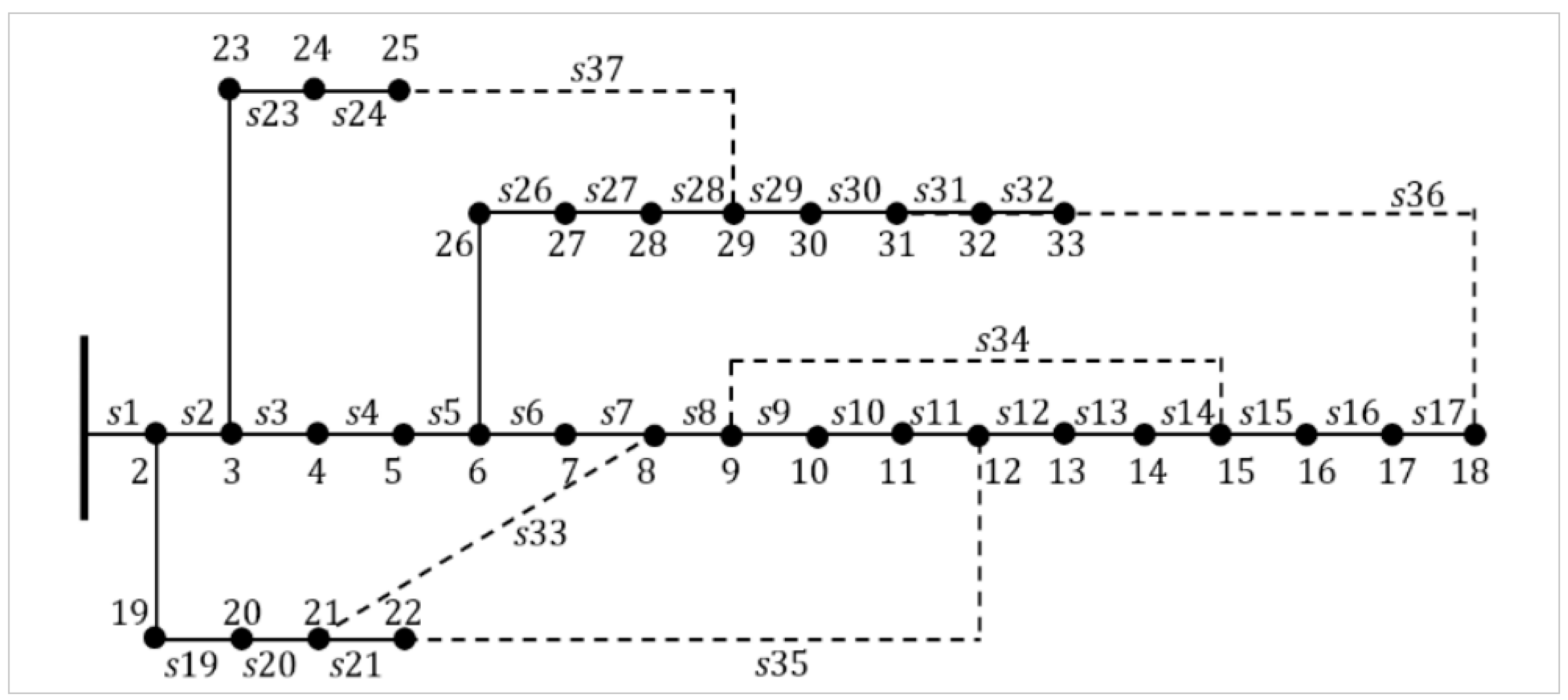
• The stochastic reconfiguration of a 33-bus electrical distribution network is performed using a multi-objective intelligent framework (MOIF) to minimize power losses and improve power quality and reliability indices considering the network load uncertainty using an unscented transformation (UT) [38]. Two power quality indicators, the decline in voltage sags and the system’s average RMS fluctuation frequency, are considered. Also, the average system interruption frequency index, the instantaneous average interruption frequency index, and the system average interruption frequency index are reliability indices;
• The UT is used to model the uncertainty of the network load in the stochastic reconfiguration problem. Compared with the Monte Carlo simulation (MCS) with high computational cost, the UT has low calculation time, and no assumptions are required to simplify the model,
• The number of open network switches is determined by a new improved mountaineering team-based optimization (IMTBO) algorithm and the conventional MTBO [39] is improved based on a quasi-opposition-based learning strategy [40] to avoid premature convergence;
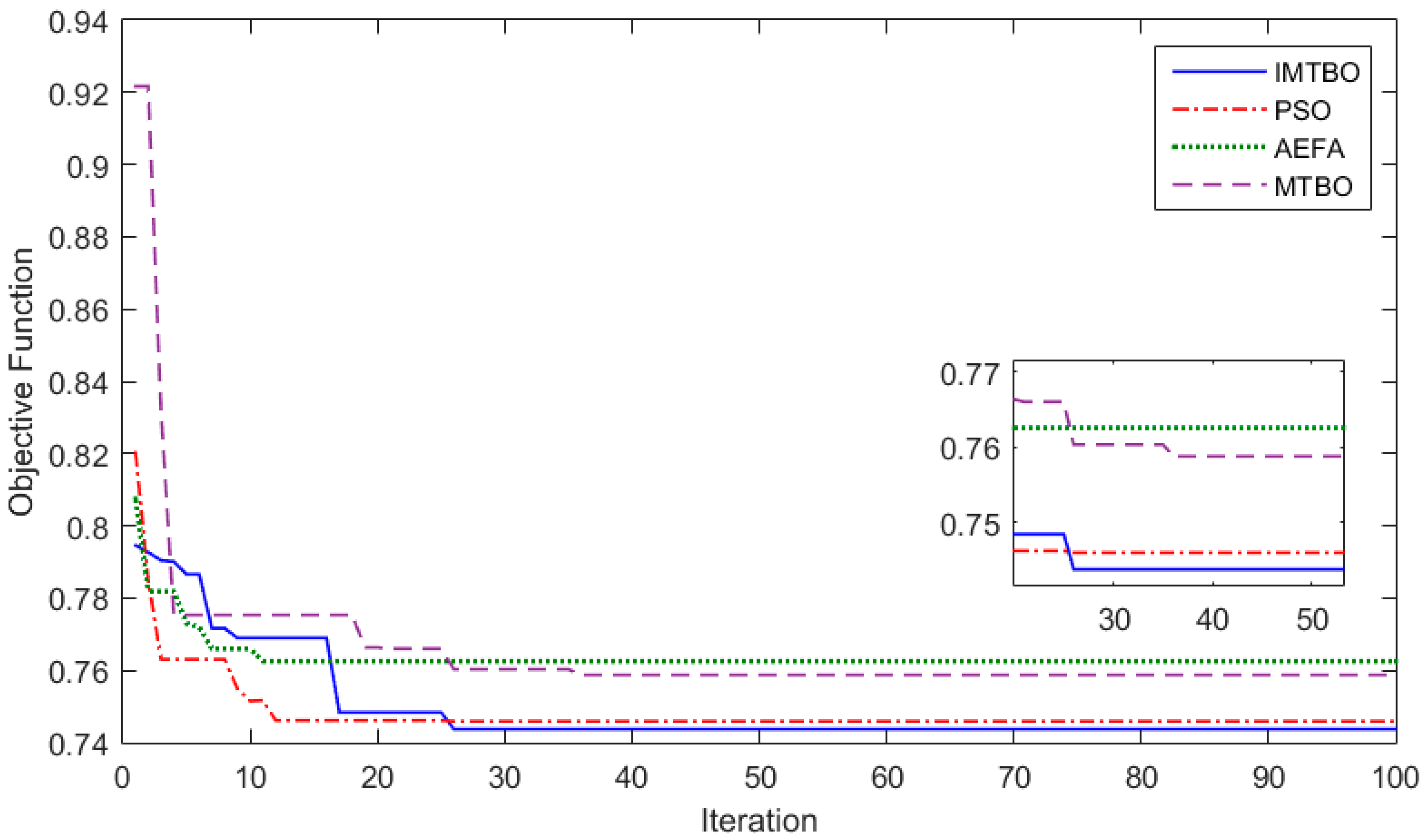
• To validate the IMTBO, it has been compared to conventional MTBO, particle swarm optimization, and the artificial electric field algorithm [41] in solving the reconfiguration problem based on the MOIF;
• Moreover, the deterministic and stochastic MOIF results are compared to evaluate the effect of the uncertainty consideration on solving the reconfiguration problem.

1.4. Paper Structure

In Section 2, the constraints for the multi-objective function and reconfiguration problem are discussed. Section 3 explains the proposed meta-heuristic strategy and implementation method for solving the optimization problem. Section 4 presents the UT approach to model the uncertainty. Section 5 describes the outcomes of the proposed methodology, and Section 6 summarizes the findings of the study.

2. Problem Statement

In this study, the MOIF is outlined for reconfiguration of the distribution network with an emphasis on decreasing electrical losses, improving power quality, and increasing reliability metrics.

2.1. Objective Function

Identification of the ideal network configuration, which is offered in this research with the MOIF for reducing power losses, increasing power quality, and improving reliability indicators, is the goal of distribution network optimization based on reconfiguration. In this research, customers are given access to power quality indicators [42,43] such as the frequency of the system’s average RMS fluctuation and the number of voltage sags ($N_{sag}$) throughout the assessment period (SARFI). Reliability indices can go by the names Average System Interrupt Frequency Index (ASIFI), Momentary Average Interrupt Frequency Index (MAIFI), and System Average Interrupt Frequency Index (SAIFI). The MOIF based on the weighted coefficients is formulated by:

$$\begin{array}{c}OF={\vartheta }_1\times \frac{P_{Loss}}{P_{Loss,max}}+{\vartheta }_2\times \frac{N_{sag}}{N_{sag,max}}+{\vartheta }_3\times \frac{SARFI}{{SARFI}_{max}}+{\vartheta }_4\times \frac{ASIFI}{{ASIFI}_{max}}+{\vartheta }_5\times \\ \frac{MAIFI}{{MAIFI}_{max}}+{\vartheta }_6\times \frac{SAIFI}{{SAIFI}_{max}}\end{array}$$

(1)

where $P_{Loss,max}$ is the maximum value of network power losses, $N_{sag,max}$ indicates the maximum number of voltage sags, ${SARFI}_{max}$ is the maximum system average RMS variation frequency, and ${ASIFI}_{max}$,${MAIFI}_{max}$, and ${SAIFI}_{max}$ are the maximum values of the ASIFI, MAIFI, and SAIFI indices. The maximum values mentioned are obtained from network load flow in base mode. Also, the set of absolute values of all weight coefficients (${\vartheta }_1, {\vartheta }_2, {\vartheta }_3, {\vartheta }_4, {\vartheta }_5, and {\vartheta }_6$) must be equal to 1.

The active power loss ($PL$) of the entire network is defined based on the total loss of all network lines as follows [42,43,44]:

$$P_{Loss}=\sum _{i=1}^{N_{branch}}{RES}_i\times {\left|{CUR}_i\right|}^2$$

(2)

where ${RES}_i$, ${CUR}_i$, and $N_{branch}$ are the resistance, the current passing through the i-th line, and the total number of network lines, respectively.

$N_{sag}$ stands for the total number of subscribers affected throughout the assessment period by all potential mistakes. Monitoring the network’s stated bus voltage (E_i) and determining the kind and location of the bus load allow one to calculate $N_{sag}$. The location of the defect in a system determines the propagation of voltage sags and the severity of voltage sags on buses located far from faults. Through fault evaluation, the sag-subjected region at each fault site is able to be found. Nevertheless, recognizing the system element which leads to significant voltage drops spreading throughout a failure is essential for improving power quality and reliability and determining the likelihood of a defect occurring. Voltage reductions are principally brought on by frequent line faults. Thus, fault analysis can identify the system lines responsible for significant slope exposure. If the faulted line fault rate with length $LL$ is $\mu$, then the determined annual quantity of line failures ($\partial$) is defined by [4,42]:

$$\partial =\sum _{i=1}^{N_{branch}}{LL}_i{\times \mu }_i$$

(3)

where $N_{sag}$ and the total amount of disruptions ($\gamma$) can be calculated by observing the magnitude of the system’s bus voltages (E_i) and distinguishing the type and location of bus load i. According to [42,43,44], the yearly $N_{sag}$ is as follows [4,20,35]:

$$N_{sag}=\sum _{i=1}^{N_{bus}}\sum _{\partial =1}^{{\partial }_{total}}\left\{\begin{array}{cc}1\hfill & \hfill if 0.1 p.u<E_i<0.9 p.u\\ 0\hfill & \hfill Otherwise\end{array}\right.$$

(4)

The $N_{sag}$ that corresponds to sensitive buses is equal to the overall number of continuous interruptions, as the majority of processes involving sensitive equipment experience lengthy interruptions. For non-sensitive loads, the overall number of disruptions annually can be calculated using the following formula [4,42]:

$$\gamma =\sum _{i=1}^{N_{bus}}\sum _{\partial =1}^{{\partial }_{total}}\left\{\begin{array}{cc}1\hfill & \hfill if E_i\le 0.1 p.u\\ 0\hfill & \hfill Otherwise\end{array}\right.$$

(5)

The disruptions emphasized in Equation (5) may be further subdivided into sustained distractions if the insensitive demand bus is the faulty bus or if it is located downward of the failure, as every one of the other buses is separated while the circuit breaker is opened to eliminate the error. The fault will be eliminated by the safety mechanism once the service is restored, so these outages can be categorized as temporary or transient. Using Equations (4) and (5), the aforementioned disruption classifications can be utilized to determine the SARFI annually along with reliability metrics.

The SARFI of the entire network can be determined using the estimated total number of voltage sags, $N_{sag}$, caused by faults. The SARFI index is presented as follows [42,43,44]:

$$SARFI=\frac{N_{sag}}{TNCS}$$

(6)

where TNCS refers to the total number of customers supplied.

The SARFI sag number could be converted into ongoing disruptions, temporary disruptions, and demand disruptions that impact the system’s accessibility. Other objective functions related to loading reliability indicators, i.e., ASIFI, MAIFI, and SAIFI, respectively, represent indicators related to loading, stable interruptions, and short-term interruptions. ASIFI can represent financial losses related to load interruptions, whereas MAIFI is used to indicate subscriber interruptions caused by protection operations. SAIFI can be used to represent the common stable interval. The defined indicators are presented below [27,42,43,44].

$$ASIFI=\frac{TQLI}{TQLS}$$

(7)

$$MAIFI=\frac{CSTI}{TNCS}$$

(8)

$$SAIFI=\frac{TCCI}{TNCS}$$

(9)

where TQLI and TQLS are interrupted and served total connected kVA demand, CSTI is the total number of customer short-term interruptions, while TCCI is the total number of customer long-term interruptions caused by each occurrence.

2.2. Constraints

During the optimization process, the problem’s objective function should be optimized within certain constraints. The following list of restrictions is provided [42,43].

2.2.1. Power Flow

$$P_i=\sum _{i=1}^{N_{bus}}{E}_i{E}_j{Y}_{ij}\cos \left({\theta }_{ij}-{\delta }_i+{\delta }_j\right)$$

(10)

$$Q_i=\sum _{i=1}^{N_{bus}}{E}_i{E}_j{Y}_{ij}\sin \left({\theta }_{ij}-{\delta }_i+{\delta }_j\right)$$

(11)

In solving the optimization problem, load distribution equations must be established in any situation. $P_i$ and ${\delta }_i$ are, respectively, the active and reactive power injected from the network to the bus, $E_i$ and δ_i are the range and angle of the i-th bus voltage, respectively, and $Y_{ij}$ and ${\theta }_{ij}$ are the range and admittance angle between the i-th and j-th nodes of the network, respectively.

2.2.2. Voltage

When addressing the optimization problem, the voltage of the network buses should not exceed the minimum and maximum values permitted.

$$E_{min}\le \left|E_i\right|{\le E}_{max}$$

(12)

where $E_{min}$ and $E_{max}$ are, respectively, the lowest and highest values of the acceptable voltage range for network buses.

2.2.3. Current

The current flowing through the network lines must not exceed the maximum allowed value and stay within the thermal range of the lines.

$$\left|{CUR}_{f,i}\right|\le {CUR}_{f,i}^{max}$$

(13)

where ${CUR}_{f,i}$ is the current passing through the i-th line of the network and ${CUR}_{f,i}^{max}$ is the maximum allowed current passing through the line.

2.2.4. Radiality Condition

Each bus in the radial network must take a single route to the main feeder since there are no loops in its configuration. The network branch matrix is created for this purpose. A matrix with the same number of rows, network lines, and columns as network buses is known as a network branch matrix. As a consequence, $\mathrm{I}nc\left({br}_{ij}\right)$ for each network line between two buses i and j is as follows [42,43]:

$$\mathrm{I}nc({br}_{ij})=\left\{\begin{array}{cc}1\hfill & \hfill nbus=i\\ -1\hfill & \hfill nbus=j\\ 0\hfill & \hfill else\end{array}\right.$$

(14)

After forming the above matrix, if its determinant is zero, the network is radial, and otherwise the matrix is non-radial. In this situation, if the condition of radiality of the network is not respected, a fine or penalty is incorporated in the value of the objective function, which is thus removed from the competition.

3. Proposed Optimizer

In this research, the MOIF for reconfiguration of the distribution network has been implemented using a new intelligent improved mountaineering team-based optimization (IMTBO) and in this section, its formulation and also the implementation method for solving the reconfiguration problem are explained.

3.1. Overview of the MTBO

3.1.1. Inspiration

The primary inspiration for the MTBO algorithm is the team’s methodical and coordinated ascent of a mountain, taking into account the possibility of natural calamities, as outlined in the stages provided below.

3.1.2. First Phase: Coordinated Mountaineering

The most seasoned member of a climbing team is always chosen to be the leader and stand in front of the group, which is analogous to the best outcome in the most recent iteration of the algorithm in optimization science. The best member of the algorithm population, or alternatively, the climbing group, fills this job. To climb the mountain peak or, alternatively, to find the finest overall solution, this person guides the best or the complete group toward the aim or objective. Members approach the group leader in the manner described below [39]:

$$X_i^{\mathrm{new}}=X_i+rand\times \left(X_{Leader}-X_i\right)$$

(15)

In a climbing team, each member is directed by both the group leader and the person in front of them as the movement is planned under the supervision of the group leader. The members are normally grouped from best to worst. The population is thought to be ranked from best to worst after each iteration of the MTBO algorithm, and each person is ranked directed by the group leader and the preceding person. Consequently, the following adjustments are made to the equation of normal motion up the mountain peak [39]:

$$X_i^{\mathrm{new}}=X_i+rand\times \left(X_{Leader}-X_i\right)+rand\times \left(X_{ii}-X_i\right)$$

(16)

In contrast, in the realm of optimization, every action occurs at random, and the phase probability is considered to be equal to Li; so, the pseudo-code of this phase is presented by [39]:

$\mathbf{i}\mathbf{f} rand<Li$

$X_i^{\mathrm{new}}=X_i+rand\times \left(X_{Leader}-X_i\right)+rand\times \left(X_{ii}-X_i\right)$

$\mathbf{e}\mathbf{n}\mathbf{d}$

3.1.3. Second Phase: Impact of Natural Catastrophes

Natural calamities often put mountaineers’ lives in peril and may keep them from reaching the summit, or, to put it another way, imprison the people between surrounding small peaks [39]. The frequency of avalanches and cliff falls is the most important factor in the MTBO algorithm. The majority of the MTBO optimization process is based on avalanches, which are a kind of natural catastrophe. The beginning of an avalanche at this point is thus more probable than it would be under other circumstances. Because of this, the critical state in the event of a randomly occurring avalanche in MTBO is seen as being similar to the worst case of the algorithm X_Worst or, alternatively, X_Avalanche. In the case of an avalanche and other catastrophes, the subject tries to flee the disaster scenario X_Worst or equivalently X_Avalanche and rescue himself utilizing the inspired equation below. To put it another way, one is freed from being constrained by a local optimum solution and is able to move toward the global optimization of the ideal solution [39].

$$X_i^{\mathrm{new}}=X_i-rand\times \left(X_{\mathrm{Avalanche}}-X_i\right)$$

(17)

It is assumed that the probability of an avalanche occurring is equal to Ai, and the pseudo-code for this phase is as follows [39]:

$\mathbf{i}\mathbf{f} rand<Ai$

$X_i^{\mathrm{new}}=X_i-rand\times \left(X_{\mathrm{Avalanche}}-X_i\right)$

$\mathbf{e}\mathbf{n}\mathbf{d}$

3.1.4. Third Phase: Concerted Action by Many People to Prevent Catastrophes

Human groups are fundamentally different from other phenomena and creatures in that they cooperate and lead one another in a highly deliberate, planned, and effective way. This kind of interpersonal teamwork is crucial in a climbing team. Therefore, in a climbing team, in the event of an emergency or someone being trapped, the whole team makes an effort to free the trapped person. Therefore, MTBO draws its inspiration from the group’s coordinated and social effort and cooperation to free the imprisoned member, whereby each member’s position is equal to the average position, or X_mean or X_Team. One is toward the X_mean or X_Team position. The following model [39] serves as a representation of this behavior:

$$X_i^{\mathrm{new}}=X_i+rand\times \left(X_{\mathrm{Team}}-X_i\right)$$

(18)

The pseudo-code for this phase is as follows [39]: The chance of rescuing a person caught in an avalanche or stuck in the best local solution is equal to Mi.

$\mathbf{i}\mathbf{f} rand<Mi$

$X_i^{\mathrm{new}}=X_i+rand\times \left(X_{\mathrm{Team}}-X_i\right)$

$\mathbf{e}\mathbf{n}\mathbf{d}$

3.1.5. Fourth Phase: Potential Demise of Members

However, it is well known that sometimes an avalanche’s strength results in the death of a member of a climbing team. It is thus probable that the climbers will die in the disaster and that none of the aforementioned precautions will be able to rescue them. The member in question is eliminated from the group at this stage of the MTBO process, and the following equation [39] is used to randomly add a new member to the group:

$$X_i^{\mathrm{new}}={X\left(X_{\max }-X_{min}\left(\right)\right)}_{min}$$

(19)

Algorithm 1 displays the general pseudo-code of the MTBO’s optimization procedure.

Algorithm 1: Mountaineering Team-Based Optimization (MTBO)

1: Setting MTBO control parameters: scaling factors including Li, Ai, and Mi, the number of iterations of the Itermax, and the number of its population NP and set the number of iterations for individuals Iter = 0; 2: Random generation of the initial population NP (I = 1, 2, …, NP); 3: $X_i={X\left(X_{\max }-X_{min}\left(\right)\right)}_{min}$; 4: Assessing the level of physical fitness of each individual; 5: while the i till maximum no of iterations Itermax do 6: Setting the number of iterations Iter = Iter + 1; 7: for i = 1 to NP do 8: $\mathrm{Selecting} \mathrm{the} \mathrm{numbers} X_{Leader}$$, X_{ii}$$, X_{\mathrm{Avalanche}}$; 9: $\mathit{i}\mathit{f} rand<Li$ 10: $X_i^{\mathrm{new}}=X_i+rand\times \left(X_{Leader}-X_i\right)+rand\times \left(X_{ii}-X_i\right)$ 11: $\mathit{e}\mathit{l}\mathit{s}\mathit{e} \mathit{i}\mathit{f} rand<Ai$ 12: $X_i^{\mathrm{new}}=X_i-rand\times \left(X_{\mathrm{Avalanche}}-X_i\right)$ 13: $\mathit{e}\mathit{l}\mathit{s}\mathit{e} \mathit{i}\mathit{f} rand<Mi$; 14: $X_i^{\mathrm{new}}=X_i+rand\times \left(X_{\mathrm{Team}}-X_i\right)$ 15: else 16: $X_i^{\mathrm{new}}={X\left(X_{\max }-X_{min}\left(\right)\right)}_{min}$; 17: end if 18: if $f\left(X_i^{\mathrm{new}}\right)<f\left(X_i\right)$ 19: $X_i$$=X_i^{\mathrm{new}}$$\mathrm{and} f\left(X_i\right)$$=f\left(X_i^{\mathrm{new}}\right)$; 20: end if 21: if $f\left(X_i\right)<f\left(X_{Leader}\right)\left(\mathit{or}f\left(X_{Best}\right)\right)$ 22: $X_{Leader}\left(or{X}_{Best}\right)$$=X_i$$\mathrm{and} f\left(X_{Leader}\right)\left(\mathit{or}f\left(X_{Best}\right)\right)$$=f\left(X_i\right)$; 23: end if 24: end for 25: end while Return the best solution is obtained via MTBO: $X_{Leader}$$\mathrm{or} X_{Best}$

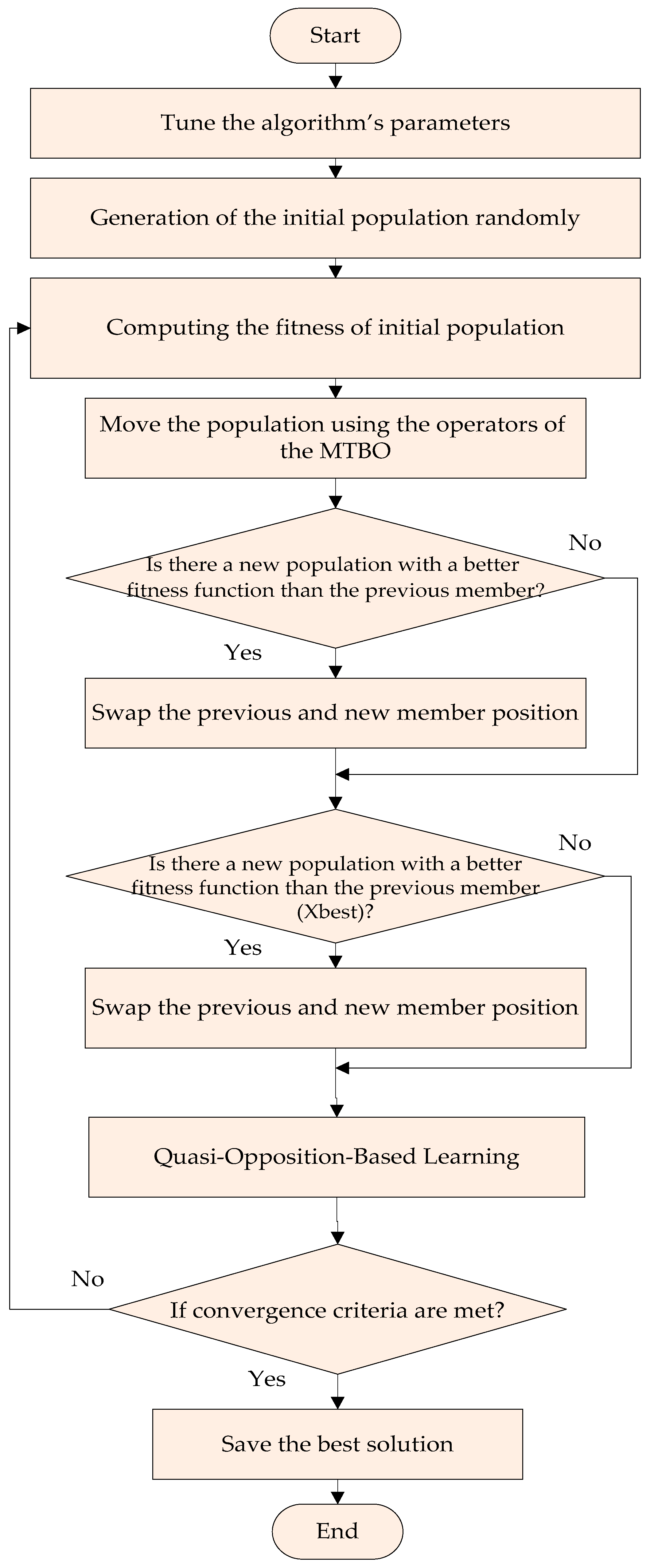
3.2. Overview of the Improved MTBO (IMTBO)

Using quasi-opposition-based learning (QOBL) [40], an observing status is stated and evaluated at each iteration in order to avoid the suggested approach becoming locked in locally optimal solutions. There are several subsequent stages involved. First, a distance constant is established between the mean and the optimal solution [40]:

$$\phi =\sqrt{\sum _{j=1}^n{(X_{\mathrm{ave},\mathrm{j}}-X_{\mathrm{best},\mathrm{j}})}^2}$$

(20)

The minimal value of the distance under the constant criterion is then determined [40]:

$${\phi }^{min}=\frac{15}{{10}^{(Iter/Itermax)}}$$

(21)

Subsequently, the monitoring condition is evaluated. If D_c < D_cmin, QOBL is used to expand the variety of the population and increase the convergence range of the algorithm. A portion of the evaluation points are considered at random, and based on this, the opposite evaluation points are produced, as well as evaluated concurrently. The fitness level of the original test points and the quasi-opposite test points are then computed and ranked ascendingly, and the initial NP solutions for the descending leadership motion and the trending leadership motion are selected. To preserve the stochastic nature of IMTBO, a quasi-opposite answer is randomly generated from the center of the search space ($X_{CS}$) and the mirrored position of every point of the test ($X_{MP}$):

$${\mathrm{X}}_{\mathrm{i},\mathrm{j}}^{\mathrm{q}}=\left\{\begin{array}{c}{X}_{CS}+rand\left(\right)\times \left(X_{MP}-X_{CS}\right), if X_{MP}>X_{CS},\\ X_{MP}+rand\left(\right)\times \left(X_{CS}-X_{MP}\right), Otherwise\\ i=1,2,\dots , Nq\end{array}\right.$$

(22)

$$X_{CS}=\frac{X_{max}{+X}_{max}}{2}$$

(23)

$$X_{MP}=X_{max}{+X}_{max}-X_{i,j}$$

(24)

where Nq is the total amount of randomly determined test points for the generation of opposite test points, which in this study has been configured to be 5.

Figure 1 depicts the flowchart of the IMTBO in the optimization process.

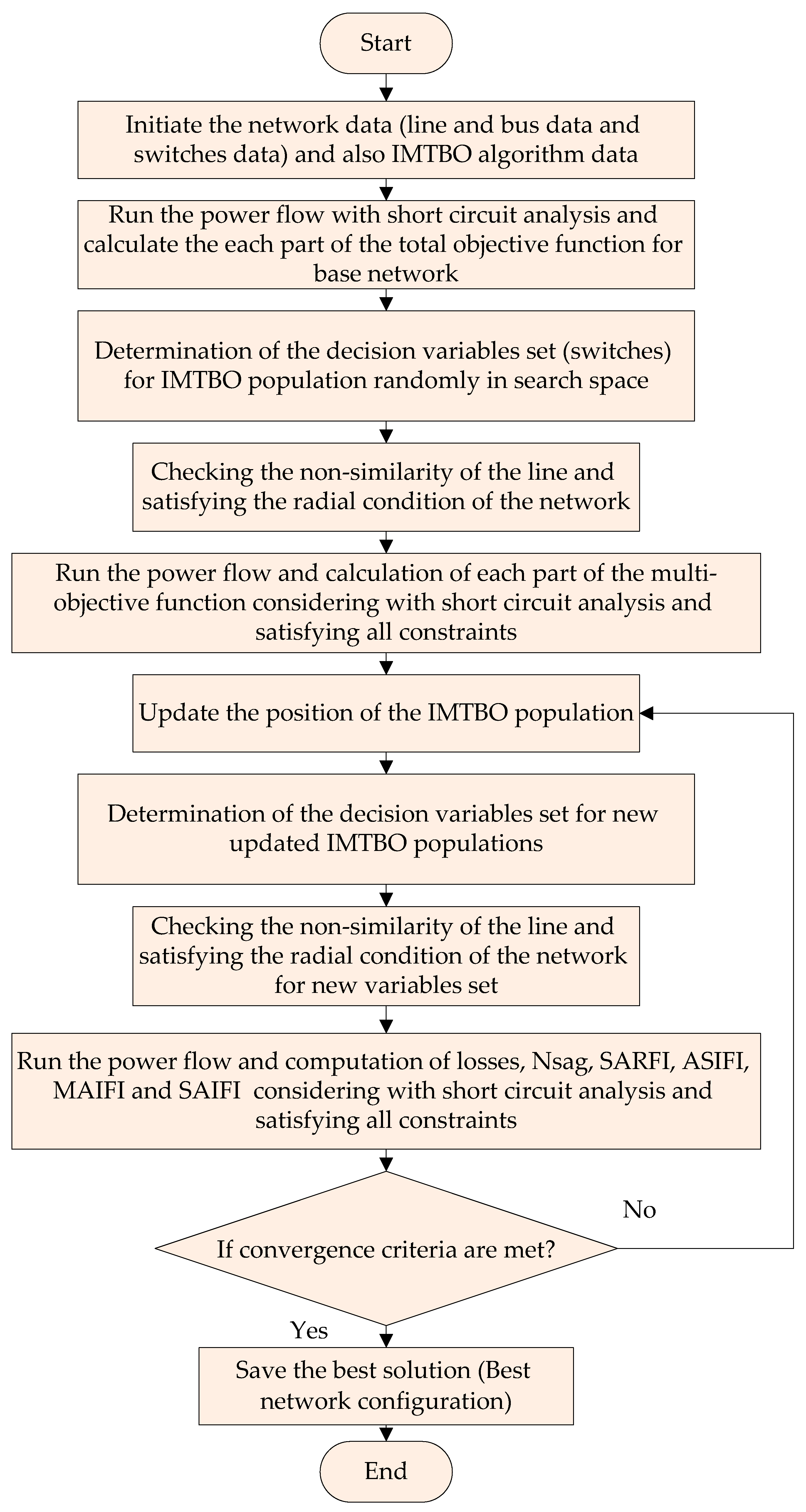
3.3. Implementation of the IMTBO

The reconfiguration of the distribution network may be completed by modifying the preset state of the tie lines, depending on the defined goal functions and constraints. For each modification to a network’s design, the $N_{sag}$, SARFI, ASIFI, MAIFI, SAIFI, and $P_{Loss}$ indices are computed in Matlab using a short-circuit evaluation and the stable-state power flow method. The network reconfiguration modifies the distribution feeders’ structural organization by modifying ties and sectioning switches’ open/closed status. By actuating a switch that connects the two feeders, a feeder can be partially or completely met by an alternative feeder. For maintaining radial structures, the sectionalizing switch must be deactivated. In distribution networks, network reconfiguration is frequently employed to minimize network losses, regulate demands, and increase voltage fluctuations. The reconfiguration is additionally useful to mitigate voltage sag minimization in the network by increasing the line impedance in failure duration. Whenever a fault occurs at certain system buses, the voltage on a few system buses may fluctuate. Consequently, the power quality and dependability of the system may be impacted by defects in the weak area. The primary objective of network reconfiguration is to reduce $N_{sag}$ and reliability indices by isolating the vulnerable area from the primary power source. To avoid increasing system-wide line losses, network reconfiguration should be restricted. There must be a balance between the rise in branch losses and the enhancement of the power quality and dependability of the network. Therefore, optimization techniques are required to find an architecture that can achieve both a small number of voltage dips and a suitable quantity of power loss.

The implementation phases of IMTBO to solve the network reconfiguration problem are depicted in Figure 2. Shown here are the reconfiguration problem’s implementation steps. Under typical conditions, the network is radial. The number of network lines should be one less than the total amount of network buses, as the network must be radial. Nevertheless, the network contains communication connections that are typically open and external to the circuit. Therefore, if you take into account the quantity of network buses n and the quantity of network lines m, you must always have m = n − 1, which stands for the active lines of the distribution network. The number of network lines that must be removed from the circuit in order to maintain the network’s radial state must be determined by the optimization method, and this number must be equal to the number of optimization variables. To preserve the network’s radial requirements, five lines must be eliminated from the circuit in the typical 33-bus network, where there are 33 buses and a total of 37 lines. This will result in five optimization variables for the n_var optimization problem. After the candidate lines to be removed from the circuit by cutting them off have been identified, it is required to examine the distribution network’s restrictions. Proposed lines for deletion must be two-by-two, and line numbers should not be duplicated. If this condition is not satisfied, the associated objective function will be severely penalized and eliminated from the optimization. After confirming the constraints of the radial network, the problem’s objective functions are studied. After removing the load from the network with the revised distribution structure, the amount of power loss is then computed. In the following, the network voltage drop has been calculated so that the number of weak buses can be identified and $N_{sag}$ may be calculated. Afterward, criteria and indicators for network dependability will be calculated. After calculating the value of the objective function corresponding to each set of optimization variables, including open network switches, all sets of responses were ranked by the objective function values, from lowest to highest. If we have reached the maximum number of allowable repetitions of the problem, the search and optimization are halted; otherwise, the optimization continues.

4. Uncertainty Modeling Based on the UT

In the problem outlined in Equations (1)–(23), uncertainties include the generation of photovoltaic and wind energy as well as the network demand. In this work, the unknown parameters are modeled via the UT technique [38]. The UT is capable of modeling uncertainty and decision-making hazards well. It was created with the idea that approximating a distribution of probabilities is simpler than approximating a consequence or transformation of an arbitrary nonlinear function [38]. The UT’s fundamental idea is the approximation of the PDF by a collection of chosen points known as sigma points and corresponding weights [38]. A weighting of these sigma points will yield metrics on the mean, variance, and other aspects of mapping moments. Low sample size requirements and simplicity of use are benefits of the UT. The parameter n, which is assigned a value of three in this study, denotes the size of the input vector for uncertainty (U) in this method. Additionally, 2n + 1 probabilities are generated. Computation time is significantly decreased because no scenario reduction strategy is used unlike the Monte Carlo simulation due to small set of possibilities. Y = f(x), where $y\in R^r$ is the uncertain output vector and includes r elements, and $x\in R^n$ is the uncertain input vector, denotes the problem with its uncertain, nonlinear, and stochastic nature. By ${\mu }_x$ and ${\sigma }_x$, the mean and covariance of x are displayed. The symmetric and asymmetric portions of x are used to determine the variance and covariance of uncertainty, respectively. The UT method’s application tries to determine the outcomes’ mean and covariance quantities, or ${\mu }_y$ and ${\sigma }_y$ [38]. The steps of UT implementation are as follows [38]:

-

Step 1: Choose 2n + 1 samples from the uncertain input data:

$$x_0={\mu }_x$$

(25)

$$x_s={\mu }_x\pm \sqrt{\frac{n}{1-W^0}\times {\sigma }_X},\hspace{0.17em}\hspace{0.17em}\hspace{0.17em}\forall s=1,2,\dots ,n$$

(26)

where W⁰ is the weight of the mean value ${\mu }_x$.

-

Step 2: Assess the weighting factor of individual sample points:

$$W_0=W_0$$

(27)

$$W_s=\frac{1-W^0}{2n},\hspace{0.17em}\hspace{0.17em}\hspace{0.17em}\forall s=1,2,\dots ,n$$

(28)

$$W_{s+n}=\frac{1-W^0}{2n},\hspace{0.17em}\hspace{0.17em}\hspace{0.17em}\forall s+n=n+1,n+2,\dots ,2n$$

(29)

$${\displaystyle \sum _{s=1}^n{W}_s}=1$$

(30)

-

Step 3: Sample 2n + 1 points to the nonlinear function to obtain output samples as per Equation (31).

$$y_S=f(x_s)$$

(31)

-

Step 4: Assess ${\mu }_y$ and ${\sigma }_y$ of the output variable θ.

$${\mu }_y={\displaystyle \sum _{s=1}^n{W}_s}{\theta }_s$$

(32)

$${\sigma }_y={\displaystyle \sum _{s=1}^n{W}_s(}{\theta }_s-{\mu }_y)-{({\theta }_s-{\mu }_y)}^T$$

(33)

5. Results and Discussions

The IMTBO method is used to simulate the MOIF for reconfiguration of the distribution network in this segment with the goal of reducing power losses and improving the indicators of power quality and distribution network reliability. The proposed strategy is implemented on the IEEE 33-bus standard distribution network (Figure 3). A total of 33 buses and 37 branches make up this network, which is fed by a 12.6 kV transmission network. Five communication switches between buses 8–21, 9–15, 12–22, 18–33, and 25–29, as well as lines 33 to 37, may be used to alter the network topology in the case of unexpected events or disruptions. The 33-bus network’s load and lines, as well as the lines’ outage rates, the network’s customer count, and also the reliability calculation requirements are all covered by the data that have been taken from references [45,46]. The balance of all loads and voltages is taken for granted in the simulation for the best reconfiguration. The primary post is not where the problem originates, and the dependability of each load point within a subscriber group is assessed. When evaluating dependability, the voltage sag problem affects all industrial loads. The superiority of the IMTBO is compared with the conventional MTBO, particle swarm optimization (PSO), and the artificial electric field algorithm (AEFA). For a fair comparison of the population size, the maximum number of iterations and repetitions for each algorithm are set to 50, 100, and 25, respectively, and the parameters of the MTBO, PSO, and AEFA algorithms are regarded as the regulatory parameters provided by their authors in the articles, as shown in

Table 1. Adjustment parameters of different algorithms.

Algorithm	Parameter
MTBO	--
PSO [32]	C1 = C2 = 2 and W: Linear decline from 0.9 to 0.1
AEFA [33,34]	Initial value used in Coulomb’s constant (K0) = 100

. The number of optimization variables equals the number of switchable lines, which is five lines. In addition, line number one, which is the connection line to the main network and the main feeder, cannot be removed or altered; therefore, the optimization variables can be adjusted from line number 2 to line number 37. The proposed methodology is implemented in Matlab 2020b environment with a personal computer with core i7, 3.1 GHz, and 1 TB.

To evaluate the effectiveness of the proposed procedure, different cases are provided as follows:

Case (1) Distribution network without reconfiguration.

Case (2) Reconfiguration to minimize power losses in addition to improving power quality.

Case (3) Reconfiguration with the aim of minimizing power losses in addition to improving reliability.

Case (4) Reconfiguration to minimize power losses and improve power quality and reliability.

Case (5) Reconfiguration to minimize power losses and improve power quality and reliability considering uncertainties.

5.1. Results of the Base Network (Case 1)

In this section, the results of power flow and fault analysis are presented to evaluate the performance of the distribution network of 33 buses before optimal reconfiguration. Except for the main post, fault analysis simulation has been done in all buses. For the basic network, the values of $P_{Loss}$, $N_{sag}$, SARFI, SAIFI, ASIFI, and MAIFI are 202.68 kW, 16,104, 8.2331, 1.3614, 2.3508, and 4.6479, respectively, which are given in

Table 2. Loss values and indicators of power quality and reliability for the base mode 33-bus network (Case 1).

Item	Base Network
Opened Switches	33, 34, 35, 36, 37
$P_{Loss}$ (kW)	202.68
$N_{sag}$	16,104
$SARFI$	8.2331
$ASIFI$	2.3508
$MAIFI$	4.6479
$SAIFI$	1.3614
$OF$	1

. Lines 33, 34, 35, 36, and 37 are open network switches or tie lines.

The simulation of short circuit fault in all buses except for the main post is done to determine the weak area or the bus that causes the voltage sag in the network. The number of voltage sags of the network buses caused by the LLL three phase fault is shown in Figure 4.

It is possible to identify buses with the potential to impair power quality and reliability. Buses 6, 7, 23, 24, and 29 are the most sensitive buses to the propagation of voltage drop in the entire network, and bus 29 affects more than the rest of the network buses. Figure 5 shows the network voltage profile in normal conditions and with the LLL fault in bus 29.

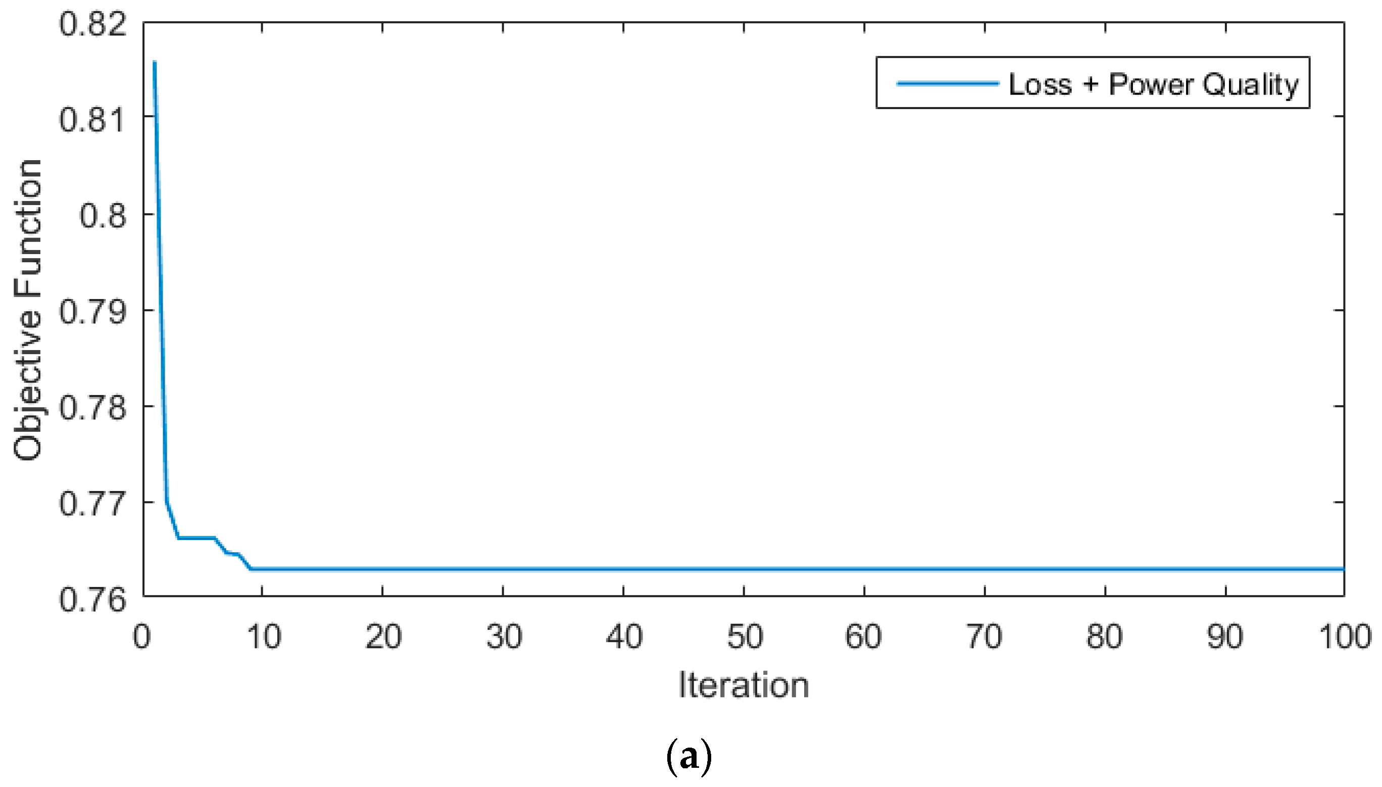
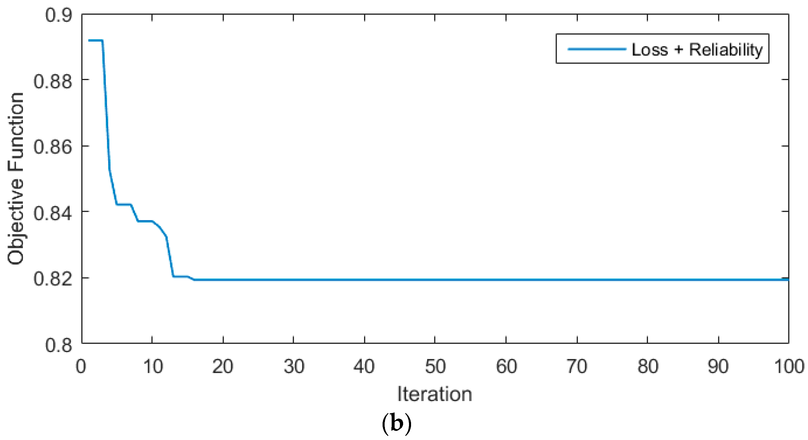
5.2. Results of Dual-Objective Reconfiguration (Cases 2 and 3)

This part uses the IMTBO method to simulate a dual-objective reconfiguration of the distribution network with the goals of reducing power losses and power quality indicators (case 2) as well as power losses and reliability indicators (case 3). The convergence curve of the IMTBO in solving two different problems is shown in Figure 6. It can be seen that the IMTBO algorithm has converged with few iterations with different objective functions.

The simulated outcomes of the MOIF for reconfiguration of the distribution network using the IMTBO to reduce power losses are shown in

Table 3. Results of solving cases 2 and 3 using the IMTBO.

Item/Method	Base Network	Loss + Power Quality (Case 2)	Loss + Reliability (Case 3)
Opened Switches	33, 34, 35, 36, 37	7, 9, 14, 28, 32	7, 8, 9, 16, 28
$P_{Loss}$ (kW)	202.68	149.9782	153.5122
$N_{sag}$	16,104	10,680	11,016
$SARFI$	8.23	5.46	5.63
$ASIFI$	2.35	2.33	2.11
$MAIFI$	4.64	3.95	2.98
$SAIFI$	1.36	1.36	1.33
$OF$	1	0.7629	0.81934

. For case 1, the IMTBO has determined the optimal arrangement of the network by leaving lines 7, 9, 14, 28, and 32 open, and for case 2 by opening lines 7, 8, 9, 16, and 28. Comparison of the results of cases 2 and 3 shows that case 1 has obtained better power quality indicators, i.e., lower $N_{sag}$ and SARFI values, compared to case 2. Also, the comparison of the results of cases 2 and 3 shows that case 2 has obtained better reliability indices, i.e., lower ASIFI, MAIFI, and SAIFI values compared to case 2. The amount of power loss is also lower in case 3 compared to case 2. The results showed that each of cases 2 and 3 improved the network performance to the maximum from their point of view, and from another point of view, the amount of improvement was not significant, in other words, a suitable compromise between all loss targets and indicators of power quality and reliability was not established.

5.3. Results of MOIF for Reconfiguration (Case 4)

In this study, using the proposed optimization algorithm (also user experience) and considering the sum of weighted coefficients to be equal to 1, simulations are performed for a set of different weighted coefficients. The optimal values of different objectives such as P_Loss, N_sag, SARFI, ASIFI, MAIFI, and SAIFI are obtained at 0.2, 0.2, 0.15, 0.15, 0.15, and 0.15, respectively.

This part also uses the IMTBO to simulate the consequences of the MOIF for reconfiguration of the distribution network with the goal of decreasing power losses, power quality indicators, and reliability indicators (case 4). In this section, the IMTBO performance is compared with conventional MTBO, PSO, and AEFA algorithms. The convergence curve of different algorithms in solving case 4 is shown in Figure 7. It can be seen that the IMTBO algorithm has a lower convergence tolerance compared to other algorithms and the optimal solution is obtained with a lower objective function value, which indicates its better performance compared to other algorithms.

The optimization results along with various reliability and power loss indices are presented in

Table 4. Numerical results of solving case 4 using different algorithms.

Item/Method	Base Network	IMTBO	PSO	AEFA	MTBO
Opened Switches	33, 34, 35, 36, 37	7, 9, 14, 28, 32	7, 10, 14, 28, 32	7, 9, 14, 17, 28	9, 28, 32, 33, 34
$P_{Loss}$ (kW)	202.68	139.97	166.94	146.28	144.77
$N_{sag}$	16,104	10,680	11,520	10,848	10,848
$SARFI$	8.23	5.46	5.88	5.54	5.54
$ASIFI$	2.35	2.19	2.35	2.19	2.16
$MAIFI$	4.64	2.57	2.99	2.95	2.81
$SAIFI$	1.36	1.35	1.36	1.39	1.37
$OF$	1	0.74372	0.74594	0.76256	0.75876
$CT \left(\mathrm{s}\right)$	-	142.36	144.11	148.57	150.68

Note: CT is calculation time.

. As can be seen, the IMTBO has obtained a lower value of the objective function compared to other methods. Therefore, the IMTBO algorithm has shown better overall performance in improving each of the objectives compared to the PSO, AEFA, and conventional MTBO methods. However, the obtained value of some objectives has exceeded its allowed value by conventional MTBO, PSO, and AEFA methods (numbers in red). The amount of power loss by each of the IMTBO, PSO, AEFA, and conventional MTBO methods is 139.97 kW, 166.94 kW, 146.28 kW, and 144.77 kW, respectively, and $N_{sag}$ value is 10,680, 11,520, 10,848, and 10,848, respectively, SARFI value is obtained 5.46, 5.88, 5.54 and 5.54, respectively, ASIFI value is 2.19, 2.35, 2.19, and 2.16, respectively, MAIFI value is 2.57, 2.99, 2.95, and 2.81, respectively, and SAIFI value is 1.36, 1.36, 1.39, and 1.37, respectively. The results showed that the IMTBO method has shown better performance in improving all objectives compared to other methods with a higher convergence rate (minimum iteration number and minimum calculation time (CT)).

In this study, the buses that have a voltage lower than 0.95 p.u are defined as weak buses. The number of weak buses for the base network without reconfiguration is 21, which after reconfiguration has decreased to 8, i.e., it has decreased by 61.9%. The $N_{sag}$ criterion in the basic state is equal to 16,104 points, which has decreased to 10,680 with optimization based on the IMTBO method, i.e. by 33.68%. The active power loss of the network has also decreased by 30.94% from 202.68 kW to 139.97 kW. The SARFI power quality index has also decreased by 33.68% from 8.23 to 5.46. In addition, the ASIFI and MAIFI indices decreased by 6.43% and 44.57%, respectively, from 2.35 and 4.64 to 2.19 and 2.57, respectively. Significant financial losses may come from the interruption of heavy loads due to poor network power quality and low reliability, hence these improvements in power quality and reliability indicators are highly desirable. The SAIFI index has changed significantly and reached 1.35 from 1.36 and decreased by 0.74%.

The IMTBO efficiently generates the optimal reconfiguration solution in several iterations. Power quality and network reliability have improved significantly, despite a slight improvement in the system’s SAIFI benchmark. Figure 8 shows the number of network bus drops after solving case 3 by IMTBO after the LLL fault in different locations. The voltage sag performance of different network buses has improved significantly compared to the base state.

The performance of the proposed method is compared with various previous studies in

Table 5. Results comparison of the proposed method with previous studies.

Item/Method	IMTBO	MFO [47]	EGA [48]	SSA [49]	BWOA [50]
Opened Switches	7, 9, 14, 28, 32	7, 10, 14, 28, 36	10, 13, 16, 28, 33	7, 14, 30, 35, 37	7, 9, 14, 28, 32
$P_{Loss}$ (kW)	139.97	142.42	164.41	115.73	139.98
$SAIFI$	1.35	--	2.158	2.2716	--

. In [47], the network reconfiguration is presented to minimize the power losses and energy not supplied using a moth-flame optimizer. In [48], the reconfiguration of the distribution network is performed for minimizing the losses, energy not supplied, and SAIFI using an enhanced GA (EGA). In [49], a salp swarm algorithm is used to configure the 33-bus network to minimize losses and SAIFI. In [50], the reconfiguration of the distribution network is developed using the black widow optimization algorithm to minimize the losses and improve the voltage stability.

The studies conducted in the field of network reconfiguration clearly show that the studies have not provided a comprehensive objective function based on power loss and power quality and reliability indicators, and only the objective function of power loss is common among all studies. Therefore, our paper considers different objectives to achieve a real reconfiguration. As can be seen, our method achieves a lower amount of power loss as well as a lower SAIFI, which indicates the superiority of the proposed IMTBO method to improve the network performance based on the reconfiguration.

5.4. Analysis of Different Cases

In

Table 6. The single- and multi-objective functions results based on the MOIF.

Objective Function	Lines	${\mathit{N}}_{\mathit{s}\mathit{a}\mathit{g}}$	${\mathit{P}}_{\mathit{L}\mathit{o}\mathit{s}\mathit{s}}$ (kW)	SARFI	ASIFI	MAIFI	SAIFI
Base network (Case 1)	33, 34, 35, 36, 37	16,104	202.68	8.23	2.35	4.64	1.36
$N_{sag}$	6, 9, 14, 16, 28	10,512	154.81	5.39	2.20	2.96	1.06
$P_{Loss}$	7, 9, 14, 17, 28	10,848	139.95	5.54	2.09	2.95	1.39
$SARFI$	6, 10, 15, 27, 34	10,760	163.63	5.37	2.20	2.99	1.35
$ASIFI$	10, 13, 16, 28, 33	12,696	161.58	6.49	1.99	3.01	1.08
$MAIFI$	6, 10, 13, 26, 31	11,832	174.14	6.04	2.52	2.56	1.06
$SAIFI$	6, 9, 14, 17, 24	11,208	184.60	5.73	2.50	3.23	1.05
Case 2	7, 9, 14, 28, 32	10,680	149.97	5.48	2.33	3.95	1.36
Case 3	7, 8, 9, 16, 28	11,016	153.51	5.63	2.11	2.98	1.33
Case 4	7, 9, 14, 28, 32	10,680	139.97	5.46	2.19	2.57	1.35

, the results of single-objective reconfiguration with different objective functions are presented. The IMTBO method has been run 30 times for each objective function to evaluate the optimal reconfiguration performance. The best optimization results with different objective functions until the last iteration of optimization for each single-objective optimization are presented in Table 6. The $N_{sag}$ objective function is the most appropriate objective function to improve power quality. The results showed that the best value of each goal in single-objective optimization is provided for the same goal. In addition, the results of Table 6 show that in single-objective optimizations some indicators are even weakened compared to their base state. The results show that when all the indicators of loss, power quality, and reliability are considered as the objective function, a better compromise has been made between all the objectives, and in general, according to Table 3 and Table 4, a lower objective function value has been obtained.

5.5. Results of MOIF for Reconfiguration Considering Demand Uncertainty (Case 5)

In this section, results of the MOIF for distribution network reconfiguration considering the network demand uncertainty are presented in

Table 7. The results comparison of deterministic and stochastic MOIF for network reconfiguration.

Case	Lines	${\mathit{N}}_{\mathit{s}\mathit{a}\mathit{g}}$	${\mathit{P}}_{\mathit{L}\mathit{o}\mathit{s}\mathit{s}}$	SARFI	ASIFI	MAIFI	SAIFI
Deterministic (Without uncertainty, Case 4)	7, 9, 14, 28, 32	10,680	139.97	5.46	2.19	2.57	1.35
Stochastic (With uncertainty, Case 5)	7, 10, 28, 32, 34	11,256 5.39	150.64 7.62	5.75 5.31	2.24 2.28	2.74 6.61	1.37 1.48

and compared with the deterministic results (Case 4). The results showed that considering the uncertainty of the network load demand in the stochastic reconfiguration model, in addition to the increased network power losses, the power quality and reliability indicators were also weakened. Therefore, it is necessary to include the uncertainty of the load in the detailed network reconfiguration for the decision of the network operators. The results showed that in the stochastic model, taking into account the uncertainty of the load, the amount of power loss 7.62%, the number of voltage sag 5.39%, the SARFI index 5.31%, and each of the reliability indices of ASIFI, MAIFI, and SAIFI, 2.28%, 6.61%, and 1.48%, respectively, have increased compared to the deterministic reconfiguration model. The IMTBO method determined the optimal network configuration by opening switches 7, 10, 28, 32, and 34. In the stochastic reconfiguration model, the UT approach has a low calculation time compared to the Monte Carlo simulation and no need to assumptions to simplify the model.

6. Conclusions

In this study, the network’s MOIF for stochastic reconfiguration was investigated to minimize power losses and enhance the reliability and power quality indices considering demand uncertainty using the UT. The new IMTBO was utilized to find the network’s optimal configuration to satisfy operational requirements, and preserve network radiality. Additionally, the MOIF was resolved using the PSO, AEFA, and conventional MTBO techniques, and the outcomes were compared and investigated to validate the IMTBO. To find the location or bus responsible for the network’s voltage sag, a simulation of short-circuit faults was performed on all buses, excluding the main post.

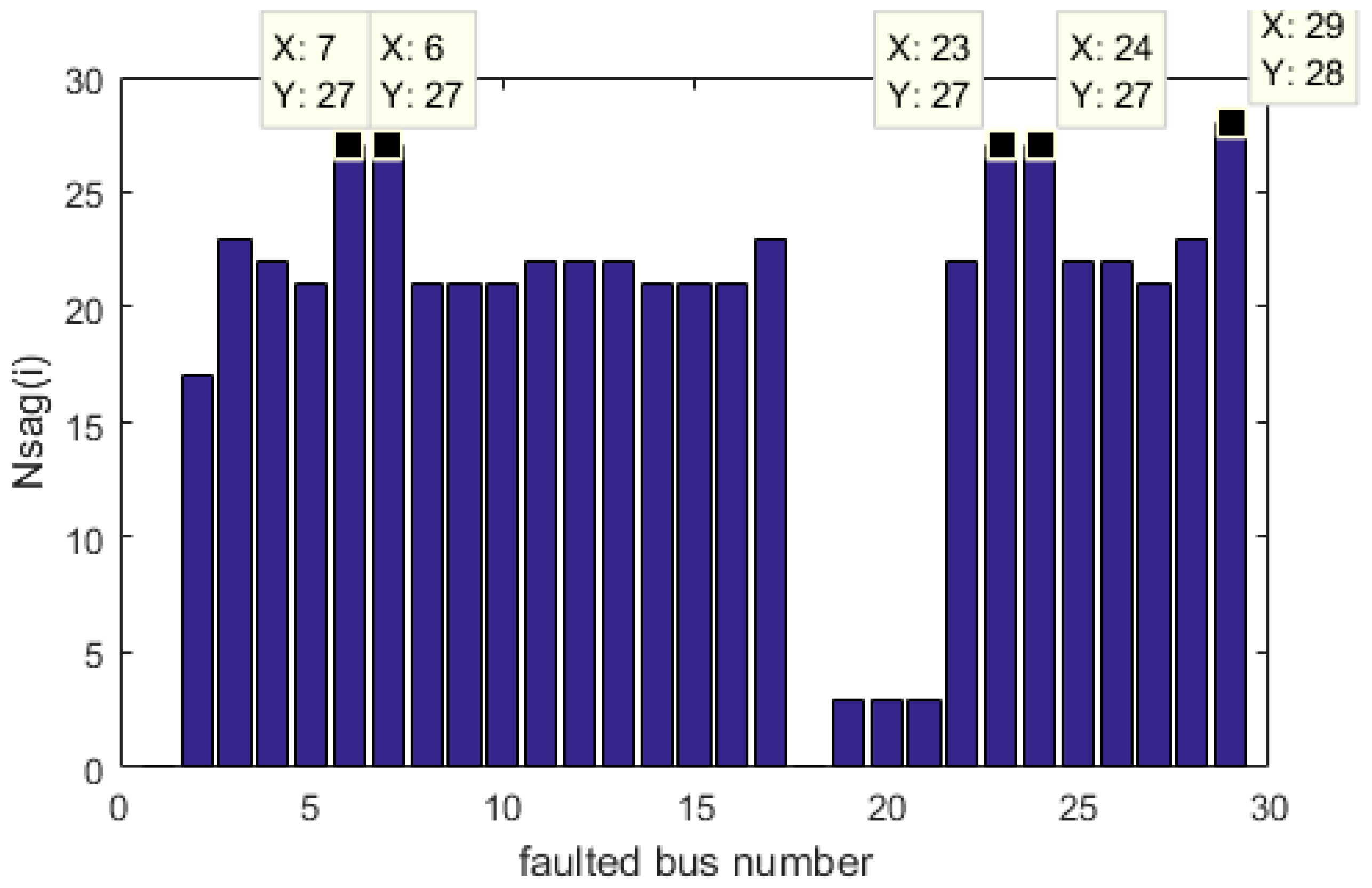
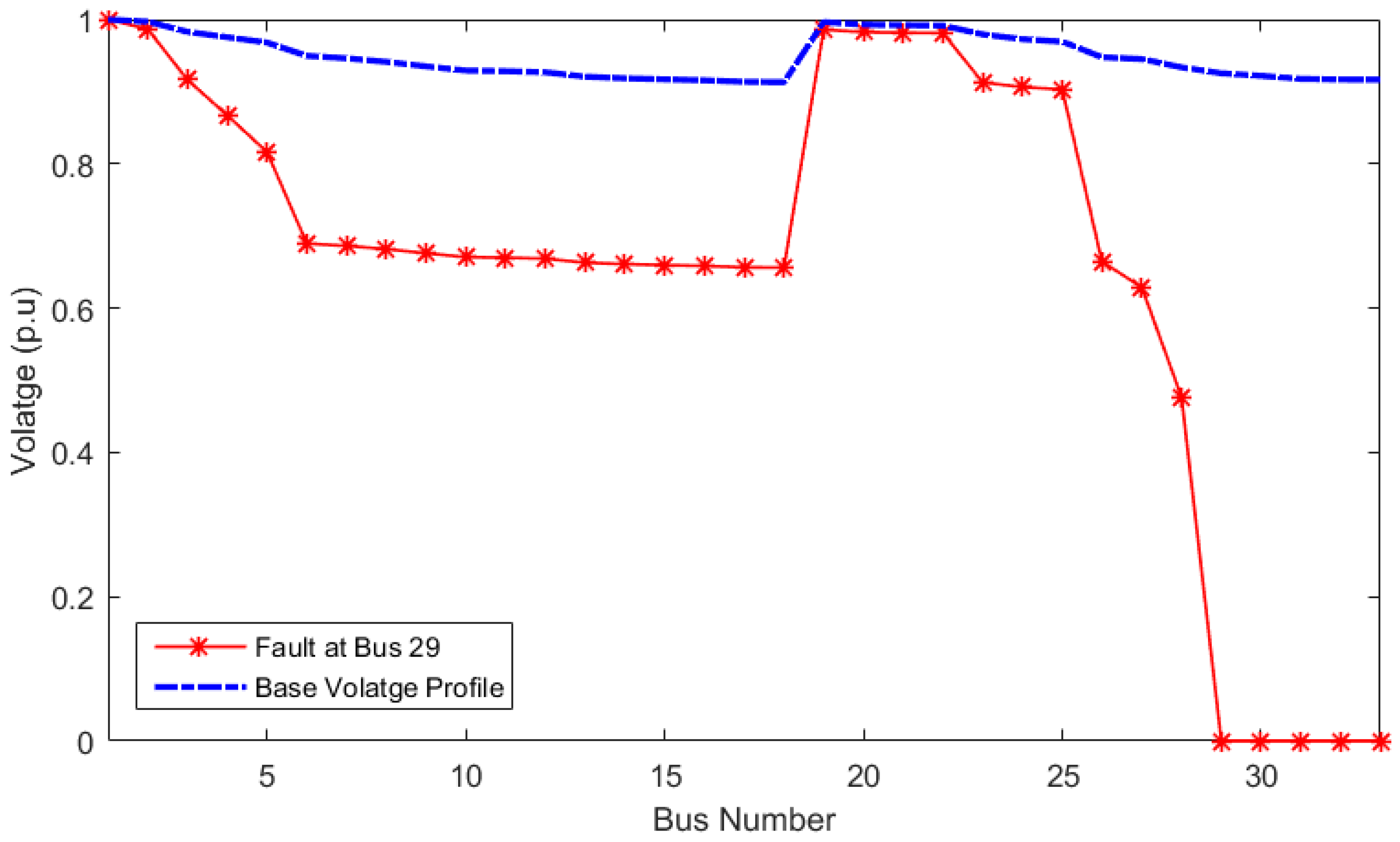
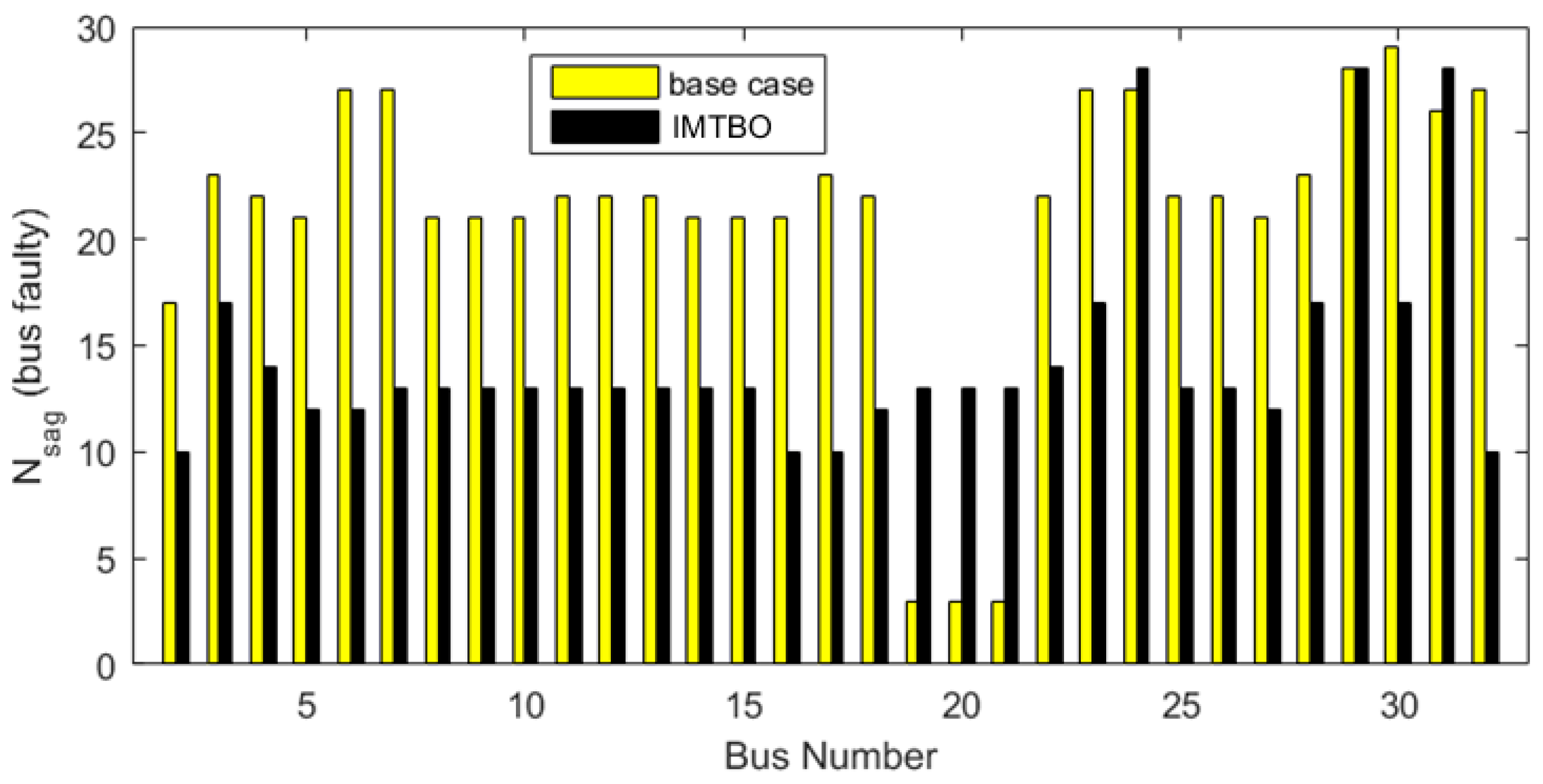
• According to the results, buses 6, 7, 23, 24, and 29 were the most sensitive to the spread of voltage sag across the entire network, with bus 29 affecting the plurality of network buses;
• In terms of power quality and reliability indicators, as well as an objective function value, simulation results demonstrated that the IMTBO optimization method was preferable to PSO, AEFA, and conventional MTBO;
• The results showed that the success of the proposed MOIF reduced active losses by 30.94%, improved the SARFI index by 33.68%, and enhanced the ASIFI and MAIFI indices by 6.43% and 44.57%, respectively;
• The MOIF for reconfiguration has enhanced network performance in terms of power quality and reliability in comparison to single-objective reconfiguration, whereas single-objective reconfiguration cannot produce a desirable compromise between all objectives. In addition, the superior efficacy of the proposed IMTBO-based method compared to Refs. [42,43,44,45] is validated;
• Moreover, the results of the stochastic reconfiguration based on the UT, clearly showed that the losses were increased, and also the power quality and reliability indices were weakened compared to the deterministic MOIF without uncertainty. The results illustrated that considering the demand uncertainty allows the network operator to make accurate decisions and to be aware of the network’s optimal configuration. The results showed that the UT was able to model the uncertainty simply with a low number of sampling points.

References

1. Wang, Y.; Ma, H.; Xiao, X.; Wang, Y.; Zhang, Y.; Wang, H. Harmonic State Estimation for Distribution Networks based on Multi-Measurement Data. IEEE Trans. Power Deliv. 2023, 38, 2311–2325. [Google Scholar] [CrossRef]
2. Naderipour, A.; Abdullah, A.; Marzbali, M.H.; Nowdeh, S.A. An improved corona-virus herd immunity optimizer algorithm for network reconfiguration based on fuzzy multi-criteria approach. Expert Syst. Appl. 2022, 187, 115914. [Google Scholar] [CrossRef] [PubMed]
3. Kanwar, N.; Gupta, N.; Niazi, K.R.; Swarnkar, A.; Abdelaziz, A.Y. Day-Ahead Optimal Scheduling of Distributed Resources and Network Reconfiguration Under Uncertain Environment. Electr. Power Compon. Syst. 2020, 48, 1945–1954. [Google Scholar] [CrossRef]
4. Xu, S.; Huang, W.; Huang, D.; Chen, H.; Chai, Y.; Ma, M.; Zheng, W.X. A Reduced-Order Observer-Based Method for Simultaneous Diagnosis of Open-Switch and Current Sensor Faults of a Grid-Tied NPC Inverter. IEEE Trans. Power Electron. 2023, 38, 9019–9032. [Google Scholar] [CrossRef]
5. Soliman, M.; Abdelaziz, A.Y.; El-Hassani, R.M. Distribution power system reconfiguration using whale optimization algorithm. Int. J. Appl. Power Eng. (IJAPE) 2020, 9, 48–57. [Google Scholar] [CrossRef]
6. Wang, Y.; He, H.-S.; Xiao, X.-Y.; Li, S.-Y.; Chen, Y.-Z.; Ma, H.-X. Multi-Stage Voltage Sag State Estimation Using Event-Deduction Model Corresponding to EF, EG, and EP. IEEE Trans. Power Deliv. 2022, 38, 797–811. [Google Scholar] [CrossRef]
7. Zhu, L.; Li, Z.; Hou, K. Effect of radical scavenger on electrical tree in cross-linked polyethylene with large harmonic superimposed DC voltage. High Volt. 2022. [Google Scholar] [CrossRef]
8. Xu, S.; Huang, W.; Wang, H.; Zheng, W.; Wang, J.; Chai, Y.; Ma, M. A Simultaneous Diagnosis Method for Power Switch and Current Sensor Faults in Grid-Connected Three-Level NPC Inverters. IEEE Trans. Power Electron. 2022, 38, 1104–1118. [Google Scholar] [CrossRef]
9. Wang, Z.; Zhao, D.; Guan, Y. Flexible-constrained time-variant hybrid reliability-based design optimization. Struct. Multidiscip. Optim. 2023, 66, 89. [Google Scholar] [CrossRef]
10. Alanazi, A.; Alanazi, M.; Nowdeh, S.A.; Abdelaziz, A.Y.; El-Shahat, A. An optimal sizing framework for autonomous photovoltaic/hydrokinetic/hydrogen energy system considering cost, reliability and forced outage rate using horse herd optimization. Energy Rep. 2022, 8, 7154–7175. [Google Scholar] [CrossRef]
11. Cao, B.; Zhao, J.; Gu, Y.; Ling, Y.; Ma, X. Applying graph-based differential grouping for multiobjective large-scale optimization. Swarm Evol. Comput. 2019, 53, 100626. [Google Scholar] [CrossRef]
12. Cao, B.; Dong, W.; Lv, Z.; Gu, Y.; Singh, S.; Kumar, P. Hybrid Microgrid Many-Objective Sizing Optimization With Fuzzy Decision. IEEE Trans. Fuzzy Syst. 2020, 28, 2702–2710. [Google Scholar] [CrossRef]
13. Naderipour, A.; Nowdeh, S.A.; Saftjani, P.B.; Abdul-Malek, Z.; Bin Mustafa, M.W.; Kamyab, H.; Davoudkhani, I.F. Deterministic and probabilistic multi-objective placement and sizing of wind renewable energy sources using improved spotted hyena optimizer. J. Clean. Prod. 2020, 286, 124941. [Google Scholar] [CrossRef]
14. Zhang, J.; Kong, D.; He, Y.; Fu, X.; Zhao, X.; Yao, G.; Teng, F.; Qin, Y. Bi-layer energy optimal scheduling of regional integrated energy system considering variable correlations. Int. J. Electr. Power Energy Syst. 2023, 148, 108840. [Google Scholar] [CrossRef]
15. Diaaeldin, I.; Aleem, S.A.; El-Rafei, A.; Abdelaziz, A.; Zobaa, A.F. Optimal Network Reconfiguration in Active Distribution Networks with Soft Open Points and Distributed Generation. Energies 2019, 12, 4172. [Google Scholar] [CrossRef]
16. Dekhandji, F.Z.; Baali, H.; Recioui, A. Optimal Placement of DGs in the Distribution Networks using an Analytical Approach. In Proceedings of the 2022 13th International Renewable Energy Congress (IREC), Hammamet, Tunisia, 13–15 December 2022; pp. 1–6. [Google Scholar] [CrossRef]
17. Swaminathan, D.; Rajagopalan, A.; Montoya, O.D.; Arul, S.; Grisales-Noreña, L.F. Distribution Network Reconfiguration Based on Hybrid Golden Flower Algorithm for Smart Cities Evolution. Energies 2023, 16, 2454. [Google Scholar] [CrossRef]
18. Dias Santos, J.; Marques, F.; Garcés Negrete, L.P.; Andrêa Brigatto, G.A.; López-Lezama, J.M.; Muñoz-Galeano, N. A novel solution method for the distribution network reconfiguration problem based on a search mechanism enhancement of the improved harmony search algorithm. Energies 2022, 12, 2083. [Google Scholar] [CrossRef]
19. Diaaeldin, I.M.; Aleem, S.H.E.A.; El-Rafei, A.; Abdelaziz, A.Y.; Zobaa, A.F. A Novel Graphically-Based Network Reconfiguration for Power Loss Minimization in Large Distribution Systems. Mathematics 2019, 7, 1182. [Google Scholar] [CrossRef]
20. Jakus, D.; Čađenović, R.; Vasilj, J.; Sarajčev, P. Optimal Reconfiguration of Distribution Networks Using Hybrid Heuristic-Genetic Algorithm. Energies 2020, 13, 1544. [Google Scholar] [CrossRef]
21. Alanazi, A.; Alanazi, M.; Nowdeh, S.A.; Abdelaziz, A.Y.; Abu-Siada, A. Stochastic-metaheuristic model for multi-criteria allocation of wind energy resources in distribution network using improved equilibrium optimization algorithm. Electronics 2022, 12, 3285. [Google Scholar] [CrossRef]
22. Pereira, E.C.; Barbosa, C.H.N.R.; Vasconcelos, J.A. Distribution Network Reconfiguration Using Iterative Branch Exchange and Clustering Technique. Energies 2023, 16, 2395. [Google Scholar] [CrossRef]
23. Kahouli, O.; Alsaif, H.; Bouteraa, Y.; Ben Ali, N.; Chaabene, M. Power System Reconfiguration in Distribution Network for Improving Reliability Using Genetic Algorithm and Particle Swarm Optimization. Appl. Sci. 2021, 11, 3092. [Google Scholar] [CrossRef]
24. Quintana, E.; Inga, E. Optimal Reconfiguration of Electrical Distribution System Using Heuristic Methods with Geopositioning Constraints. Energies 2022, 15, 5317. [Google Scholar] [CrossRef]
25. Yang, M.; Li, J.; Li, J.; Yuan, X.; Xu, J. Reconfiguration Strategy for DC Distribution Network Fault Recovery Based on Hybrid Particle Swarm Optimization. Energies 2021, 14, 7145. [Google Scholar] [CrossRef]
26. Ayalew, M.; Khan, B.; Alaas, Z.M. Optimal Service Restoration Scheme for Radial Distribution Network Using Teaching Learning Based Optimization. Energies 2022, 15, 2505. [Google Scholar] [CrossRef]
27. Shareef, H.; Ibrahim, A.; Salman, N.; Mohamed, A.; Ai, W.L. Power quality and reliability enhancement in distribution systems via optimum network reconfiguration by using quantum firefly algorithm. Int. J. Electr. Power Energy Syst. 2014, 58, 160–169. [Google Scholar] [CrossRef]
28. Čađenović, R.; Jakus, D.; Sarajčev, P.; Vasilj, J. Optimal Distribution Network Reconfiguration through Integration of Cycle-Break and Genetic Algorithms. Energies 2018, 11, 1278. [Google Scholar] [CrossRef]
29. Shaheen, A.; Elsayed, A.; El-Sehiemy, R.A.; Abdelaziz, A.Y. Equilibrium optimization algorithm for network reconfiguration and distributed generation allocation in power systems. Appl. Soft Comput. 2021, 98, 106867. [Google Scholar] [CrossRef]
30. Ali, Z.M.; Diaaeldin, I.M.; El-Rafei, A.; Hasanien, H.M.; Aleem, S.H.A.; Abdelaziz, A.Y. A novel distributed generation planning algorithm via graphically-based network reconfiguration and soft open points placement using Archimedes optimization algorithm. Ain Shams Eng. J. 2021, 12, 1923–1941. [Google Scholar] [CrossRef]
31. Fathi, R.; Tousi, B.; Galvani, S. A new approach for optimal allocation of photovoltaic and wind clean energy resources in distribution networks with reconfiguration considering uncertainty based on info-gap decision theory with risk aversion strategy. J. Clean. Prod. 2021, 295, 125984. [Google Scholar] [CrossRef]
32. Azad-Farsani, E.; Sardou, I.G.; Abedini, S. Distribution Network Reconfiguration based on LMP at DG connected busses using game theory and self-adaptive FWA. Energy 2020, 215, 119146. [Google Scholar] [CrossRef]
33. Wang, X.; Liu, X.; Jian, S.; Peng, X.; Yuan, H. A distribution network reconfiguration method based on comprehensive analysis of operation scenarios in the long-term time period. Energy Rep. 2021, 7, 369–379. [Google Scholar] [CrossRef]
34. Nguyen, T.T.; Nguyen, T.T.; Nguyen, N.A.; Duong, T.L. A novel method based on coyote algorithm for simultaneous network reconfiguration and distribution generation placement. Ain Shams Eng. J. 2021, 12, 665–676. [Google Scholar] [CrossRef]
35. Anteneh, D.; Khan, B.; Mahela, O.P.; Alhelou, H.H.; Guerrero, J.M. Distribution network reliability enhancement and power loss reduction by optimal network reconfiguration. Comput. Electr. Eng. 2021, 96, 107518. [Google Scholar] [CrossRef]
36. Qu, Y.; Liu, C.C.; Xu, J.; Sun, Y.; Liao, S.; Ke, D. A global optimum flow pattern for feeder reconfiguration to minimize power losses of unbalanced distribution systems. Int. J. Electr. Power Energy Syst. 2021, 131, 107071. [Google Scholar] [CrossRef]
37. Abdelkader, M.A.; Osman, Z.H.; Elshahed, M.A. New analytical approach for simultaneous feeder reconfiguration and DG hosting allocation in radial distribution networks. Ain Shams Eng. J. 2020, 12, 1823–1837. [Google Scholar] [CrossRef]
38. Nowdeh, S.A.; Naderipour, A.; Davoudkhani, I.F.; Guerrero, J.M. Stochastic optimization–based economic design for a hybrid sustainable system of wind turbine, combined heat, and power generation, and electric and thermal storages considering uncertainty: A case study of Espoo, Finland. Renew. Sustain. Energy Rev. 2023, 183, 113440. [Google Scholar] [CrossRef]
39. Faridmehr, I.; Nehdi, M.L.; Davoudkhani, I.F.; Poolad, A. Mountaineering Team-Based Optimization: A Novel Human-Based Metaheuristic Algorithm. Mathematics 2023, 11, 1273. [Google Scholar] [CrossRef]
40. Zheng, T.; Luo, W. An Enhanced Lightning Attachment Procedure Optimization with Quasi-Opposition-Based Learning and Dimensional Search Strategies. Comput. Intell. Neurosci. 2019, 2019, 1589303. [Google Scholar] [CrossRef]
41. Anita; Yadav, A. AEFA: Artificial electric field algorithm for global optimization. Swarm Evol. Comput. 2019, 48, 93–108. [Google Scholar] [CrossRef]
42. Moghaddam, M.J.H.; Kalam, A.; Shi, J.; Nowdeh, S.A.; Gandoman, F.H.; Ahmadi, A. A New Model for Reconfiguration and Distributed Generation Allocation in Distribution Network Considering Power Quality Indices and Network Losses. IEEE Syst. J. 2020, 14, 3530–3538. [Google Scholar] [CrossRef]
43. Dovgun, V.; Temerbaev, S.; Chernyshov, M.; Novikov, V.; Boyarskaya, N.; Gracheva, E. Distributed power quality conditioning system for three-phase four-wire low voltage networks. Energies 2020, 19, 4915. [Google Scholar] [CrossRef]
44. Ch, Y.; Goswami, S.; Chatterjee, D. Effect of network reconfiguration on power quality of distribution system. Int. J. Electr. Power Energy Syst. 2016, 83, 87–95. [Google Scholar] [CrossRef]
45. Mendoza, J.; López, E.; López, M.; Coello, C.C. Microgenetic multiobjective reconfiguration algorithm considering power losses and reliability indices for medium voltage distribution network. IET Gener. Transm. Distrib. 2009, 3, 825–840. [Google Scholar] [CrossRef]
46. Ghasemi, S. Balanced and unbalanced distribution networks reconfiguration considering reliability indices. Ain Shams Eng. J. 2018, 9, 1567–1579. [Google Scholar] [CrossRef]
47. Jafar-Nowdeh, A.; Babanezhad, M.; Arabi-Nowdeh, S.; Naderipour, A.; Kamyab, H.; Abdul-Malek, Z.; Ramachandaramurthy, V.K. Meta-heuristic matrix moth–flame algorithm for optimal reconfiguration of distribution networks and placement of solar and wind renewable sources considering reliability. Environ. Technol. Innov. 2020, 20, 101118. [Google Scholar] [CrossRef]
48. Duan, D.-L.; Ling, X.-D.; Wu, X.-Y.; Zhong, B. Reconfiguration of distribution network for loss reduction and reliability improvement based on an enhanced genetic algorithm. Int. J. Electr. Power Energy Syst. 2015, 64, 88–95. [Google Scholar] [CrossRef]
49. Yan, X.; Zhang, Q. Research on Combination of Distributed Generation Placement and Dynamic Distribution Network Reconfiguration Based on MIBWOA. Sustainability 2023, 15, 9580. [Google Scholar] [CrossRef]
50. Nasser Hussain, A.; Rafa Abed, W.; Muneer Yaqoob, M. Dual Strategy of Reconfiguration with Capacitor Placement for Improvement Reliability and Power Quality in Distribution System. J. Eng. 2023, 2023, 1943535. [Google Scholar] [CrossRef]
Figure 1. The proposed IMTBO algorithm’s flowchart.
Mathematics 11 03658 g001
Figure 2. Flowchart of the proposed methodology based on IMTBO.
Mathematics 11 03658 g002
Figure 3. The IEEE 33-bus distribution network.
Mathematics 11 03658 g003
Figure 4. Number of network bus voltage sags caused by the LLL fault.
Mathematics 11 03658 g004
Figure 5. Voltage profile of bus 29 with the LLL problem and the 33-bus network under normal circumstances.
Mathematics 11 03658 g005
Figure 6. Convergence curve of IMTBO in solving the problem with different objectives (a) Case 2 and (b) Case 3.
Mathematics 11 03658 g006aMathematics 11 03658 g006b
Figure 7. Convergence characteristics of different methods in solving the problem (Case 4).
Mathematics 11 03658 g007
Figure 8. Number of network bus voltage drops using IMTBO after LLL error in different buses (Case 4).
Mathematics 11 03658 g008