Article

An Improved Strength Pareto Evolutionary Algorithm 2 with Adaptive Crossover Operator for Bi-Objective Distributed Unmanned Aerial Vehicle Delivery

School of Science, Wuhan University of Technology, Wuhan 430070, China
*
Author to whom correspondence should be addressed.
Mathematics 2023, 11(15), 3327; https://doi.org/10.3390/math11153327
Submission received: 6 July 2023 / Revised: 26 July 2023 / Accepted: 26 July 2023 / Published: 28 July 2023
(This article belongs to the Section Mathematics and Computer Science)

Abstract

:
With the development of the e-commerce industry, using UAVs (unmanned aerial vehicles) to deliver goods has become more popular in transportation systems. This delivery method can reduce labor costs and improve the distribution efficiency, and UAVs can reach places that are difficult for humans to reach. Because some goods are perishable, the quality of the delivery will have an impact on the customer satisfaction. At the same time, the delivery time should also meet the needs of customers as much as possible. Therefore, this paper takes the distribution distance and customer satisfaction as the objective functions, establishes a bi-objective dynamic programming model, and proposes an improved SPEA2 (strength Pareto evolutionary algorithm 2). The improved algorithm introduces the local search strategy, on the basis of the original algorithm. It conducts a local search for the better non-dominated solutions obtained in each iteration. The new dominated solutions and non-dominated solutions are determined, and the crossover operator is improved, so that the local search ability is improved, on the basis of ensuring its global search ability. The numerical experiment results show that the improved algorithm achieves an excellent performance in three aspects: the Pareto front, generation distance, and spacing, and would have a high application value in UAV cargo delivery and other MOPs (multi-objective optimization problems). The average spacing value of the improved algorithm is more than 20% smaller than SPEA2 + SDE (strength Pareto evolution algorithm 2–shift-based density estimation), which is the second-best algorithm. In the comparison of the average generation distance value, this number reaches 30%.

1. Introduction

With the development of the e-commerce industry, great changes have taken place in the field of logistics and delivery. In order to reduce labor costs and improve the delivery efficiency, more and more logistics companies are beginning to use UAVs (Unmanned Aerial Vehicles) to deliver goods, although the UAV logistics technology is not mature. At the same time, compared with the traditional logistics industry, it faces a series of constraints, such as air control. However, the advantages of UAV logistics systems are very significant, such as flexibility, ease of use, and operability. These qualities ensure they have a place in the future development of the logistics industry [1].
In the existing UAV delivery research, the main focus is on the shortest total path of UAV flight [2]. Although this is an important factor affecting revenue, the impact of time on UAV delivery has not been given enough attention. Generally, customers have certain requirements for the delivery time of goods. If we can deliver the goods within the time required by customers, we can obtain a higher level of satisfaction. On the other hand, more and more people are beginning to buy perishable goods, such as fruits and vegetables, through online shopping [3]. The quality of such goods at the time of delivery will greatly affect the customer satisfaction. These goods can easily decay during transportation. In some countries, the loss rate during transportation is as high as 30%, which is even more serious in underdeveloped regions [4]. This will also have a high negative impact on the local economy.
In addition, with improvements in shopping platform functions, consumers can evaluate the products they buy on a platform. If the purchased items do not meet expectations in terms of the freshness, quality, integrity, etc., the customer will give poor comments to the seller. This will greatly reduce the desire of other consumers to shop at that business. Through observing the evaluation areas of several e-commerce companies, Zhang et al. [5] found that customers are usually most concerned with the freshness, quality, and delivery efficiency of goods.
To summarize, the object of this study is to identify not only the shortest delivery distance of a UAV, but also how customer satisfaction is affected by delayed delivery, and the deterioration of perishable products. In other words, this paper studies a two-objective optimization problem. Therefore, a MOEA (multi-objective evolutionary algorithm) will be used to solve the problem. In short, this paper has the following differences from the existing research of this type. First of all, when considering customer satisfaction, the existing research is usually based on the delivery time. However, in this paper, in addition to considering this factor, we acknowledge that the customer satisfaction is also affected by the quality of the goods delivered. Secondly, we propose an improved SPEA2 (strength Pareto evolutionary algorithm 2) to solve the problem. Through a local search and improved crossover operator, the improved algorithm avoids the defects of easy-to-fall-into local optimization and a slow convergence speed. The relationship between customer satisfaction and distance cost is expressed through the Pareto frontier, which is selected and judged by the sellers themselves. Finally, the concept of convergence distance is proposed, to judge the convergence speed of the algorithm.
Compared with existing similar studies, this paper makes the following contributions:
  • This paper establishes a bi-objective model to solve the UAV delivery problem. The previous way of thinking, which only considered the total cost of transportation, is changed, to face this type of problem from a multi-objective perspective, and the effect of the freshness of perishable products is taken into account when calculating the customer satisfaction.
  • An improved SPEA2 is proposed in this paper. Considering that SPEA2 itself performs well in global searching, this paper conducts local searching for the points with higher adaptation after each iteration, meaning that it takes both the global and local searching ability into account. In addition, the crossover operator is also improved, to increase the convergence speed of the algorithm, and avoid falling into local optimality.
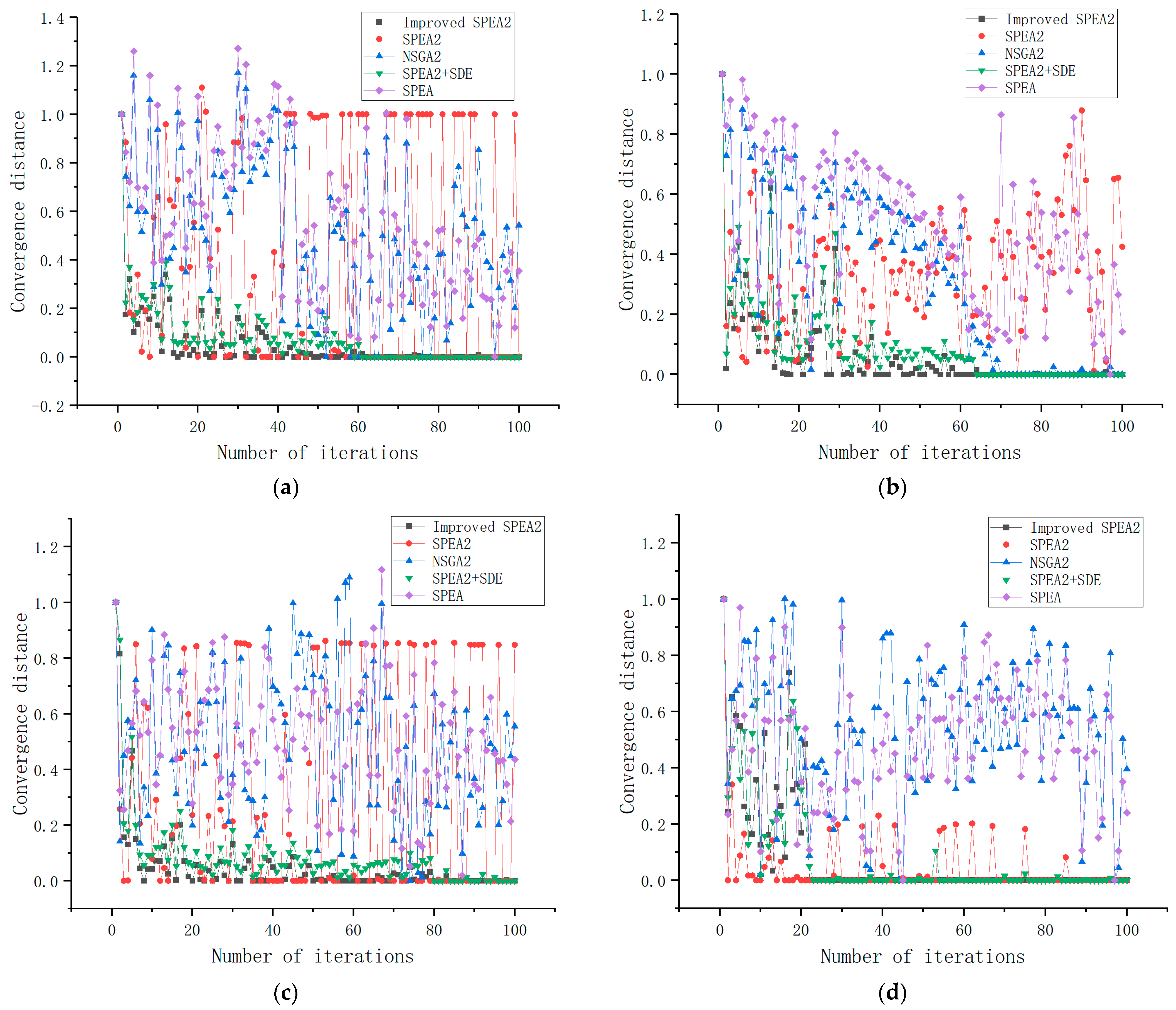
  • The concept of convergence distance is proposed in this paper. The convergence speed of the algorithm is judged by calculating the distance between the experimental results and the theoretical optimal results.
The other chapters of this article are as follows. In the second chapter, the relevant background of the MOEA, memetic algorithms, and UAV delivery is summarized, which provides a basis for the algorithm improvement and model construction. The third chapter constructs and analyzes the UAV delivery model and its constraint function. The fourth chapter improves the SPEA2. Based on the original algorithm, a local search strategy and new crossover operator are introduced, to improve the algorithm. The fifth chapter compares the improved algorithm with other MOEAs, under nine benchmarks [6], and verifies the superiority, stability, and convergence of the improved algorithm. Then, the parameters are determined through experiments, and the improved algorithm is used to solve the model. The improved algorithm can take into account both the distance cost and time cost, and is better than other MOEAs. The last chapter summarizes the work of the paper, points out the advantages and disadvantages, and proposes the focus of future work.

2. Related Work

2.1. Background of the MOEA

So far, there have been more than 20 methods proposed to solve MOPs (multi-objective optimization problems) in operational research. Most of them follow a fixed pattern. They use specific tech MOPs in multiple single-objective optimization problems. In this way, an optimal solution can be easily obtained. However, the solution of MOPs is not a single solution, but a solution set, and all the points in the set must meet the conditions [7]. In addition, results obtained by same method may be different. This is because the solution is closely related to “decision-makers”. Different decision-makers focus on different goals.
The evolutionary algorithm is a common method of solving optimization problems. Its advantage is that it can deal with a very large search space, which is in line with the characteristics of MOPs. Therefore, many scholars consider using an evolutionary algorithm to optimize multiple objectives. The MOEA is derived from this. Compared with traditional methods, it can obtain multiple optimal solutions in one run [8].
The research history of the MOEA is not long. Due to the different main characteristics of the algorithm [9], its evolution can be considered to comprise two stages [10]:
(1)
First-generation MOEA
In 1985, Schaffer [11] improved the single-objective genetic algorithm, and proposed Vega, which was the first real MOEA. Goldberg first introduced Pareto into the genetic algorithm in 1989, which had a significant and far-reaching impact on the development of multi-objective optimization. Subsequently, MOEAs sprung up: in 1993, the MOGA (multi-objective genetic algorithm) was proposed by Fonseca and Fleming [12]; in 1994, Srinivas et al. [13] proposed the NSGA (non-dominated sorting genetic algorithm) and improved the selection operator; in the same year, Horn et al. [14] proposed the NPGA (niched Pareto genetic algorithm). In brief, the first generation MOEA is characterized by the use of the selection strategy based on the Pareto level, and the diversity maintenance strategy based on the fitness sharing mechanism [15].
(2)
Second-generation MOEA
Since entering the 21st century, with the rapid development of the related technologies, many classical algorithms have been proposed. Zitzler et al. proposed the SPEA (strength Pareto evolution algorithm) [16] and the SPEA2 [17]. The SPEA2 is one of the representative classical algorithms of the second generation. The algorithm adds the external archive set, and maintains the scale of the external archive set through the clustering and pruning methods. In addition, the concept of Pareto dominance is also introduced into the assignment calculation of the population individual fitness. Deb et al. proposed the classical algorithm NSGA-II (non-dominated sorting genetic algorithm-II) [18] in the second generation MOEA. The algorithm uses better accounting strategies, according to various Pareto-dominated frontiers, which reduces the running time of the algorithm. The other major MOEAs also include the PAES (Pareto archived evolution strategy) [19] and the NPGA2 (niched Pareto genetic algorithm 2) [20], the PESA (Pareto envelope-based selection algorithm) [21] and the PESA-II (Pareto envelope-based selection algorithm-II) [22]. The remarkable feature of the second-generation MOEA is the elite individual preservation mechanism.
(3)
Classification of MOEA
According to different environmental selection strategies, there are four types of current MOEAs [23,24,25]: (a) dominance-based; (b) indicator-based; (c) decomposition-based; and (d) others.
The SPEA2 is a force-based approach among many MOEAs. After each iteration, a series of dominant and non-dominant solutions will be obtained, and then the applicability of the solution will be judged according to the quantity of its dominating non-dominant solutions. In addition, an external file will be set to store the non-dominant solution. In each iteration, these solutions are reevaluated, and the external archive is updated. Whether the solution will be used depends on its strength after each update [26]. Finally, the solutions in the external file, and the non-dominated solutions in the population make up the optimal solution set.

2.2. Background of Memetic Algorithms

Memetic algorithms (MAs) were first introduced by Moscato et al. [27,28]. Memetics represents the unity of cultural evolution, which can spread, and show local enhancement. Therefore, these algorithms are mostly used to improve the local search ability of genetic algorithms [29].
Initially, MAs focused on genetic algorithms. Later, they were extended to improve the local search capability of evolutionary strategies. They can also be used to improve swarm-based and other population-based metaheuristics [30]. In addition, several types of local search strategies have been adopted, such as simulated annealing [31], tabu search [32], and pattern search [33], to improve the solution refinement capabilities of the swarm-based metaheuristics.
One of the reasons for the increasing popularity of MAs is their performance on high-dimensional and non-differentiable search spaces, and their enhanced exploitation capabilities [34]. Therefore, many papers have proposed, improved, or used MAs for discrete, continuous, constrained, multi-objective, and other classes of optimization problems [34].

2.3. Background of Goods Delivery

As people’s consumption of perishable products increases, the research on the delivery of perishable goods is also increasing steadily. First of all, we will review the literature on single-objective problems in this field.
Tarantilis and Kiranoudis [35] solved the problem of fresh milk distribution with heterogeneous fleets in 2001. They proposed an algorithm based on the threshold acceptance, but the goal was to minimize the distance. Rabbani et al. [36] considered the loss of freshness in their research, and included it in the total cost. However, it was still a single-target problem, which could be solved by a genetic algorithm. Alvarez and Cordeau et al. [37] regarded the corrosion of goods as the inventory cost, which was one of the factors affecting the total profit, and then used the branch-cut algorithm to maximize the total profit. Liang et al. [38] wanted to use multiple distribution tools to reduce the transportation distance, so they considered the delivery of different perishable goods. When considering the decay of goods, they also considered the impact of the temperature and humidity on the goods. However, they did not study the impact of goods decay on customer satisfaction. Compared with the usual targets in the past, Meneghetti and Ceschia [39], when studying such problems, instead considered the fuel consumption of the transportation vehicles. Because the goods needed to be refrigerated during the distribution process, the fuel consumption would be increased. Based on this point, they conducted research to increase profits.
As mentioned above, these are all goods distribution and delivery problems with only a single goal, and the goal is usually an economic one; for example, the shortest distance, the largest total revenue, and the lowest fuel consumption. Although researchers have taken into account the impact of goods decay on earnings, this is only one factor. When it is considered as a single goal, a multi-objective optimization framework can provide new ideas and better solutions. Therefore, we will review the multi-objective research in this area.
Wang et al. [40] took the total cost and the number of vehicles as the two objectives of their study, and established a multi-database model. In addition to solving the model, they also added the service time, as a third goal, to the model, and built a three-goal model. When setting targets, Tirkolaee and Aydin [41] focused on gas emissions and job opportunities, in addition to costs. In their research, whether perishable goods deteriorated was an uncertain parameter, and they used the fuzzy method to solve it. In addition, in the delivery of perishables, the customer satisfaction will also have a great impact on revenue. This concept was first proposed by Cardozo [42]. He believed that customers would buy the products they were satisfied with again, and consider other products from the business. At the same time, customers would also recommend the products they were satisfied with to other customers, affecting further purchases. Rahami and Armand [43] took customer satisfaction into account when establishing a dual-objective model for perishable products. In their model, a delayed delivery would reduce the customer satisfaction, and the customer satisfaction could be expressed in this way. In the research of Wang et al. [44], time and freshness were two factors that affected the customer satisfaction. The researchers set priorities for customers’ needs, and solved this problem by modifying the priority function.
As far as we know, few studies have taken the transportation cost and customer satisfaction as the two objectives for goods delivery. In previous studies, the customer satisfaction was usually determined by the customer waiting time. However, when perishable goods are delivered, their quality has a great impact on the customer satisfaction [45]. This study establishes a model of the impact of the perishable product quality and the time window on the customer satisfaction. The details will be described in the next chapter.

3. Model Building

3.1. Problem Statement and Assumptions

In the problems studied in this paper, the supplier must achieve two goals; namely, reducing the distance cost of delivering the products, and improving the customer satisfaction. The customer satisfaction is affected by the quality of the product, and by the waiting time of the customer at the time of delivery. Therefore, each customer’s needs, and the expected delivery time, must be known. On this premise, we must study how to reduce costs and improve customer satisfaction at the same time. To solve this problem, the following assumptions must be made first [46]:
(1)
The number of UAVs in the distribution center is enough to complete all tasks.
(2)
Each customer can only submit one order, and can only be served once by a UAV.
(3)
The same order cannot be completed by multiple UAVs; that is, the cargo demand of any order cannot exceed the maximum load capacity of a single UAV.
(4)
All the products are fresh before delivery, and the quality decreases during transportation.
The goods in this paper are perishable products. Therefore, the relationship between the degree of product decay and the time must be known. These products can be divided into two categories: products with a fixed period of validity, such as beverages and biscuits, and products with an indefinite period of validity, such as fruits and vegetables. For the first type of product, the deterioration degree is easy to calculate, but the deterioration degree of the other type of product is affected by many factors. Labuza [47] has discovered that the deterioration of the second type of product conforms to the zero-order reaction function.
This paper takes fresh vegetables as the products to be delivered. Their deterioration follows the zero-order reaction function q t = q 0 φ t , where q t is the quality at time t and q 0 is the initial quality. φ is the deterioration rate of this type of vegetable, obtained by Wang and Li as 0.0216/h [48].

3.2. Notations

The mathematical symbols used in the model are as follows:
Sets:
O : Set of distribution centers
P : Set of UAVs
C : Set of delivery points
A S : Set of all points
Parameters:
V : The average velocity of a UAV
V k : Unit distance cost of a UAV k , k P
Q k : Maximum load of a UAV k , k P
D k : Maximum mileage of a UAV k , k P
t i j : Time from point i to point j , i ,   j A S , i j
c i j : Distance from point i to point j , i ,   j A S , i j
d i : Demand of customer i , i C
b j : Pickup volume from distribution center j , j O
q k j L : Load of UAV k leaving point j , k P , j A S
φ : The deteriorate rate, 0.0216/h
φ i k : The deterioration degree of the goods transported by UAV k , received by customer i , i C , k P
L T i : The latest delivery time that customer i can accept, i C
Decision variables:
X i j k = 1         if   UAV   k   flies   from   point   i   to   point   j 0         otherwise
Y i k = 1       if   UAV   k   delivers   goods   to   customer   i 0       otherwise
T k i A : The time of UAV k arriving at point i
Z i k = 1         T k i A > L T i 0       T k i A L T i

3.3. The Mathematic Model

3.3.1. Objective Function

(1)
Minimize distance cost:
f 1 = m i n i A S j S k P X i j k V k c i j
(2)
Maximize customer satisfaction:
f 2 = m i n k P i C φ i k d i / i C d i + k P i C Z i k T k i A L T i / i C L T i
The objective function (1) minimizes the distance cost, which is a common objective function in such problems, and is still one of the objectives in this paper. The ultimate goal of the objective function (2) is to maximize the customer satisfaction, which is affected by the degree of goods deterioration and the delivery time. The deterioration degree of goods follows the zero-order reaction function. The more serious the deterioration degree, the lower the customer satisfaction. At the same time, the goods delivered within the time required by customers will not affect the customer satisfaction but, once that time is exceeded, the time penalty will be triggered, and the customer satisfaction will be reduced. Therefore, the objective function (2) minimizes these two variables, to maximize the customer satisfaction.

3.3.2. Constraint Function

Formula (3) means that the UAV must leave after completing the order of customer j . Equation (4) restricts each customer to being served only once. Constraint (5) requires that the goods transported by the UAV each time cannot exceed its maximum load. Equations (6) and (7) are the calculation methods for the transportation time and the deterioration of goods, respectively. Formula (8) means that the pickup volume of the UAV must be equal to the customer’s demand. Constraint (9) is the load constraint of the UAV [49,50].
i A S X i j k l A S X j l k = 0
k P Y i k = 1
i C Y i k d i Q k
t i j = c i j / V
φ i k = q 0 φ T k i A Y i k
i C j O X i j k b j = j O l C X j l k d i
i A S j A S c i j X i j k D k

3.4. Model Analysis

When modeling the UAV delivery problem, scholars usually only consider the distance cost. In general, the shorter the distance, the lower the delivery cost. Therefore, the method that can obtain the shortest distance is often adopted. However, many goods need to be delivered at the specified time, such as fresh food and medicine. The delivery being too late may lead to food decay, or the best time to treat patients being missed. Fresh vegetables and fruits, especially, will inevitably decay during transportation. These consequences will lead to a reduction in customer satisfaction, thus affecting the long-term profits of businesses. Therefore, while focusing on the distance cost, this paper establishes a bi-objective model, with customer satisfaction as the object.
Through the study of the two objective functions, it is found that there is a negative correlation between them. To maximize the customer satisfaction, it is necessary to avoid the deterioration of goods as much as possible. This will make the transportation distance longer, and the distance cost higher. On the contrary, when the shortest route is used for transportation, some customers will wait for a long time. This will not only trigger the time penalty, but also lead to the serious deterioration of the goods. Therefore, we considered using the MOEA, which is more conducive to solving bi-objective problems with a negative correlation.

4. SPEA2 and Its Improvement

4.1. Overview of SPEA2

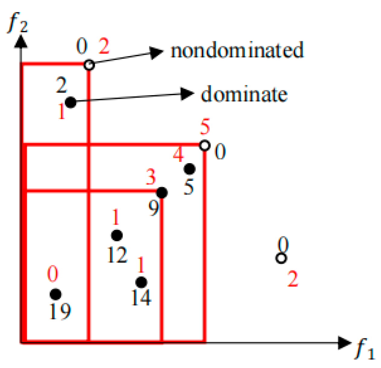
4.1.1. Pareto Optimal Solution Theory

In MOPs, the multiple objectives to be optimized are usually in conflict. Therefore, such problems do not have a specific optimal solution, and cannot be solved directly. Only by optimizing as many objectives as possible, can a compromise solution set be obtained, which is the Pareto optimal solution set. Then, according to different requirements, people can choose the desired solution from this set. Broadly speaking, there is no better solution than the Pareto solution set, so it is the optimal solution set [51].
MOPs can usually be expressed as Equation (10) [52]:
Max   or   min   F x = f 1 x , f 2 x , , f m x       s .   t .   x Ω
The decision variables are represented by x . By choosing the correct value of x , the ideal solution of the optimization problem can be obtained. The solution in the Pareto solution set cannot result in all the objectives reaching the optimal value but, when one objective is determined, the Pareto solution can allow the other objectives to reach the optimal value. Therefore, when choosing the optimal solution, we can only consider the Pareto solution set. Pareto solutions will degrade other objective functions when improving one objective function, which is completely consistent with the characteristics of MOPs. Pareto solutions are solutions that do not dominate other solutions, so they are also called non-dominated solutions. If there is no artificial choice, they have the same position in MOPs, so they are usually regarded as a whole, which is called the Pareto frontier. If the solution satisfies Equations (11) and (12), it is a Pareto solution [53]:
G x G x
Other   goals :   G i x G i x
The Pareto dominance relation is defined as follows: for the minimized multi-objective vector a with m objective components, for any two decision variables F x = f 1 x , · · · , f m x and x 1 , x 2 X , if and only if i 1 , 2 , · · · , m , there is f i x 1 < f i x 2 , then x 1 dominates x 2 , which is recorded as x 1 > x 2 . In the whole solution space S , the Pareto solution set is a set composed of all the non-dominated solutions [54].
The Pareto frontier is defined as follows: a series of non-dominated solutions form Pareto solution set P , and the surface composed of their corresponding vectors is Pareto frontier P f [55].

4.1.2. Strength Pareto Evolutionary Algorithm 2

On the basis of the SPEA (strength Pareto evolutionary algorithm), Zitzler and others proposed SPEA2. Its pseudo code is similar to Algorithm 1 [56,57]:
Algorithm 1: Strength Pareto evolutionary algorithm 2
Input:  T  (Maximum number of iterations), n  (Population number)
Output:  P T (non-dominated set)
Process:
  • Initialize evolutionary population P t , initialize the external population P t as an empty set;
  • Assign all individuals in P t and P t according to their fitness;
  • Transfer non-dominated individuals from P t and P t to external population P t + 1 . If the number of P t + 1 exceeds the preset capacity of external population, delete these non-dominated individuals; if the number of P t + 1 does not reach the preset capacity of external population, it is necessary to select the dominant individuals from the evolutionary population and store them in P t + 1 ;
  • Judge whether the population evolution conditions are met. If so, P t + 1 will be output as the result and the algorithm ends; Otherwise, proceed to the next step;
  • Using tournament selection method to select excellent individuals from P t + 1 as the parent to enter the mating pool;
  • Cross and mutate such individuals to obtain a new evolutionary population P t + 1 , make t = t + 1 , and transfer to step 2.
The SPEA2 flow is shown in Figure 1:
Compared with the SPEA, the SPEA2 features improvements in the population individual evaluation mechanism, and the environment selection mechanism. In order to avoid the evolutionary population dominated by the same external population individual having the same fitness value, the SPEA2 considers the dominant information and non-dominated information of the individual when calculating the individual fitness value. The fitness function is defined as Equation (13) [26]:
f i = R i + D i R i = j P t + P t , i < j S j S i = j | j P t P t , j < i D i = 1 σ i k + 2
In Equation (13), the number of individuals dominated by individual i is expressed by S i . R i represents the sum of the number of individuals j dominating i dominating other individuals in the evolutionary population P t and the external population P t . The dominant individuals are sorted by R i , while the non-dominant individuals cannot be sorted by R i . Therefore, the individual density information D i is added in the SPEA2, to sort the non-dominant individuals. σ i k expresses the Euclidean distance from individual i to the k t h individual [58], where k = N + M . For k = N + M ; N is the capacity of the evolutionary population, and M is the capacity of the external population [15]. Through the definition of the fitness function in the above formula, we can not only obtain the dominant information and non-dominant information of individuals, but also understand the delivery of individuals in the population. The fitness calculation is shown in Figure 2 [59]:
In the figure, the hollow point is the non-dominant point, and the solid point is the dominant solution. The red number indicates the number of solutions dominated by the point i , which is called S i . The black number represents the sum of the solutions dominated by the points that dominate the point i , which is called R i .
In addition, in terms of the environmental selection mechanism, the capacity of the external population set by the SPEA2 is unchanged. When the selected non-dominated individuals exceed the capacity of the external population, they need to be deleted. The deletion strategy adopted by the SPEA2 is a density-based deletion strategy. The basic principle is that non-dominant individuals in dense areas are easier to delete than those in sparse areas [60]. Through this pruning strategy, compared with the SPEA, the SPEA2 can obtain a better-distributed external population.

4.2. Strategies to Improve SPEA2

The convergence ability of the MOEA will be different with different application problems. For some optimization problems with continuous smooth Pareto boundaries, the MOEA has a strong convergence performance. When the Pareto front of some MOPs is discontinuous and fragmented, the convergence performance of the evolutionary algorithm will not be good enough, which will reduce the accuracy of the optimal solution. The most important factor that leads to this phenomenon lies in the characteristics of MOEAs. As a probabilistic algorithm, the ability of MOEAs to search the whole solution space is more prominent. On this basis, the SPEA2 also expands the search scope, so that the optimization process will not fall into local optimization. This further weakens its local search ability. In addition, this characteristic is especially obvious when the MOP needs to be completed in an irregular search space [61].
To summarize, if the SPEA2 can improve the local search on the basis of maintaining the global search ability, then it can solve this type of problem excellently. Therefore, an improved SPEA2 is proposed. This algorithm mainly solves the problem of insufficient local search ability, and effectively improves its convergence ability to the global optimal solution.

4.2.1. Add a Local Search Policy

After each iteration, the algorithm will generate the non-dominated solution set Q . Firstly, the additional population L is set to replicate the elements in Q . Then, a neighborhood search is carried out for the individuals in Q , to see whether there is a better solution. If such a solution can be found, then Q will be updated. With the continuous repetition of this process in each iteration, the set in Q gradually approaches the Pareto optimal boundary of MOPs. The idea of the local search is shown in Figure 3:
As shown in Figure 3, points A , B , and C represent a portion of the population individuals generated after genetic evolution. We assume that point D is the optimal solution, in theory. Obviously, points A , B , and C are very close to point D , but several iterations are still required to get to point D . At this time, if a local search can be carried out on point B , then the optimal point D can be easily obtained. Therefore, it is very useful to locally search some points obtained by the algorithm.
If the local search is used for all individuals in th e external archive set Q after each iteration, the amount of calculation will be large. Therefore, Q is sorted according to fitness. Then, a local search is only carried out on excellent individuals. The higher the fitness of individuals, the closer they are to the Pareto optimal boundary, so a local search for them is more meaningful than for any other individual. For a selected non-dominated solution, we take each decision variable value of the individual as the center of the circle, to search the neighborhood near their distinct search radius. The specific operation of a neighborhood search is as follows: we suppose an MOP has two decision variables, which are X and Y , respectively. The selected coordinate of an excellent individual is x i , y i . According to the preset search radius, the search range is shown in Equation (14):
R x = x i ± r R y = y i ± r
where R stands for the range of neighborhood to be searched, and the value of the search radius r can be determined according to the specific problem. We divide the interval R around each selected individual into n equal parts, and this individual represents this interval. The following Equation (15) is the new individual coordinate set generated after the local search of the individual:
x i j = x i r + 2 r j n y i j = y i r + 2 r j n
where n represents the search density of the neighborhood interval. The higher the density, the stronger the local search capability. However, the corresponding calculation amount will increase exponentially. x i j represents the coordinate of the j th point in the neighborhood of the i th individual, and y i j has a similar meaning. Through taking the cartesian product of the coordinate sets of the above two variables, a new set of individual coordinate sets can be obtained. These coordinate sets constitute an individual set after a local search.
In most cases, one individual alone cannot achieve the optimal solution via a local search. However, if this operation is performed on multiple individuals in each iteration, and with continuous iterations, the probability of finding the global optimal solution set will increase exponentially. In this way, it can make up for the defects of the original algorithm, in theory.
After the local search, the population L and the evolutionary population P jointly constitute the parent population of the next iteration. Then, the new parent population participates in other genetic operations in the algorithm. The use of the external population exchanges the excellent genes generated by the evolutionary population and the local search population, meaning that the balance state within the population can be broken through. This will help to prevent falling into local optimization, enrich the diversity of the alternative populations, and greatly increase the chance of finding the optimal solution set.

4.2.2. Improved Crossover Operator

In the general genetic algorithm, the crossover operator has a crossover probability. During operation, it is only necessary to recombine the genes of two individuals, according to this probability. The consequence is that similar, or even identical, individuals may be crossed. Obviously, this is meaningless for the population evolution. It will only increase the amount of calculation in the algorithm, cause the population evolution to stagnate, and lead to local optimization. To avoid this phenomenon in the improved algorithm, the two individuals which will be crossed need to be judged according to their similarity before the operation. If their difference is not large enough, they will not be crossed, to avoid meaningless crossing between two identical or similar individuals.
In general, the SPEA2 takes the same gene number of two chromosomes as the similarity of individuals. Although this method is simple, it ignores a very important problem. Two similar chromosomes usually have the same genes at most corresponding positions. However, in binary coding, having the same genes in most positions does not mean that the actual values of the two chromosomes are similar [62]. Therefore, this paper adopts the Euclidean distance as the measure of individual similarity, which is more scientific. The specific operation is as in Equation (16):
C r o s s o v e r = 1 ,         D i j T 0 ,         D i j < T
D i j is the Euclidean distance from i to j , 1 represents that the cross-operation needs to be carried out, and 0 represents that the values do not need to cross. T stands for the set similarity threshold.

4.3. Steps to Improve SPEA2

The improvement of the algorithm is mainly reflected in the setting of the archive set Q , and adding the local search archive set L . Because the main scheme of algorithm improvement is a local search for outstanding individuals after each archiving, a special set should be set for the local search. After each local search, a fitness allocation should be carried out for individuals in the three sets, and non-dominant individuals should be retained.
The pseudo code of the improved SPEA2 is shown in Algorithm 2:
Algorithm 2: Improved strength Pareto evolutionary algorithm 2
Input:  T (Maximum iteration), N  (population), M (archive size)
Output:  P T (non-dominated set)
Process:
  • Initialize population P 0 , size N , set archive set Q 0 and local search archive set L 0 as empty set, set Q 0 and L 0 size M , t = 0
  • Fitness allocation for all individuals in P t , Q t and L t
  • Save all non-dominant individuals in P t , Q t , and L t into Q t + 1 . If the size of Q t + 1 is not M , the size of Q t + 1 needs to be adjusted to meet the requirement of delivery
  • Assign Q t + 1 to L t + 1
  • If the termination condition is met, all non-dominant individuals in Q t + 1 are returned
  • Select, cross and mutate Q t + 1 , save the results to P t + 1 , update some individuals on P t + 1 , perform local search on L t , t = t + 1 , go to Step 2

5. Experimental Results and Analysis

5.1. Experimental Environment

In this chapter, we first use the existing test functions to prove that the improved algorithm has a better optimization ability and convergence. Then, the crossover operator and mutation operator of the improved algorithm are determined by comparison. Finally, several algorithms are used to solve the model, proving that the improved algorithm can solve this type of problem, and provide a better solution.
The experimental platform of this paper is AMD Ryzen 7 5800H, 16.0 GB RAM, and the experimental environment is MATLAB R2021a.

5.2. Algorithm Comparison

To discuss the characteristics of the improved SPEA2, nine common test functions commonly used in MOEAs were selected in this paper. In these nine cases, the improved SPEA2 was compared with four MOEAs: the SPEA2, NSGA2, SPEA2 + SDE (strength Pareto evolution algorithm 2–shift-based density estimation), and SPEA [63]. All the experiments were conducted on Tian’s PlatEMO platform [63]. The experimental parameters were as follows: the initial population size was 50, the number of iterations was 100, the external archive set size was 30, the crossover probability was 0.5, and the mutation probability was 0.5. All the experiments adopted the binary tournament selection method. See Table 1 for all test functions [6]:
The optimal solution sets of the nine Benchmark functions are shown in Figure 4:
Figure 4 shows the Pareto optimal solution set of five functions under nine test functions. Under the same conditions, the delivery of the Pareto optimal solution of the SPEA2 and SPEA is messy, which is far from the theoretical optimal solution. Although the results of the NSGA2 and SPEA2 + SDE are better than the above two algorithms, they are still worse than the improved SPEA2. It can be seen that the optimal solution set of the improved SPEA2 is an ideal set, which is evenly distributed on the whole Pareto boundary. Compared with the other four algorithms, its results are closer to the Pareto front, and there is no phenomenon of aggregation and clustering in the optimal set points. This is mainly because the local search can search strongly near the solution set, and can achieve a more uniform solution set than the traditional algorithm.
In previous studies, scholars have proposed some indicators to measure the performance of an MOEA. This paper selects three representative ones [52]:
(1)
VN: The numbers of times that every algorithm can run successfully and obtain results [64]. According to these data, the ability of algorithms to find results can be understood. Generally speaking, algorithms that cannot find useful solutions stably and efficiently will be abandoned.
(2)
TT100%: Sayyad et al. proposed this index in 2013 [65]; it represents the time at which the algorithm reaches TT100%. This can be used to express the speed at which the algorithm converges with the Pareto front.
(3)
Hypervolume (HV): A common performance indicator in the MOEA field. The Pareto front dominates a solution space P f , and R = r 1 , r 2 ,   .   .   . , r n T is a point in P f . According to the definition of Zitzler [16], the HV represents the volume of P f . Taking R as the boundary, H V A can be obtained using Formula (17):
H V A = V U X A f 1 x , r 1 × f 2 x , r 2 × · · · × f n x , r n
n is the objective number, F = f 1 x ,   f 2 x ,     ,   f n x is the objective function in P f , and V S represents the Lebesgue measure [66] of P f . A large value of HV represents that the algorithm performs better in convergence, diversity, and uniformity.
The VN, TT100%, and HV of five algorithms under nine test functions are shown in Table 2:
In Table 2, in the 20 experiments for each test function, the VN value of almost all the algorithms is 20. This shows that nearly all the algorithms can obtain the answer every time. From the perspective of the TT100%, SPEA2 + SDE usually has the smallest value, indicating that it is the fastest to obtain the optimal solution. However, the value of the improved SPEA2 is only a little larger than the minimum value, which is greatly improved compared with the SPEA2 and SPEA. Finally, in eight of the nine test functions, the improved SPEA2 has the largest HV value. This shows that it is superior to the other four algorithms in many aspects.
In addition, this paper also selects the test functions F 1 , F 2 , F 3 , and F 4 to compare the convergence of five algorithms. The convergence distance is the Euclidean distance between a point in the population after each iteration, and the point before the iteration.
In Figure 5, the convergence speed of the NSGA2 is very fast in four cases, but it is extremely unstable, and fluctuates greatly. The SPEA2 and SPEA usually show no obvious convergence trend at 100 iterations. Although the SPEA2 + SDE can converge faster, the convergence speed is usually slower than that of the improved SPEA2. Therefore, the improved SPEA2 is also better than the other four algorithms in the convergence speed and stability, which reflects the advantages of the improved algorithm.

5.3. Parameter Selection

The parameters that affect the improved SPEA2 are mainly the crossover operator and mutation operator. Next, the classical benchmark functions F 1 , F 2 , and F 3 will be taken as examples, to determine the values of these two parameters.
In order to compare these two parameters as widely as possible between 0 and 1, five cases were selected: 0.1, 0.3, 0.5, 0.7, and 0.9. We conducted orthogonal experiments on the crossover operator and mutation operator. Firstly, when the mutation operator was 0.1, 0.3, 0.5, 0.7, or 0.9, experiments were conducted on the crossover operators of 0.1, 0.3, 0.5, 0.7, and 0.9, respectively. Then, we compared the best crossover operator under the five mutation operators, to obtain the best combination. The following figures show the average results after 20 experiments.
Figure 6a–e show the comparison of the crossover operators, when the mutation operator was 0.1, 0.3, 0.5, 0.7, and 0.9, respectively. It can be seen that, regardless of the mutation operator, when the crossover operator was 0.5, the result was the best. So, a comparative experiment was conducted on the best results from the first five scenarios (Figure 6f). It can be seen that when the mutation operator and crossover operator were both 0.5, the results were the best.
Next, we performed the same experiment on F 2 and F 3 .
In Figure 7 and Figure 8, we can see that the improved SPEA2 can achieve the best results when the mutation operator is 0.5 and the crossover operator is 0.5. Therefore, the mutation operator and crossover operator are both selected as 0.5.

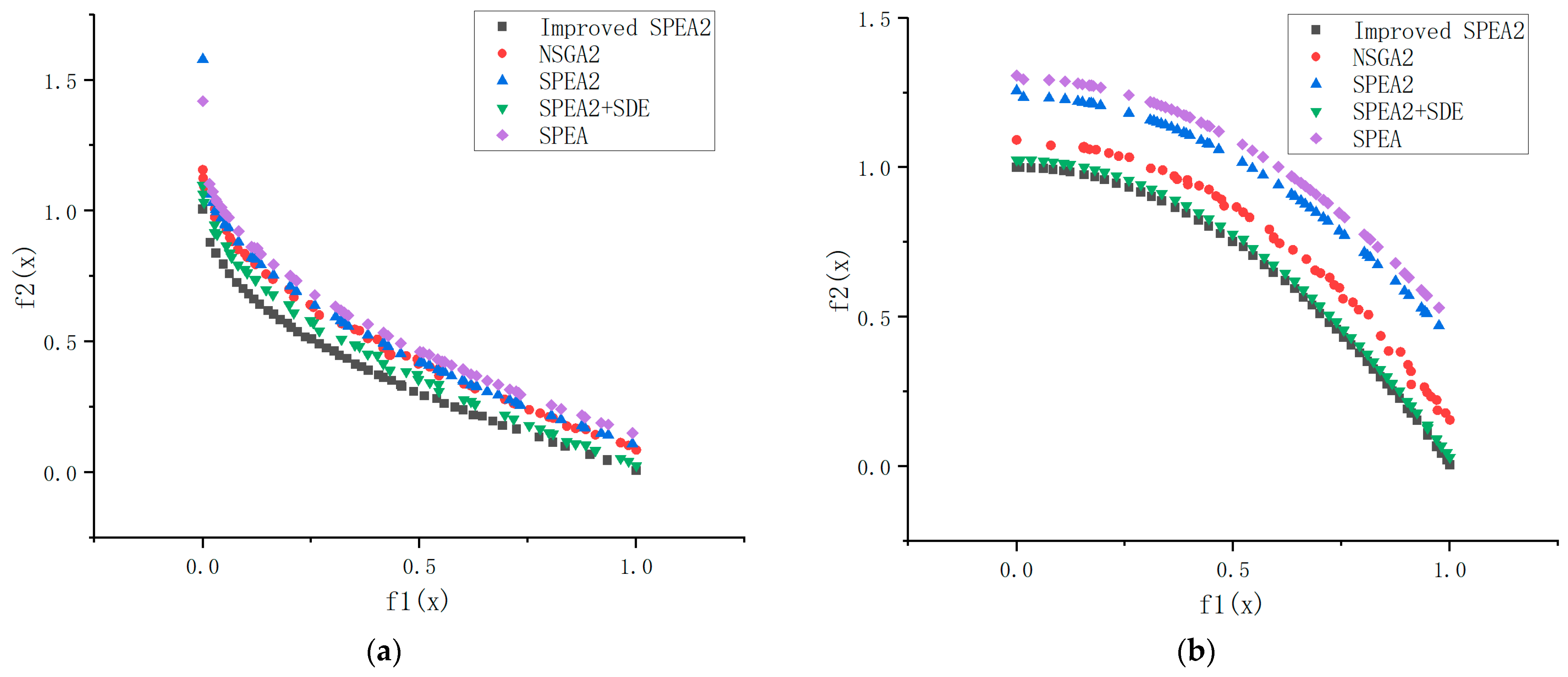
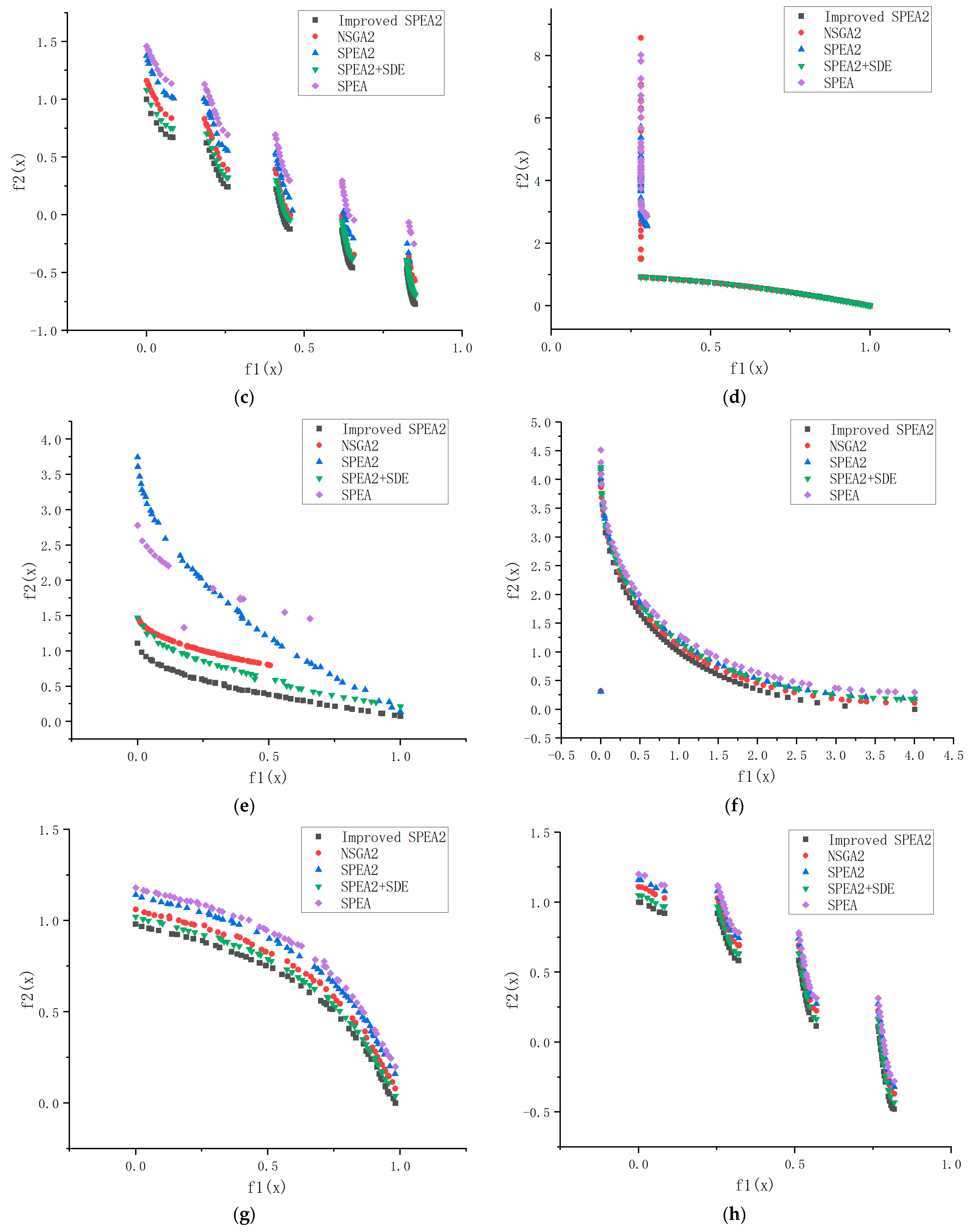
5.4. Simulation Experiment

In Section 5.2, the improved algorithm was tested on nine benchmark functions. From those experiments, we can see that the improved algorithm has certain advantages. In addition, we also wanted to verify whether the improved algorithm still achieved better results in the established UAV delivery model. Therefore, a certain number of distribution centers and delivery points were randomly generated in the city. We then compared the improved algorithm with the SPEA2, NSGA2, SPEA2 + SDE, and SPEA in the scene.
We set the crossover probability as 0.5, mutation probability as 0.5, population as 100, iteration times as 100, and test times as 20. Figure 8, below, shows the average results of the 20 experiments on these five algorithms, under the UAV delivery model in this paper.
Figure 9 shows the experimental results when the number of tasks is 30 and 100, respectively. The two factors that affect customer satisfaction are actually related to time. The goods decay over time, and late delivery will also have an impact. Therefore, the ‘Time cost’ on the vertical axis does not mean that time is a goal, but refers to the customer satisfaction. The abscissa is the other object, namely the ‘Distance cost’. From the perspective of the algorithm, the improved algorithm has better Pareto frontiers. It has better continuity, and is closer to the origin. This indicates that the improved algorithm is stable, and gives better results. On the other hand, from the perspective of the simulation, when the total distance of the UAVs is the same, the smaller the value of the improved SPEA2 in the vertical coordinate, the higher the customer satisfaction. When the customer satisfaction is the same, the path planned by the improved SPEA2 is shorter. This comparison is especially evident when the number of tasks is 100; for example, when the distance cost is 1, the customer satisfaction of the improved algorithm is more than 20% higher than that of other algorithms. That is to say, the improved algorithm always yields more benefits, regardless of the options chosen by the decision-maker.
To illustrate the comparison of the five algorithms, the generation distance proposed by Deb [18], and the spacing index proposed by Schott [67] are used in the quantitative analysis of the algorithms. The comparison results are shown in Figure 10 and Figure 11:
Their 95% confidence intervals are shown in Table 3:
Figure 10 and Figure 11 are box diagrams, drawn according to the values of the generational distance and spacing that were obtained by testing the objective function 20 times, and with the number of tasks as 30. All the box diagrams were drawn using Origin software. It can be seen that the values of the generation distance and spacing obtained by the improved SPEA2 are always less than those obtained by the SPEA2, NSGA2, SPEA2 + SDE, and SPEA. The average generational distance value of the improved algorithm is about 30% smaller than the second one, and the average spacing value is about 20% smaller. At the same time, the volatility of the improved SPEA2 is relatively low, which shows that it has advantages and stability in solving the problems of UAV delivery.

6. Conclusions

With the rise of the e-commerce industry, the UAV delivery of goods has gradually become more and more a delivery method that is discussed in daily life. It can reduce the dependence on manpower, reduce the transportation distance, and plan flexible routes. In addition, with the increasing demand for perishables, it has become an important issue to provide customers with goods as fresh as possible. There is no doubt that vehicles with a better refrigeration effect can be used for transportation; that is, keeping perishables fresh as much as possible during transportation. However, this paper aimed to improve the customer satisfaction without changing the transport vehicle, which required planning a more reasonable path. Therefore, a bi-objective model was established, with the distance cost and customer satisfaction as the objectives. Based on analysis of the model, the SPEA2 was adopted and improved. When improving the SPEA2, the idea of a local search was introduced, to determine the dominant and non-dominant solutions. In this way, on the basis of ensuring the excellent global search ability of the SPEA2, its poor local search ability was also strengthened. The improved algorithm not only maintains the diversity of the solution set, but also obtains results closer to the Pareto front. It shows a good performance, in theory and in experiments. Therefore, it has a high application value in UAV cargo delivery, and other MOPs.
(1)
The improved SPEA2, SPEA2, NSGA2, SPEA2 + SDE, and SPEA were tested through nine classical test functions. Compared with the other four algorithms, the convergence of the improved SPEA2, and the stability of the Pareto solution set are significantly improved.
(2)
In the empirical analysis, the improved SPEA2 is nearer to the theoretical Pareto front than the SPEA2, NSGA2, SPEA2 + SDE, and SPEA, and the result delivery is more uniform and stable. The convergence and stability of the algorithm were verified according to the aspects of the Pareto front, generational distance, and spacing. Through comprehensive analysis, the improved SPEA2 has been made more effective in dealing with the delivery of UAVs with hard time windows, and can achieve better results.
Although the improved SPEA2 can effectively solve the bi-objective UAV delivery problem, it failed to perform well on models with more objectives. We will further improve the multi-objective algorithm so that it can perform well when facing problems with more than five objectives. On the other hand, the effect of the traffic conditions on the problem is not taken into account in the model of this paper, because it involves a dynamic environment. In our follow-up work, we will try to incorporate the dynamic environment, to solve more complex problems.

Author Contributions

Conceptualization, Y.S.; methodology, Y.S.; software, Y.S.; validation, Y.S.; writing—original draft, Y.S.; conceptualization, X.F.; supervision, X.F.; writing—review and editing, X.F. All authors have read and agreed to the published version of the manuscript.

Funding

This work was supported by the Equipment Pre-Research Ministry of Education Joint Fund [grant number 6141A02033703].

Data Availability Statement

The data used to support the findings of this study are available from the corresponding author upon request.

Conflicts of Interest

The authors declare that they have no known competing financial interest or personal relationships that could have appeared to influence the work reported in this paper.

References

  1. Zhang, Z.; Zhang, Z.; Chen, X. Research on Location Selection of UAV Distribution Center Based on Improved Gravity Method. J. Phys. Conf. Ser. 2020, 1624, 052029. [Google Scholar] [CrossRef]
  2. Chopra, O.; Ghose, D. Distributed Control for Multiple UAV Transport of Slung Loads. In Proceedings of the AIAA Science and Technology Forum and Exposition, San Diego, CA, USA, 3–7 January 2022. [Google Scholar]
  3. Choi, T.-M. Innovative “Bring-Service-Near-Your-Home” operations under Corona-Virus (COVID-19/SARS-CoV-2) outbreak: Can logistics become the Messiah? Transp. Res. Part E Logist. Transp. Rev. 2020, 140, 101961. [Google Scholar] [CrossRef] [PubMed]
  4. Yang, Y.; Chi, H.; Zhou, W.; Fan, T.; Piramuthu, S. Deterioration control decision support for perishable inventory management. Decis. Support Syst. 2020, 134, 113308. [Google Scholar] [CrossRef]
  5. Zhang, Q.; Zheng, X.; Yang, S.; Li, C.; Wang, K. Evaluation and Cluster Analysis of E-Businesses with Perishable Products and Cold Supply Chain. In Proceedings of the 2018 15th International Conference on Service Systems and Service Management (ICSSSM), Hangzhou, China, 21–22 July 2018; IEEE: Piscataway Township, NJ, USA; pp. 1–6. [Google Scholar]
  6. Zitzler, E.; Deb, K.; Thiele, L. Comparison of multi-objective evolutionary algorithms: Empirical study. Evol. Comput. 2000, 8, 173–195. [Google Scholar] [CrossRef] [Green Version]
  7. Zhang, Q.; Zhang, J.; Zhong, Y.; Ye, C.; Min, X. Parallel MOEA Based on Consensus and Membrane Structure for Inferring Phylogenetic Reconstruction. IEEE Access 2019, 8, 6177–6189. [Google Scholar] [CrossRef]
  8. Chen, H.; Tian, Y.; Pedrycz, W.; Wu, G.; Wang, R.; Wang, L. Hyperplane Assisted Evolutionary Algorithm for Many-Objective Optimization Problems. IEEE Trans. Cybern. 2019, 7, 3367–3380. [Google Scholar] [CrossRef]
  9. Huang, W.; Zhang, Y.; Li, L. Survey on Multi-Objective Evolutionary Algorithms. J. Phys. Conf. Ser. 2019, 1288, 012057. [Google Scholar] [CrossRef]
  10. Yu, B.; Gu, T.; Chang, L.; Li, L.; Lan, R.; Sun, P. A Multi-Objective Evolutionary Algorithm Based on Adaptive Grid. In Proceedings of the 2019 9th International Conference on Information Science and Technology (ICIST), Hulunbuir, China, 2–5 August 2019; IEEE: Piscataway Township, NJ, USA, 2019. [Google Scholar]
  11. Schaffer, J.D. Multiple objective optimization with vector evaluated genetic algorithms. In Proceedings of the 1st International Conference on Genetic Algorithms, Broadway Hillsdale, NJ, USA, 1 July 1985; L. Erlbaum Associates Inc.: Mahwah, NJ, USA, 1985; pp. 93–100. [Google Scholar]
  12. Murata, T.; Ishibuchi, H. MOGA: Multi-objective genetic algorithms. In Proceedings of the 2nd IEEE International Conference on Evolutionary Computing, Perth, WA, Australia, 29 November–1 December 1995; Volume 2, pp. 289–294. [Google Scholar]
  13. Srinivas, N.; Deb, K. Multiobjective optimization using nondominated sorting in genetic algorithms. Evol. Comput. 1994, 2, 221–248. [Google Scholar] [CrossRef]
  14. Horn, J.; Nafpliotis, N.; Goldberg, D.E. A niched Pareto genetic algorithm for multiobjective optimization. In Proceedings of the First IEEE Conference on Evolutionary Computation, IEEE World Congress on Computational Intelligence, Orlando, FL, USA, 27–29 June 1994; IEEE Press: Piscataway, NJ, USA, 1994; Volume 1, pp. 82–87. [Google Scholar]
  15. Jiao, L.; Shang, R.; Liu, F.; Zhang, W. Theoretical basis of natural computation. In Brain and Nature-Inspired Learning Computation and Recognition; Elsevier: Amsterdam, The Netherlands, 2020; pp. 81–95. [Google Scholar]
  16. Zitzler, E.; Thiele, L. Multiobjective Evolutionary Algorithms: A Comparative Case Study and the Strength Pareto Evolutionary Algorithm. IEEE Trans. Evol. Comput. 1999, 3, 257–271. [Google Scholar] [CrossRef] [Green Version]
  17. Zitzler, E.; Laumanns, M.; Thiele, L. SPEA2: Improving the strength Pareto evolutionary algorithm. In Evolutionary Methods for Design, Optimization and Control with Applications to Industrial Problems; Springer: Berlin/Heidelberg, Germany, 2002; pp. 95–100. [Google Scholar]
  18. Deb, K.; Pratap, A.; Agarwal, S.; Meyarivan, T. A Fast and Elitist Multi-objective Genetic Algorithm: NSGA2. IEEE Trans. Evol. Comput. 2002, 6, 182–197. [Google Scholar] [CrossRef] [Green Version]
  19. Knowles, J.D.; Corne, D.W. Approximating the nondominated front using the Pareto archived evolution strategy. Evol. Comput. 2000, 8, 149–172. [Google Scholar] [CrossRef]
  20. Erickson, M.; Mayer, A.; Horn, J. The niched pareto genetic algorithm 2 applied to the design of groundwater remediation systems. In Evolutionary Multi-Criterion Optimization; Springer: Berlin/Heidelberg, Germany, 2001; pp. 681–695. [Google Scholar]
  21. Corne, D.W.; Knowles, J.D.; Oates, M.J. The Pareto envelope-based selection algorithm for multiobjective optimization. In Parallel Problem Solving from Nature PPSN VI; Springer: Berlin/Heidelberg, Germany, 2000; pp. 839–848. [Google Scholar]
  22. Corne, D.W.; Jerram, N.R.; Knowles, J.D.; Oates, M.J. PESA-II: Region-based selection in evolutionary multiobjective optimization. In Proceedings of the Genetic and Evolutionary Computation Conference (GECCO-2001), San Francisco, CA, USA, 7–11 July 2011; Morgan Kaufmann Publishers: Burlington, MA, USA, 2001; pp. 283–290. [Google Scholar]
  23. Zhou, A.; Qu, B.-Y.; Li, H.; Zhao, S.-Z.; Suganthan, P.N.; Zhang, Q. Multiobjective evolutionary algorithms: A survey of the state of the art. Swarm Evol. Comput. 2011, 1, 32–49. [Google Scholar] [CrossRef]
  24. Li, B.; Li, J.; Tang, K.; Yao, X. Many-objective evolutionary algorithms: A survey. ACM Comput. Surv. 2015, 48, 13. [Google Scholar] [CrossRef] [Green Version]
  25. Li, K.; Wang, R.; Zhang, T.; Ishibuchi, H. Evolutionary many-objective optimization: A comparative study of the state-of-the-art. IEEE Access 2018, 6, 26194–26214. [Google Scholar] [CrossRef]
  26. Huseyinov, I.; Bayrakdar, A. Performance Evaluation of NSGA-III and SPEA2 in Solving a Multi-Objective Single-Period Multi-Item Inventory Problem. In Proceedings of the 2019 4th International Conference on Computer Science and Engineering (UBMK), Samsun, Turkey, 11–15 September 2019. [Google Scholar]
  27. Moscato, P. On Evolution, Search, Optimization, Genetic Algorithms and Martial Arts: Towards Memetic Algorithms. Caltech Concurr. Comput. Program C3P Rep. 1989, 826, 37. [Google Scholar]
  28. Moscato, P.; Norman, M.G. A memetic approach for the traveling salesman problem implementation of a computational ecology for combinatorial optimization on message-passing systems. Parallel Comput. Transput. Appl. 1992, 1, 177–186. [Google Scholar]
  29. Dawkins, R. The Selfish Gene; Oxford University Press: Oxford, UK, 2016. [Google Scholar]
  30. Clodomir, S.; Marcos, O.; Carmelo, B.; Menezes, R. Beyond exploitation: Measuring the impact of local search in swarm-based memetic algorithms through the interactions of individuals in the population. Swarm Evol. Comput. 2022, 70, 101040. [Google Scholar]
  31. Mu, C.-H.; Xie, J.; Liu, Y.; Chen, F.; Liu, Y.; Jiao, L.-C. Memetic algorithm with simulated annealing strategy and tightness greedy optimization for community detection in networks. Appl. Soft Comput. 2015, 34, 485–501. [Google Scholar] [CrossRef]
  32. Acampora, G.; Cataudella, V.; Hegde, P.R.; Lucignano, P.; Passarelli, G.; Vitiello, A. Memetic algorithms for mapping p-body interacting systems in effective quantum 2-body Hamiltonians. Appl. Soft Comput. 2021, 110, 107634. [Google Scholar] [CrossRef]
  33. Vuppuluri, P.; Chellapilla, P. Serial and parallel memetic algorithms for the bounded diameter minimum spanning tree problem. Expert Syst. 2021, 38, e12610. [Google Scholar] [CrossRef]
  34. Nguyen, P.T.H.; Sudholt, D. Memetic algorithms outperform evolutionary algorithms in multimodal optimization. Artif. Intell. 2020, 287, 103345. [Google Scholar] [CrossRef]
  35. Tarantilis, C.D.; Kiranoudis, C.T. A meta-heuristic algorithm for the efficient distribution of perishable foods. J. Food Eng. 2001, 50, 1–9. [Google Scholar] [CrossRef]
  36. Rabbani, M.; Farshbaf-Geranmayeh, A.; Haghjoo, N. Vehicle routing problem with considering multi-middle depots for perishable food delivery. Uncertain Supply Chain. Manag. 2016, 4, 171–182. [Google Scholar] [CrossRef]
  37. Alvarez, A.; Cordeau, J.-F.; Jans, R.; Munari, P.; Morabito, R. Formulations, branch-and-cut and a hybrid heuristic algorithm for an inventory routing problem with perishable products. Eur. J. Oper. Res. 2020, 283, 511–529. [Google Scholar] [CrossRef]
  38. Liang, Y.; Liu, F.; Lim, A.; Zhang, D. An integrated route, temperature and humidity planning problem for the distribution of perishable products. Comput. Ind. Eng. 2020, 147, 106623. [Google Scholar] [CrossRef]
  39. Meneghetti, A.; Ceschia, S. Energy-efficient frozen food transports: The Refrigerated Routing Problem. Int. J. Prod. Res. 2020, 58, 4164–4181. [Google Scholar] [CrossRef]
  40. Wang, Y.; Li, Q.; Guan, X.; Xu, M.; Liu, Y.; Wang, H. Two-echelon collaborative multi-depot multi-period vehicle routing problem. Expert Syst. Appl. 2021, 114201, 167. [Google Scholar] [CrossRef]
  41. Tirkolaee, E.B.; Aydin, N.S. Integrated design of sustainable supply chain and transportation network using a fuzzy bi-level decision support system for perishable products. Expert Syst. Appl. 2022, 195, 116628. [Google Scholar] [CrossRef]
  42. Cardozo, R.N. An Experimental Study of Customer Effort, Expectation, and Satisfaction. J. Mark. Res. 1965, 2, 244. [Google Scholar] [CrossRef]
  43. Rahimi, M.; Baboli, A.; Rekik, Y. A bi-objective inventory routing problem by considering customer satisfaction level in context of perishable product. In Proceedings of the 2014 IEEE Symposium on Computational Intelligence in Production and Logistics Systems (CIPLS), Orlando, FL, USA, 9–12 December 2014; IEEE: Piscataway Township, NJ, USA, 2014; pp. 91–97. [Google Scholar]
  44. Wang, X.; Sun, X.; Dong, J.; Jie, D.; Meng, W. Optimizing Terminal Delivery of Perishable Products considering Customer Satisfaction. Math. Probl. Eng. 2017, 2017, 1–12. [Google Scholar] [CrossRef] [Green Version]
  45. Li, Y.; Chu, F.; Feng, C.; Chu, C.; Zhou, M. Integrated Production Inventory Routing Planning for Intelligent Food Logistics Systems. IEEE Trans. Intell. Transp. Syst. 2019, 20, 867–878. [Google Scholar] [CrossRef]
  46. Liang, X.; Wang, N.; Zhang, M.; Jiang, B. Bi-objective multi-period vehicle routing for perishable goods delivery considering customer satisfaction. Expert Syst. Appl. 2023, 220, 119712. [Google Scholar] [CrossRef]
  47. Labuza, T.P. Application of chemical kinetics to deterioration of foods. J. Chem. Educ. 1984, 61, 348. [Google Scholar] [CrossRef] [Green Version]
  48. Wang, X.; Li, D. A dynamic product quality evaluation-based pricing model for perishable food supply chains. Omega 2012, 40, 906–917. [Google Scholar] [CrossRef]
  49. Li, Y.; Yang, W.; Huang, B. Impact of UAV Delivery on Sustainability and Costs under Traffic Restrictions. Math. Probl. Eng. 2020, 2020, 9437605. [Google Scholar] [CrossRef]
  50. Zhou, B.; Huang, H.; Xu, Y.; Li, X.; Gao, H.; Chen, T.; Liu, X.; Xu, J. Parallel task scheduling algorithm based on collaborative device and edge in UAV delivery system. Jisuanji Jicheng Zhizao Xitong/Comput. Integr. Manuf. Syst. CIMS 2021, 27, 2575–2582. [Google Scholar]
  51. Cao, Z.; Wang, Z.; Zhao, L.; Fan, F.; Sun, Y. Multi-constraint and multi-objective optimization of free-form reticulated shells using improved optimization algorithm. Eng. Struct. 2022, 250, 113442. [Google Scholar] [CrossRef]
  52. Xue, Y.; Li, M.; Shepperd, M.; Lauria, S.; Liu, X. A novel aggregation-based dominance for Pareto-based evolutionary algorithms to configure software product lines. Neurocomputing 2019, 364, 32–48. [Google Scholar] [CrossRef]
  53. Coello, C.A.C.; Veldhuizen, D.A.V.; Lamont, G.B. Multi-Criteria Decision Making. In Genetic Algorithms and Evolutionary Computation Evolutionary Algorithms for Solving Multi-Objective Problems; Springer: Berlin/Heidelberg, Germany, 2002; pp. 321–347. [Google Scholar]
  54. Viguier, F.; Pierreval, H. An Approach to The Design of a Hybrid Organization of Workshops into Functional Layout and Group Technology Cells. Int. J. Comput. Integr. Manuf. 2004, 17, 108–116. [Google Scholar] [CrossRef]
  55. Zhao, H.; Zhang, C.; Zhang, B.; Duan, P.; Yang, Y. Decomposition-Based Sub-Problem Optimal Solution Updating Direction-Guided Evolutionary Many-Objective Algorithm. Inf. Sci. 2018, 448–449, 91–111. [Google Scholar] [CrossRef]
  56. Li, H.; Chen, F.; Ji, X.; Li, J.; Zhou, J. Master production plan of parallel casting workshop based on improved SPEA2. Jisuanji Jicheng Zhizao Xitong/Comput. Integr. Manuf. Syst. 2021, 27, 1072–1080. [Google Scholar]
  57. Duan, T.; Wang, W.; Li, X.; Wang, T.; Chen, X.; Zhou, X. Intelligent Collaborative Architecture Design based on Unmanned Combat Swarm. In Proceedings of the 2020 6th International Conference on Big Data and Information Analytics (BigDIA), Shenzhen, China, 4–6 December 2020. [Google Scholar]
  58. Lin, F.; Zeng, J.; Xiahou, J.; Wang, B.; Zeng, W.; Lv, H. Multi-Objective Evolutionary Algorithm Based on Non-Dominated Sorting and Bidirectional Local Search for Big Data. IEEE Trans. Ind. Inform. 2017, 13, 1979–1988. [Google Scholar] [CrossRef]
  59. Dariane, A.B.; Sabokdast, M.M.; Karami, F.; Asadi, R.; Ponnambalam, K.; Mousavi, S.J. Integrated operation of multi-reservoir and many-objective system using fuzzified hedging rule and strength pareto evolutionary optimization algorithm (SPEA2). Water 2021, 13, 1995. [Google Scholar] [CrossRef]
  60. Yu, W.; Zhang, L. Many-objective evolutionary computation based on adaptive hypersphere dynamic angle vector dominance. Concurr. Comput. Pract. Exp. 2021, 33, e6238. [Google Scholar] [CrossRef]
  61. Liu, X.; Zhang, D. An Improved SPEA2 Algorithm with Local Search for Multi-Objective Investment Decision-Making. Appl. Sci. 2019, 9, 1675. [Google Scholar] [CrossRef] [Green Version]
  62. Xia, M.; Zhang, C.; Weng, L.; Liu, J.; Wang, Y.; Tiwari, S.; Trivedi, M.; Kohle, M.L. Robot path planning based on multi-objective optimization with local search. J. Intell. Fuzzy Syst. 2018, 35, 1755–1764. [Google Scholar] [CrossRef]
  63. Tian, Y.; Cheng, R.; Zhang, X.; Jin, Y. PlatEMO: A MATLAB platform for evolutionary multi-objective optimization. IEEE Comput. Intell. Mag. 2017, 12, 73–87. [Google Scholar] [CrossRef] [Green Version]
  64. Liu, X.; Segura, S.; Zheng, W.; Segura, S.; Zheng, W. SIP: Optimal product selection from feature models using many Objective evolutionary optimization. ACM Trans. Softw. Eng. Methodol. 2016, 25, 1–39. [Google Scholar]
  65. Sayyad, A.S.; Ingram, J.; Menzies, T.; Ammar, H. Scalable product line configuration: A straw to break the camel’s back. In Proceedings of the 2013 28th IEEE/ACM International Conference on Automated Software Engineering (ASE), Silicon Valley, CA, USA, 11–15 November 2013; IEEE: Piscataway, NJ, USA, 2013. [Google Scholar]
  66. Fleischer, M. The Measure of Pareto Optima: Applications to Multi-objective Metaheuristics. In Proceedings of the International Conference on Evolutionary Multi-Criterion Optimization, Faro, Portugal, 8–11 April 2003; Springer: Berlin/Heidelberg, Germany, 2003; pp. 519–533. [Google Scholar]
  67. Schott, J.R. Fault Tolerant Design Using Single and Multicriteria Genetic Algorithm Optimization. Master’s Thesis, Department of Aeronautics and Astronautics, Massachusetts Institute of Technology, Cambridge, MA, USA, 1995. [Google Scholar]
Figure 1. The SPEA2 flow.
Mathematics 11 03327 g001
Figure 2. The fitness allocation method of the SPEA2.
Mathematics 11 03327 g002
Figure 3. The local search strategy.
Mathematics 11 03327 g003
Figure 4. The optimal solution sets of five algorithms under nine benchmark functions: (a) F 1 ; (b) F 2 ; (c) F 3 ; (d) F 4 ; (e) F 5 ; (f) F 6 ; (g) F 7 ; (h) F 8 ; and (i) F 9 .
Mathematics 11 03327 g004aMathematics 11 03327 g004bMathematics 11 03327 g004c
Figure 5. The convergence of the five algorithms under four benchmark functions: (a) F 1 ; (b) F 2 ; (c) F 3 ; and (d) F 4 .
Mathematics 11 03327 g005
Figure 6. The parameter experiments on F 1 : (a) mutation operator is 0.1; (b) mutation operator is 0.3; (c) mutation operator is 0.5; (d) mutation operator is 0.7; (e) mutation operator is 0.9; and (f) the best cases for different operations.
Mathematics 11 03327 g006
Figure 7. The parameter experiments on F 2 : (a) mutation operator is 0.1; (b) mutation operator is 0.3; (c) mutation operator is 0.5; (d) mutation operator is 0.7; (e) mutation operator is 0.9; and (f) the best cases for different operations.
Mathematics 11 03327 g007
Figure 8. The parameter experiments on F 3 : (a) mutation operator is 0.1; (b) mutation operator is 0.3; (c) mutation operator is 0.5; (d) mutation operator is 0.7; (e) mutation operator is 0.9; and (f) the best cases for different operations.
Mathematics 11 03327 g008
Figure 9. The results of the five algorithms: (a) number of tasks = 30; (b) number of tasks = 100.
Mathematics 11 03327 g009
Figure 10. The generational distance values.
Mathematics 11 03327 g010
Figure 11. The spacing values.
Mathematics 11 03327 g011
Table 1. The benchmark functions.
FunctionDimRange
F 1 M i n   F 1 x = f 1 x , f 2 x
f 1 x = x f 2 x = g 1 f 1 / g
g x = 1 + 9 i = 2 m x i / m 1
30[0, 1]
F 2 M i n   F 2 x = f 1 x , f 2 x
f 1 x = x f 2 x = g 1 f 1 / g 2
g x = 1 + 9 i = 2 m x i / m 1
30[0, 1]
F 3 M i n   F 3 x = f 1 x , f 2 x
f 1 x = x f 2 x = g 1 f 1 g f 1 / g s i n 10 π f 1
g x = 1 + 9 i = 2 m x i / m 1
30[0, 1]
F 4 M i n   F 4 x = f 1 x , f 2 x
f 1 x = 1 e 4 x s i n 6 6 π x f 2 x = g 1 f 1 / g 2
g x = 1 + 9 i = 2 m x i m 1 0.25
30[0, 1]
F 5 M i n   F 5 x = f 1 x , f 2 x
f 1 x = x f 2 x = g 1 f 1 / g
g x = 1 + 10 m 1 + i = 2 m x i 2 10 cos 4 π x i
10[−5, 5]
F 6 M i n   F 6 x = f 1 x , f 2 x
f 1 x = x 2 f 2 x = x 2 2
100 [ 10 5 ,     10 5 ]
F 7 M i n   F 7 x = f 1 x , f 2 x
f 1 x = 1 e i = 1 3 x i 1 3 ^ 2 f 2 x = 1 e i = 1 3 x i + 1 3 ^ 2
3[−4, 4]
F 8 M i n   F 8 x = f 1 x , f 2 x
f 1 x = x 1 f 2 x = 1 + 10 x 2 1 x 1 1 + 10 x 2 2 x 1 1 + 10 x 2 s i n 8 π x 1
20[0, 1]
F 9 M i n   F 9 x = f 1 x , f 2 x
f 1 x = i = 1 m 1 10 e 0.2 x i 2 + x i + 1 2 f 2 x = i = 1 m x i 0.8 + 5 s i n x i 3
3[−5, 5]
Table 2. The VN, TT100% and HV of five algorithms under nine test functions.
FunctionsIndexImproved SPEA2NSGA2SPEA2SPEA2 + SDESPEA
F 1 VN (20)2020202020
TT100%1.01.17.30.810.5
HV0.89340.87180.84390.87920.7957
F 2 VN (20)2020202020
TT100%1.51.69.71.214.4
HV0.88590.87310.83920.89170.8038
F 3 VN (20)2020202020
TT100%1.91.815.61.921.4
HV0.81260.79330.72790.80180.6817
F 4 VN (20)2020202020
TT100%2.62.724.82.435.7
HV0.85960.71510.61390.86380.5884
F 5 VN (20)2020182012
TT100%21.926.496.120.3183.7
HV0.83940.70620.60280.80450.4119
F 6 VN (20)2020202020
TT100%7.98.341.98.267.5
HV0.87830.85260.83130.86170.8106
F 7 VN (20)2020202020
TT100%25.728.5136.224.3207.3
HV0.79080.73470.72140.77050.7008
F 8 VN (20)2020202020
TT100%3.02.817.12.437.6
HV0.87690.85730.84910.87070.8327
F 9 VN (20)2020202020
TT100%11.913.250.410.6118.1
HV0.78390.76540.74860.77920.7218
Table 3. The 95% confidence intervals for the generational distance values and spacing values of the five algorithms.
IndexImproved SPEA2NSGA2SPEA2SPEA2 + SDESPEA
Generational distance[1.34 × 10⁻³, 2.60 × 10⁻³][2.34 × 10⁻³, 5.43 × 10⁻³][1.09 × 10⁻², 1.56 × 10⁻²][1.81 × 10⁻³, 3.48 × 10⁻³][1.43 × 10⁻², 1.92 × 10⁻²]
Spacing[8.55 × 10⁻⁴, 1.93 × 10⁻³][2.00 × 10⁻³, 3.97 × 10⁻³][3.27 × 10⁻³, 5.10 × 10⁻³][1.34 × 10⁻³, 2.60 × 10⁻³][4.40 × 10⁻³, 6.31 × 10⁻³]
Disclaimer/Publisher’s Note: The statements, opinions and data contained in all publications are solely those of the individual author(s) and contributor(s) and not of MDPI and/or the editor(s). MDPI and/or the editor(s) disclaim responsibility for any injury to people or property resulting from any ideas, methods, instructions or products referred to in the content.

