Article

Hypergraph-Regularized Lp Smooth Nonnegative Matrix Factorization for Data Representation

1
School of Mathematical Sciences, Guizhou Normal University, Guiyang 550025, China
2
School of Science, Kaili University, Kaili 556011, China
3
School of Mathematical Sciences, Xiamen University, Xiamen 361005, China
*
Author to whom correspondence should be addressed.
Mathematics 2023, 11(13), 2821; https://doi.org/10.3390/math11132821
Submission received: 17 May 2023 / Revised: 18 June 2023 / Accepted: 21 June 2023 / Published: 23 June 2023

Abstract

:
Nonnegative matrix factorization (NMF) has been shown to be a strong data representation technique, with applications in text mining, pattern recognition, image processing, clustering and other fields. In this paper, we propose a hypergraph-regularized L p smooth nonnegative matrix factorization (HGSNMF) by incorporating the hypergraph regularization term and the L p smoothing constraint term into the standard NMF model. The hypergraph regularization term can capture the intrinsic geometry structure of high dimension space data more comprehensively than simple graphs, and the L p smoothing constraint term may yield a smooth and more accurate solution to the optimization problem. The updating rules are given using multiplicative update techniques, and the convergence of the proposed method is theoretically investigated. The experimental results on five different data sets show that the proposed method has a better clustering effect than the related state-of-the-art methods in the vast majority of cases.

1. Introduction

Data representation plays an important role in information retrieval [1], computer vision [2], pattern recognition [3], and other applied fields [4,5]. There are many approaches to deal with high-dimensional data, such as data dimensionality reduction, random forests (RF) [6], multilayer perceptrons (MPL) [7], graph neural networks (GNN) [8], and hypergraph neural networks (HGNN) [9]. The dimensions of data matrices are extremely high in these practical applications. The high-dimensional data can not only cause storage difficulties, but also possible dimensional curses. Therefore, it is necessary to find an effective and low-dimensional representation of the original high-dimensional data matrix. It is also important to preserve the multidimensional structure of the image data and to preserve the multidimensional structure of the image data. Matrix factorization is one of the important data representation techniques, and typical matrix decomposition methods mainly include the following: principal component analysis (PCA) [10], linear discriminant analysis (LDA) [11], singular value decomposition (SVD) [12], nonnegative matrix factorization (NMF) [13,14], and so on. The tensor of a multidimensional array is well suited to representing such an image space, and, in order to extract valuable information from a given large tensor, a low-rank Tucker decomposition (TD) [15] is usually considered. In the real world, many data images, video volumes, and test data are non-negative, and, for these types of data, nonnegative Tucker decomposition (NTD) has recently received attention [16,17,18,19].
NMF has been gaining popularity through the works of Lee and Seung that were published in Nature [13] and NIPS [14]. It has been widely applied in clustering [20,21,22], face recognition [23,24], text mining [25,26], image processing [27,28,29], hyperspectral unmixing (HU) [30,31], and other fields [32,33,34,35]. Several NMF versions have been presented in order to improve data representation capabilities by introducing different regularization terms or constraint terms into the basis NMF model. For example, by considering the orthogonality of factor matrices, Ding et al. [21] presented a orthogonal nonnegative matrix tri-factorization (ONMF) approach. By incorporating the graph regularization term into the standard NMF model, Cai et al. [2] presented a graph-regularized nonnegative matrix factorization (GNMF) method, where a simple nearest neighborhood graph is constructed by considering the pairwise geometric relationships between two sample points. However, the model did not take into account the high-order relationships among multiple sample points. Shang et al. [36] presented a graph dual regularization nonnegative matrix factorization (DNMF) approach, which simultaneously considers the intrinsic geometry matrix structures of both the data manifold and the feature manifold. However, their DNMF approach neglects the high-order relationships among multiple sample points or multiple features. To solve the above problem, Zeng et al. [37] presented the hypergraph-regularized nonnegative matrix factorization (HNMF) method, which incorporates the hypergraph regularization term into NMF and constructs a hypergraph by considering high-order relationships among multiple sample points. However, HNMF is unable to produce a smooth and precise solution, because it does not take into account the smoothness of the basis matrix. Recently, Leng et al. [38] proposed the graph-regularized L p smooth nonnegative matrix factorization (GSNMF) method by incorporating the graph regularization term and the L p smoothing term into the basis NMF model, which considers the intrinsic geometric structures of the sample data and may produce a smooth and more accurate solution to the optimization problem with the addition of the graph regularization term and the L p smoothing constraint. However, in GSNMF, only the pairwise relationships between two sample points are considered, and the high-order relationships among multiple sample points are ignored.
Base on NTD, Qiu et al. [39] proposed a graph-regularized non-negative Tucker decomposition (GNTD) method, which is able to extract a representation based on low-dimensional parts from high-dimensional tensor data and retain geometric information. Immediately after, Qiu et al. [40] gave an alternating approximate gradient descent method to solve the proposed GNTD framework (UGNTD).

1.1. Problem Statement

In this paper, by incorporating hypergraph regularization and L p smoothing constraint terms into the standard NMF model, we propose a hypergraph-regularized L p smooth nonnegative matrix factorization (HGSNMF) method. The hypergraph regularization term considers the high-order relationships among multiple samples. The L p smoothing constraint term takes into account the smoothness of the basis matrix, which has been proven to be significant in data representation [41,42,43]. To solve the optimization problem of the HGSNMF model, we offer an effective optimization algorithm using the multiplicative update technique and theoretically prove the convergence of the HGSNMF algorithm. Finally, we conducted comprehensive experiments on five data sets to demonstrate the effectiveness of the proposed method.

1.2. Research Contribution

The main contributions of this work can be summarized as follows:
(1) Considering the complex relationships as pairwise relationships in a simple graph will inevitably lead to loss of the important information. Therefore, we construct the hypergraph regularization term to better discover the hidden semantics and simultaneously capture the underlying intrinsic geometric structure of high-dimensional spatial data samples. When constructing a hypergraph, each vertex of the hypergraph represents a data sample, and each vertex forms a hyperedge with its k nearest neighboring samples. Each hyperedge represents the similarity relationship between a group of samples with higher similarity.
(2) We consider the L p smoothing constraint of the basis matrix, which not only removes the noise of the basis matrix to make it smooth, but also obtains a smooth and more accurate solution to the optimization problem by combining the advantages of isotropic and diffusion anisotropic smoothing.
(3) We solve the optimization problem using an efficient iterative technique and conducted comprehensive experiments to empirically analyze our approach on five data sets; the experimental results validate the effectiveness of our proposed method.
The rest of the paper is organized as follows. In Section 2, we introduce some related works, including NMF, GSNMF, and hypergraph learning. In Section 3, we propose the novel HGSNMF model in detail, as well as its updating rules, and prove the convergence of the HGSNMF method. We also analyse the complexity of the proposed method. In Section 4, we provide the results extensive experiments that were conducted to validate the proposed method. Finally, we conclude this paper in Section 5.

2. Related Work

2.1. Nonnegative Matrix Factorization

Given a nonnegative matrix  X = [ x 1 , x 2 , , x n ] R + m × n , each column x i R + m ( i = 1 , 2 , , n ) of X represents a data point. The purpose of NMF is to decompose a nonnegative matrix into two low-rank nonnegative factor matrices B R + m × r and C R + r × n , whose product is an approximation of the original matrix. In particular, the objective function of NMF is
min X BC F 2 , s . t . B 0 , C 0 ,
where · F is the Frobenius norm of a matrix, B is the basis matrix, and C is the coefficient matrix (also called the encoding matrix). Obviously, the objective function is convex for B or C , but nonconvex for both B and C . Lee et al. [14] proposed the iterative multiplicative updating technique to solve the problem (1) as follows:
B i k B i k ( XC ) i k ( BCC ) i k , C k j C k j ( B X ) k j ( B BC ) k j ,
where B is the transpose of B .

2.2. Graph Regularization L p Smooth Nonnegative Matrix Factorization

GSNMF takes full account of the similarity between pairs of data points and the smoothness of the basis matrix, so it adds the graph regularity term and the L p smoothness term into the basis NMF model. Specifically, the objective function of GSNMF is
min X BC F 2 + α Tr ( C L C ) + 2 μ | | B | | p p , s . t . B 0 , C 0 ,
where Tr ( · ) denotes the trace of a matrix, α > 0 , μ > 0 , 1 < p 2 , L = D W is called as the graph Laplacian, and D is a diagonal matrix with D i i = Σ j W i j . W is the weight matrix whose value is given by [2]
W i j = x j e i exp ( | | x i x j | | 2 δ 2 ) , x i N k ( x j ) o r x j N k ( x i ) 0 , o t h e r w i s e
Leng et al. [38] used the iterative multiplicative updating technique to solve problem (2) as follows:
B i k B i k ( XC ) i k ( BCC ) i k + μ p B i k p 1 , C k j C k j ( B X ) k j + α ( CW ) k j ( B BC ) k j + α ( CD ) k j .

2.3. Hypergraph Learning

The simple graph only considers the pairwise geometric relationship between data samples; the complex internal structure of the data samples could not be used efficiently. To remedy this defect, the hypergraph takes into account the high-order geometric relationships among multiple samples, which can better capture the potential geometric information of the data [30]. Thus, hypergraph learning [44,45,46,47,48,49] is an extension of simple graph learning theory.
The hypergraph G = ( V , E ) takes into account the high-order relationships among multiple vertices and consists of a non-empty vertex set V = { v 1 , v 2 , , v n } and a non-empty hypergraph set E = { e 1 , e 2 , , e m } . Each element v i V is called a vertex, and each element e j E is a subset of V, which is known as a hyperedge of G. G is a hypergraph defined on V if e j for j = 1 , 2 , , m and e 1 e 2 e m = V .
When constructing a hypergraph, we generate the hyperedge by calculating the Euclidean distance between the k nearest neighbors (kNN) of each vertex. The parameter k is manually set. The kNN method allows the following steps to select k sample data points to construct the hypergraph. First, it calculates the distance between the sample data and the individual sample data. Then, it sorts according to the increasing relationship of the distances. Finally, it selects the k sample data points with the smallest distance. Obviously, kNN has the advantages of being simple, easy to understand, and easy to implement. Thus, we use kNN to construct the hypergraph. An incidence matrix H R + | V | × | E | is used to describe the incidence relationship between a vertex and a hyperedge, which is formalized as H ( v , e ) = 1 if v e and as H ( v , e ) = 0 otherwise.
Figure 1 gives an illustration of the simple graph, the hypergraph G ¯ = ( V ¯ , E ¯ ) , and an incidence matrix. If a vertex is in the k nearest neighbors of another vertex in the undirected simple graph, the two vertices are connected by an edge. The hypergraph G ¯ = ( V ¯ , E ¯ ) considers the high-order relationships among multiple vertices and is made up of a non-empty vertex set V ¯ = { v 1 , v 2 , v 3 , v 4 , v 5 , v 6 , v 7 , v 8 } and a non-empty hypergraph set E ¯ = { e 1 = { v 1 , v 2 , v 4 } , e 2 = { v 3 , v 4 , v 5 , v 6 } , e 3 = { v 6 , v 7 , v 8 } } . In Figure 1, the solid nodes stand for the vertices, while the node sets denoted by the solid line segment and the ellipses represent the hyperedges. Furthermore, each vertex in the hypergraph is connected to at least one hypheredge, which is associated with a weight, and each hyperedge can have multiple vertices.
Each hyperedge e can be assigned with a positive integer ω ( e ) that represents the weight of the hyperedge. The degree of a vertex v and the degree of a hyperedge can be expressed as d ( v ) = e E ω ( e ) H ( v , e ) and δ ( e ) = v V H ( v , e ) , respectively. According to [44], the unnormalized hypergraph Laplacian matrix can be expressed as
L H y p e r = D v S ,
where S = HWD e 1 H , H is an incidence matrix, W is a diagonal weight matrix composed of ω ( e ) , and D v and D e denote the diagonal matrices composed of d ( v ) and δ ( e ) , respectively.
There is a wide range for hypergraphs in computer vision, including classification and retrieval tasks. Feng et al. [9] put up the idea of a hypergraph neural network framework (HGNN) for learning data representation. Links are used in social networks. Chen et al. [50] made a methodical and thorough forecast regarding links. Yin et al. [51] presentend a hypergraph-regularized nonnegative tensor factorization for dimensionality reduction. In addition, Wang et al. [30] presented a hypergraph-regularized sparse NMF (HGLNMF) for hyperspectral unmixing, which incorporates the sparse term into HNMF. HGLNMF takes the sparsity of the coefficient matrix into account, and the hypergraph can simulate the higher-order relationship between multiple pixels by using multiple vertices in its hyperedges. Wu et al. [52] presented nonnegative matrix factorization with mixed hypergraph regularization (MHGNMF), by taking into account the higher-order information between the vertices. Some scholars apply nonnegative matrix factorization to multiple perspectives, Zhang et al. [53] presented semi-supervised multi-view clustering with dual-hypergraph-regularized partially shared nonnegative matrix factorization (DHPS-NMF). Huang et al. [54] presented diverse deep matrix factorization with hypergraph regularization for multiview data representation. To some extent, these approaches focus more on the multiple vertices hypergraph, which reflects the higher-order relationships between the multiple vertices, but they ignore the base matrix or its smoothness. To overcome this deficiency, we suggest the following hypergraph-regularized L p smooth nonnegative matrix factorization, which takes into account the higher-order relationships of numerous vertices, as well as the smoothness of the basis matrix.

3. Hypergraph-Regularized L p Smooth Nonnegative Matrix Factorization

In this section, we will describe the proposed HGSNMF approach in detail, as well as the iterative updating rules of two factor matrices. Then, the convergence of the proposed iterative updating rules is proven. Finally, the cost of calculating this approach is shown.
First, we give the construction of the hypergraph regularization term. Given a nonnegative data matrix X = [ x 1 , x 2 , , x n ] R + m × n , we expect that, if two data samples x i and x j are close, the corresponding encoding vectors c i and c j in the low-dimensional space are also close to each other. We encode geometrical information in the coefficient matrix hypergraph by linking each data sample with its k nearest neighbors and denoting their hypergraph connections with heat kernel weight:
ω ( e i ) = x j e i exp ( | | x i x j | | 2 δ 2 ) ,
where δ = 1 k n i = 1 n x j e i | | x i x j | | denotes the average distance among all the vertices.
With the weight ω ( e ) matrix defined above, the hypergraph regularization of the matrix C can be caculated by the following optimization problem:
R = 1 2 e E i , j e ω ( e ) δ ( e ) | | c i c j | | 2 = Tr C ( D v S ) C = Tr ( CL H y p e r C ) ,
where L H y p e r is the hypergraph Laplacian matrix of the hyergraph G and is defined by (3).

3.1. The Objective Function

To discover the intrinsic geometric structure information of a data set and produce a smooth and more accurate solution, we propose the HGSNMF method by incorporating hypergraph regularization and the L p smoothing constraint into NMF. The objective function of our HGSNMF is defined as follows:
min O = min B , C | | X BC | | F 2 + α Tr ( C L H y p e r C ) + 2 μ | | B | | p p , s . t . B 0 , C 0 ,
where B is the basis matrix, | | B | | p = i = 1 , j = 1 m , r ( B i j ) p 1 p , 0 < p 2 and p 1 , B i j is the ith row and jth column entry of matrix B , C is the coefficient matrix, and α and μ are the positive regularization parameters for balancing the reconstruction error in (5). The hypergraph regularization term and L p smoothing regularization term are presented in the second and the third terms, respectively. The hypergraph regularization term can more effectively discover the hidden semantics and simultaneously capture the underlying intrinsic geometric structure of the high-dimensional space data. The L p smoothing constraint of the basis matrix not only smooths the basis matrix by removing noise, but it also produces a smooth and more accurate solution to the optimization problem by combining the advantages of isotropic and diffusion anisotropic smoothing. Then, we give the detailed derivation of the updating rules, the theoretical proof of convergence, and an analysis of the computing complexity of the HGSNMF approach, as well as further comparative experiments.

3.2. Optimization Method

The objective function O in (5) is not convex in both B and C , so it is unrealistic to find the global optimal solution. Thus, we can only obtain the local optimal solution by using the iterative method. There are the multiplicative update, projective gradient, alternating direction multiplier, and dictionary learning algorithm for solving optimization problems. Because the multiplicative update algorithm has the advantages of convergence, simple operation, and small computation, we use the multiplicative update algorithm to solve optimization problems. We can turn the objective function into the following unconstrained objective function by using the Lagrange multiplier:
L = | | X BC | | F 2 + α Tr ( C L H y p e r C ) + 2 μ | | B | | p Tr ( Υ B ) Tr ( Λ C ) ,
where Υ = [ Υ i k ] , Λ = [ Λ k j ] , and Υ i k and Λ k j are the Lagrange multipliers for the constrains B i k 0 and C k j 0 , respectively.
By taking the partial derivatives of L with respect to B and C , respectively, we have that
L B = 2 BCC 2 XC + 2 μ p B p 1 Υ ,
L C = 2 B BC 2 B X + 2 α C L H y p e r Λ .
By using the Karush–Kuhn–Tucker (KKT) conditions L B = 0 , L C = 0 , Υ i k · B i k = 0 , and Λ k j · C k j = 0 , we obtain that
( BCC ) i k B i k + μ p B i k p 1 B i k ( XC ) i k B i k = 0 ,
( B BC ) k j C k j + α ( C L H y p e r ) k j C k j ( B X ) k j C k j = 0 .
According to (6) and (7), we can obtain the following updating rules for B and C :
B i k B i k ( XC ) i k ( BCC ) i k + μ p B i k p 1
and
C k j C k j ( B X ) k j + α ( CS ) k j ( B BC ) k j + α ( C D v ) k j ,
respectively.

3.3. Convergence Analysis

In this part, we demonstrate the convergence of our proposed HGSNMF in (5) by utilizing the updating rules (8) and (9). First of all, we introduce some related definitions and lemmas.
Definition 1 
([14]). G ( x , x ) is an auxiliary function of F ( x ) if G ( x , x ) satisfies the condition
G ( x , x ) F ( x ) , G ( x , x ) = F ( x ) .
The auxiliary function plays an important role due to the following lemma.
Lemma 1 
([14]). If G is an auxiliary function of F, then F is nonincreasing under the updating rule
x t + 1 = arg min x G ( x , x t ) .
To prove the convergence of HGSNMF under the updating step for B in (8), we fix the matrix C . For any element B i k in B , we use F ˜ i k to denote the part of the objective function O that is relevant only to B i k . The first and second derivatives of F ˜ ( B i k ) are given as follows:
F ˜ i k = O B i k = 2 ( BCC XC ) i k + 2 μ p ( B i k ) p 1
and
F ˜ i k = 2 O B 2 i k = 2 ( CC ) k k + 2 μ p ( p 1 ) ( B i k ) p 2 ,
respectively.
Lemma 2.
The function
G ˜ ( x , B i k t ) = F ˜ ( B i k t ) + F ˜ ( B i k t ) ( x B i k t ) + ( BCC ) i k + μ p ( B i k t ) p 1 B i k t ( x B i k t ) 2
is an auxiliary function of F ˜ i k ( x ) , which is only relevant to B i k .
Proof. 
From Taylor series expansion, we have that
F ˜ i k ( x ) = F ˜ ( B i k t ) + F ˜ ( B i k t ) ( x B i k t ) + ( CC ) k k ( x B i k t ) 2 + μ p ( p 1 ) ( B i k t ) p 2 ) ( x B i k t ) 2 .
Clearly, G ˜ ( x , x ) = F ˜ i k ( x ) . By Definition 1, we just need to prove that G ˜ ( x , B i k t ) F ˜ i k ( x ) . By comparing (11) with (12), we can find that G ˜ ( x , B i k t ) F ˜ i k ( x ) is equivalent to
( B CC ) i k + μ p ( B i k t ) p 1 B i k t ( CC ) k k + μ p ( p 1 ) ( B i k t ) p 2 .
B 0 , C 0 , 0 < p 2 , and p 1 , we have
( B CC ) i k = l = 1 , l k r B i l t ( CC ) l k + B i k t ( CC ) k k B i k t ( CC ) k k
and
p ( B i k t ) p 1 p ( p 1 ) ( B i k t ) p 1 .
Thus, (13) holds, which implies that G ˜ ( x , B i k t ) F ˜ i k ( x ) . □
Theorem 1.
The objective function O in (5) is nonincreasing under the updating rule of (8).
Proof. 
By replacing G ( x , x t ) in (10) with (11), we can obtain the updating rule
B i k t + 1 = B i k t B i k t F ˜ ( B i k t ) 2 ( B CC ) i k + 2 μ p ( B i k t ) p 1 = B i k t ( XC ) i k ( B CC ) i k + μ p ( B i k t ) p 1 .
Since (11) is an auxiliary function of F ˜ i k , F ˜ i k is nonincreasing under the updating rule of (8). □
Next, we fix the matrix B . For any element C k j in C , we use F ¯ k j to denote the part of the objective function O that is relevant only to C k j . By calculation,
F ¯ k j = O C k j = 2 ( B BC B X + α CL H y p e r ) k j
and
F ¯ k j = 2 O C 2 k j = 2 ( B B ) k k + 2 α ( L H y p e r ) j j .
Lemma 3.
The function
G ¯ ( x , C k j t ) = F ¯ ( C k j t ) + F ¯ ( C k j t ) ( x C k j t ) + ( B T BC + α C D v ) k j C k j t ( x C k j t ) 2
is an auxiliary function of F ¯ k j ( x ) , which is only relevant to C k j .
Proof. 
From Taylor series expansion, we have that
F ¯ k j ( x ) = F ¯ ( C k j t ) + F ¯ ( C k j t ) ( x C k j t ) + ( B B ) k k + α ( L H y p e r ) j j ) x C k j t ) 2 .
Clearly, G ¯ ( x , x ) = F ¯ k j ( x ) . According to Definition 1, we only need to prove that G ¯ ( x , C k j t ) F ¯ k j ( x ) . By comparing (15) with (16), we see that G ¯ ( x , C k j t ) F ¯ k j ( x ) is equivalent to
( B BC + α C D v ) k j C k j t ( B B ) k k + α ( L H y p e r ) j j .
Since B 0 and C 0 , we have
( B BC ) k j = l = 1 , l j n C k l t ( B B ) k k + C k j t ( B B ) k k C k j t ( B B ) k k
and
( C D v ) k j = l = 1 , l j n C k l t ( D v ) l j + C k j t ( D v ) j j C k j t ( D v S ) j j = C k j t ( L H y p e r ) j j .
Thus, (17) holds, which implies that G ¯ ( x , C k j t ) F ¯ k j ( x ) . □
Theorem 2.
The objective function O in (5) is nonincreasing under the updating rule of (9).
Proof. 
By replacing G ( x , x t ) in (10) with (15), we can obtain the updating rule:
C k j t + 1 = C k j t C k j t F ¯ ( C k j t ) 2 ( B BC + α C D v ) k j = C k j t ( B X + α C B ) k j ( B BC + α C D v ) k j .
Since (15) is an auxiliary function of F ¯ k j , F ¯ k j is nonincreasing under the updating rule of (9). □
Similar to NMF, it is known from Theorems 1 and 2 that the convergence of the model (5) can be guaranteed under the updating rules of (8) and (9).
The specific procedure for finding the local optimal B and C of HGSNMF is summarized in Algorithm 1.
For the specific implementation of Algorithm 1, we first repeat HGSNMF 10 times on the original data, and then this low-dimensional reduced data repeats K-means clustering 10 times.
Algorithm 1 HGSNMF algorithm.
Input: Data matrix X = [ x 1 , x 2 , , x n ] R + m × n . The number of neighbors k. The algorithm
parameters r, p and regularization parameters α , μ . The stopping criterion ϵ , and the maximum
number of iterations maxiter. Let Δ 0 = 1 e 5 .
Output: Factors B and C ;
1: Initialize B and C ;
2: Construct the weight matrix W using (4), and calculate the
   matrix D v , S ;
3: for  t = 1 , 2 , ,  maxiter do
4:    Update B t and Update C t according to (8), (9), respectively.
5:    Compute the objective function value O of (5) to denote Δ t .
6:    if  | Δ t Δ t 1 | Δ t 1 < ϵ ,
         Break and return  B , C .
7:    end if
8: end for

3.4. Computational Complexity Analysis

In this section, we analyze the computational complexity of the proposed HGSNMF method compared to other nonnegative matrix methods. The fladd, flmlt, and fldiv denote floating point addition, multiplication, and division, respectively. The O notation denotes the computational cost. The parameters n, m, r, and k denote the number of sample points, features, factors, and nearest neighbors to construct an edge or hyperedge, respectively.
According to the updating rules, we calculate the arithmetic operations of each iteration in HGSNMF and summarise the results of the proposed HGSNMF. From Table 1, we can see that the total cost of our proposed HGSNMF is O ( m n r ) .

4. Numerical Experimentation

In this section, we compare the results of data clustering on five popular data sets to estimate the performance of the proposed HGSNMF method with the related state-of-the-art methods, such as K-means, NMF [13], GNMF [2], HNMF [37], GSNMF [38], HGLNMF [30], GNTD [39], and UGNTD [40]. All tests were performed on a computer with a 2-Ghz Intel(R) Core(TM) i5-2500U CPU and 8-GB memory 64-bit using MATLAB R2015a in Windows 10. The stopping criterion was ϵ = 10 5 , and the maximum number of iterations was set to 10 4 .

4.1. Data Sets

The clustering performance was evaluated on five widely used data sets, including COIL20 (https://www.cs.columbia.edu/CAVE/software/softlib/coil-20.php (accessed on 26 October 2021)), YALE, Mnist, ORL (https://www.cad.zju.edu.cn/home/dengcai.Data/data.html, accessed on: 26 October 2021), and Georgia ((https://www.anefian.com/research/face-reco.htm (accessed on 26 October 2021)). The important statistical information of the five data sets is listed in Table 2, with more details given as follows.
(1) COIL20: The data set contains 72 grey-scale images for each of 20 objects viewed at varying angles.They were resized to 32 × 32 .
(2) ORL: The data set contains 10 different images of each of 40 human subjects. For some subjects, the images were taken at different times and different light conditions. They capture different facial expressions and different facial details. We resized them to 32 × 32 .
(3) YALE: The data set contains 11 grey-scale images for each of 15 individuals viewed at different facial expressions or configurations. These images were resized to 32 × 32 .
(4) Georgia: The data set contains 15 color JPEG grey face images for each of 50 people, with cluttered backgrounds for each object. We also resized them to 32 × 32 .
(5) Mnist: The data set contains 700 grey images of handwritten digits from zero to nine. During the experiment, we randomly selected 50 digit images from each category. Each image was resized to 28 × 28 .

4.2. Evaluation Metrics

Two popular evaluation metrics were used: the clustering accuracy (ACC) and the normalized mutual information (NMI) [55], which evaluate the clustering performance by comparing the obtained cluster label of each sample with the label provided by the data set. ACC is defined as follows
A C C = i = 1 n δ ( r i , m a p ( q i ) ) n ,
where r i is the correct label provided by the real data set, q i is the clustering label obtained by the clustering result, n is the total number of documents, δ ( x , y ) is the delta function that equals one if x = y and equals to zero otherwise, and m a p ( · ) is a mapping function that maps each cluster label q i to a given equivalent label from the data set. By using the Kuhn–Munkers algorithm [56], one can find the best mapping.
Given two clusters C and C , the mutual information metric M I ( C , C ) can be defined as follows
M I ( C , C ) = c i C , c j C p ( c i , c j ) log p ( c i , c j ) p ( c i ) · p ( c j ) ,
where p ( c i ) and p ( c j ) denote the probabilities that an arbitrarily chosen sample from the data set belongs to the clusters c i and c j , respectively, and p ( c i , c j ) denotes the joint possibility that this arbitrarily selected image belongs to the cluster c i and the cluster c j at the same time. The normalized mutual information (NMI) is defined as follows
N M I ( C , C ) = M I ( C , C ) m a x ( H ( C ) , H ( C ) ) ,
where C is a set of the true labels, and C is a set of clusters obtained from the clustering algorithms. H ( C ) and H ( C ) are the entropies of C and C , respectively.

4.3. Performance Evaluations and Comparisons

To evaluate the performance of our proposed method, we chose K-means, NMF, GNMF, HNMF, and GSNMF as the comparison clustering algorithms:
(1) K-means: The K-means performs clustering on the original data; we employed it to uncove whether low-dimension data can improve clustering performance on high-dimension data.
(2) NMF [13]: The original NMF represents the data by imposing nonnegative constraints on the factor matrices.
(3) GNMF [2]: Based on NMF, it constructs a local geometric structure of the original data space as a regularization term.
(4) HNMF [37]: It incorporates the hypergraph regularization term into NMF.
(5) GSNMF [38]: It incorporates both graph regularization and the L p smoothing constraint into NMF.
(6) HGLNMF [30]: It incorporates both hypergraph regularization and the L 1 2 sparse constraint into NMF.
(7) GNTD [39]: It is a graph-regularized nonnegative Tucker decomposition method that incorporates the graph regularization term into the NTD, which can preserve the geometrical information for high-dimensional tensor data.
(8) UGNTD [40]: It is a graph-regularized nonnegative Tucker decomposition method that incorporates the graph regularization term into the NTD, and the alternating proximate gradient descent method is used to optimize the GNTD model.
(9) HGSNMF: We proposed the hypergraph-regularized L p smooth nonnegative matrix factorization by incorporating hypergraph regularization term and L p smoothing constraint into NMF.
The general clustering number k was fixed, and we describe the experiment as follows.
For the NMF, GNMF, HNMF, GSNMF, HGLNMF, and HGSNMF, we initialized two low-rank nonnegative matrix factors using a random strategy in the experiments. Next, we set the dimensionality of the low-dimensional space to the number of clusters, and we used the classical K-means method to cluster the samples in the new data representation space.
For the NMF, GNMF, HNMF, GSNMF, HGLNMF, and HGSNMF, we used the Frobenius norm as the reconstruction error of the objective function. For the GNMF, GSNMF, and GNTD, the heat kernel weighting scheme was used to generate the five-nearest-neighbors graph for constructing the weight matrix. For the HNMF, HGLNMF, and HGSNMF, the heat kernel weighting scheme was used to generate the five-nearest-neighbors graph for constructing the weight matrix in the hypergraph. For the GNMF, GSNMF, and GNTD, the graph regularization parameter was set to 100 for each of them. For the UGNTD, the graph regularization parameter was set to 1000. For the HNMF and HGLNMF, the hypergraph regularization parameter was set to 100 for each of them, and for the GSNMF, the parameter was set as p = 1.7 . For the HGLNMF, the parameter µ was tuned from { 0.1 , 10 , 100 } , and the best results are reported. For the GNTD, for the Mnist data set, the first two directional sizes of the kernel tensor were chosen from { 10 , 12 , 14 } , and the third direction was taken as the class number k. For the UGNTD, the size of the core tensor was set to 30 × 3 × 10. For the HGSNMF, the parameters α and β were tuned from { 100 , 500 , 1000 } for COIL20, { 0.1 , 10 , 500 , 1000 } for YALE, { 1 , 10 , 100 } for ORL, { 500 , 1000 } for Georgia, and { 100 , 500 } for Mnist; the parameter p was tuned from { 0.3 , 0.5 , 1.1 } for COIL20, { 0.1 , 0.5 , 1.1 , 1.3 } for YALE, { 0.1 , 1.2 , 1.5 } for ORL, { 0.5 , 0.6 } for Georgia, and { 1.4 , 1.7 } for Mnist. The best results are reported.
For K-means, we repeated K-means clustering 10 times on the original data. For the NMF, GNMF, HNMF, GSNMF, HGLNMF, and HGSNMF, we first repeated NMF, GNMF, HNMF, GSNMF, HGLNMF, GNTD, UGNTD, and HGSNMF 10 times on the original data and then repeated K-means clustering 10 times on this low-dimensional reduced data, respectively. We report the average clustering performance and standard deviation in Table 3, Table 4, Table 5, Table 6, Table 7, Table 8, Table 9, Table 10, Table 11 and Table 12, where the best results are in bold.
From these experimental results in Table 3, Table 4, Table 5, Table 6, Table 7, Table 8, Table 9, Table 10, Table 11 and Table 12, we have the following conclusions.
(1) The clustering performance of the proposed HGSNMF method on all of the data was better than that of the other algorithms in most cases, which shows that the HGSNMF method can find more discriminative information for data. For COIL20, YALE, ORL, Georgia, and Mnist, the average clustering ACC of the HGSNMF method was more than 1.99%, 1.89%, 0.54%, 3.37%, and 7.21% higher than the second-best method, respectively, and the average clustering NMI of the HGSNMF method was more than 1.84%, 2.26%, 0.6%, 2.21%, and 7.25% higher than the second-best method, respectively.
(2) The HGSNMF method was better than the HNMF method in most cases, because the L p smoothing constraint could combine the merits of isotropic and anisotropic diffusion to yield smooth and more accurate solutions.
(3) The HGSNMF method was also better than the GSNMF method in most cases, which indicates that the hypergraph regularization term can discover the underlying geometric information better than the simple graph regularization term. The HGSNMF method did not perform as well as the GSNMF method for some given results. In the ORL dataset in Table 8, the HGSNMF method had a lower clustering accuracy metric than the GSNMF method when classes 30 and 35 were selected. This is because the hyperparameter α was selected from { 500 , 1000 } , which increased the error of the objective function and, therefore, yielded a lower accuracy.
(4) The HGSNMF method was also better than the GNTD and UGNTD method in most cases for the Mnist date set, which indicates that the hypergraph regularization term can discover the underlying geometric information better than the simple graph regularization term. The HGSNMF method did not perform as well as the GNTD and UGNTD on some given results, because the tensor maintained the internal structure of the high-dimensional data well.
For the different numbers of clusters on the YALE and Geogria data sets, we examined the computation time based on NMF, GNMF, HNMF, GSNMF, and HGSNMF. In these experiments, we chose the aforementioned identical conditions, including parameters and iteration times. From Table 13 and Table 14, it can be observed that the NMF had the shortest computation time, because it had no regularization term. The HNMF, GSNMF, and HGSNMF extended the GNMF by adding hypergraph regularization, the L p smoothing constraint, and the above two terms, respectively; the computation times of the HNMF, GSNMF, and HGSNMF were more than the GNMF. However, the computation time of the HGSNMF was less than the HNMF in most cases, thus showing the computational advantage of the HGSNMF using the L p smoothing constraint. In the YALE data set, the computation time of the HGSNMF was smaller than the GSNMF, thereby indicating that the hypergraph regularization term sped up the convergence of the proposed HGSNMF method.

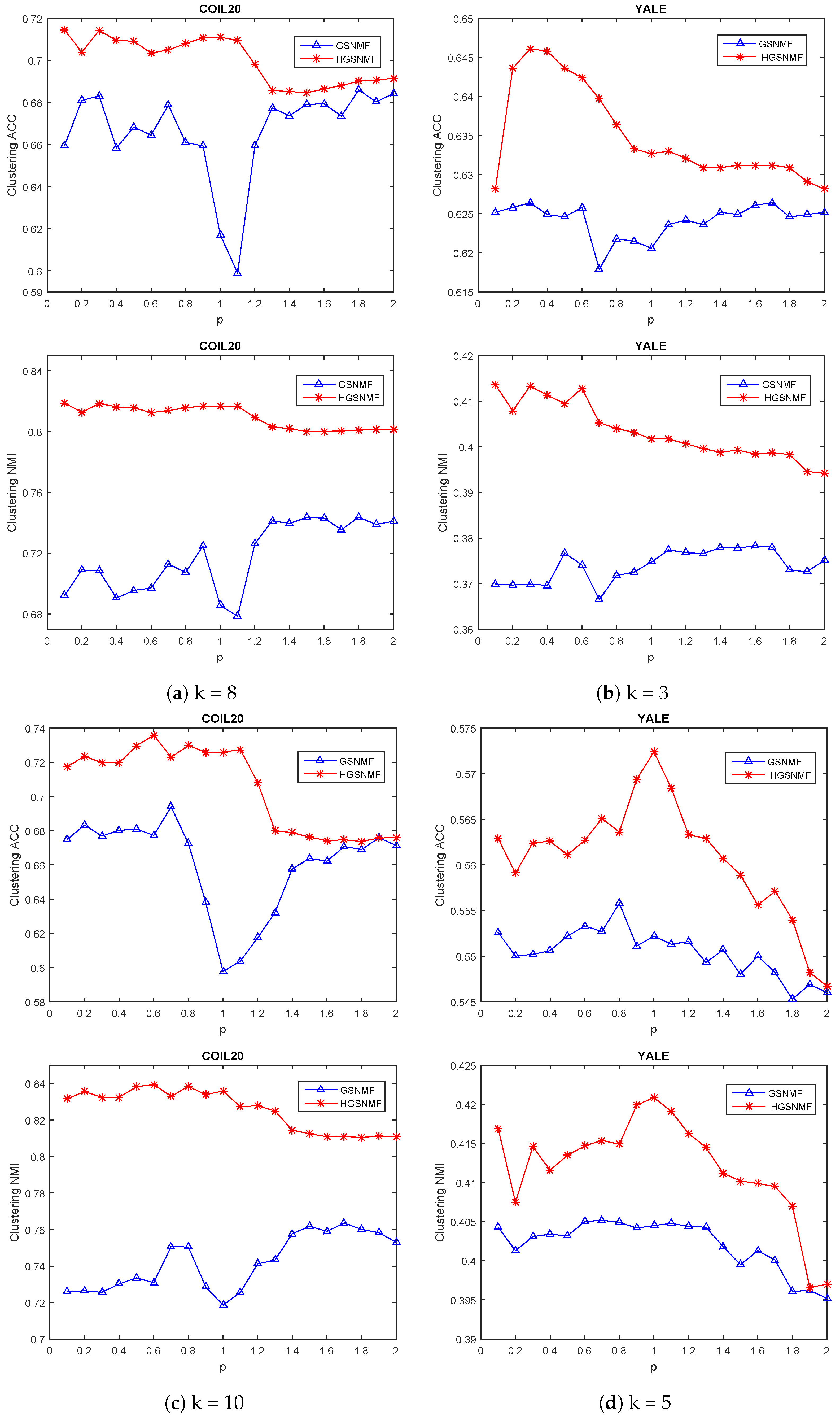
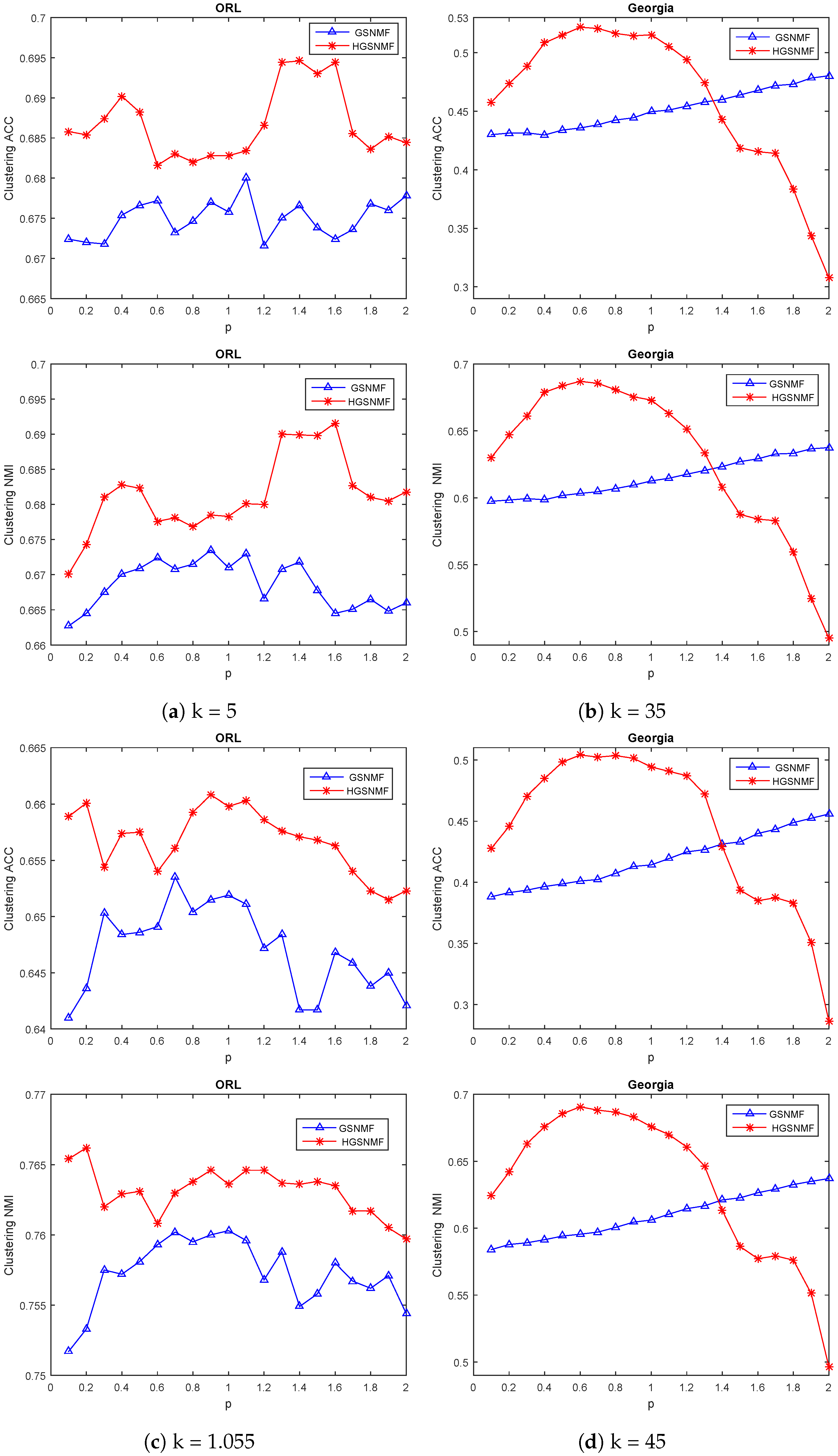
4.4. Parameters Selection

There are three parameters in our proposed HGSNMF algorithm: the regularization parameters α , μ , and p. When α , μ , and p are 0, the proposed HGSNMF method reduces to the NMF [13]; when μ and p are 0, the proposed HGSNMF method reduces to the HNMF [14]. In the experiments, we set k = 5 for all graph-based and hypergraph-based methods for all data sets. To test the effect of each varying parameter, we fixed the other varying parameters as described Section 4.3.
Firstly, we adjusted the parameter α for the GNMF, GSNMF, HNMF, and HGSNMF methods. In the HGSNMF, for k = 4 , we set μ = 100 and p = 1.1 . In the HGSNMF, for k = 8 , we set μ = 1000 and p = 0.3 for the COIL20 data set; for k = 11 and k = 14 , we set μ = 1000 and p = 0.5 for the YALE data set; for k = 20 , we set μ = 1 and p = 1.5 ; for k = 40 , we set μ = 100 and p = 1.5 for the ORL data set; for k = 15 , we set μ = 500 and p = 0.6 ; for k = 20 , we set μ = 1000 and p = 0.5 for the Geogria data set. Figure 2 and Figure 3 demonstrates the accuracy and the normalized mutual information variations with respect to α for four data sets.
As can be seen from Figure 2 and Figure 3, the HGSNMF performed better than the other algorithms in most cases. We can see that the performance of the HGSNMF was relatively stable with respect to the parameter α for some data sets.
Next, we adjusted the parameter μ for the GSNMF and HGSNMF for four data sets, and we set α = 100 and p = 1.7 in the GSNMF. In the HGSNMF, for k = 6 , we set α = 1000 and p = 1.1 ; for k = 12 , we set α = 1000 and 0.5 for the COIL20 data set; for k = 3 , we set α = 500 and p = 0.1 ; for k = 15 , we set α = 500 , α = 1000 , and p = 0.5 for the YALE data set; for k = 15 , we set α = 10 , p = 0.1 ; for k = 25 , we set μ = 1 and p = 1.2 for the ORL data set; for k = 5 and k = 30 , we set μ = 1000 and p = 0.6 for the Georgia data set. As can be seen from Figure 4 and Figure 5, the HGSNMF performed better than the GSNMF in most cases for the four data sets, and the performance of the HGSNMF was stable with respect to the parameter μ for some data sets.
Finally, we considered the variation of the parameter p. In the HGSNMF, for k = 8 , we set α = μ = 1000 ; for k = 10 , we set α = 1000 and μ = 500 for the COIL20 data set; for k = 3 , we set α = 0.1 and μ = 500 ; for k = 5 , we set α = 0.1 and μ = 1000 for the YALE data set; for k = 5 , we set α = μ = 10 , for k = 15 , and we set α = 10 and μ = 1 for the ORL data set; for k = 35 and k = 45 , we set α = 500 and μ = 1000 for the Georgia data set. As shown in Figure 6 and Figure 7, the performance of the HGSNMF was relatively stable and very good with respect to the parameter p varying from 0.1 to 2 for some data sets.
For the Mnist data set, different classes were arbitrarily selected for clustering, and the clustering effects of the seven methods were compared. For the experiments, the graph regularization term parameter was set to 100 in the GNMF, GSNMF, GNTD, and UGNTD, and the hypergraph regularization parameter was set to 100 in the HNMF, HGLNMF, and HGSNMF; µ was also set to 100 in the GSNMF, HGLNMF, and HGSNMF, and the parameter p was set to 1.7 in the GSNMF and HGSNMF. In the GTND and UGNTD, the core tensor was the same as in the experiments in Section 4.3. From Figure 6 and Figure 7, it is clear that our proposed HGSNMF method clustered better than the other methods in most cases with the same selection of parameters on the Mnist data set.
Figure 8 compares performance of GNMF, HNMF, GSNMF, HGLNMF, GNTD, UGNTD, and HGSNMF for number of clusters k for Mnist data set.

4.5. The Converage Analysis

As described in Section 3, the convergence of the proposed HGSNMF method has been proven theoretically. In this section, we analyze the convergence of the proposed method through experiments. Figure 9 shows the convergence curves of our HGSNMF method for three data sets. As can be seen from Figure 9, the objective function was monotonically decreasing and tended to converge after 300 iterations.

5. Conclusions

In this paper, we proposed a hypergraph-regularized L p smooth constrain NMF method for data representation by incorporating the hypergraph regularization term and L p smoothing constraint into NMF. The hypergraph regularization term can better capture the intrinsic geometry structure of high-dimension space data more comprehensively than a simple graph; the L p smoothing constraint may produce a smooth and more accurate solution to the optimization problem. We presented the updating rulers and proved the convergence of our HGSNMF method. Experimental results for five real-world data sets show, as follows, for the COIL20,YALE, ORL, Georgia, and Mnist, the average clustering ACC of our proposed HGSNMF method was more than 1.99 % , 1.89 % , 0.54 % , 3.37 % , and 7.25 % higher than the seconded-best method, respectively, and the average clustering NMI of our proposed HGSNMF method was more than 1.84 % , 2.26 % , 0.6 % , 2.21 % , and 7.21 % higher than the seconded-best method, respectively. Thus, our proposed method can achieve a better clustering effect than other state-of-the-art methods in most cases.
Our HGSNMF method has some limitations: it only considers the hypergraph with high similarity among multiple data points and the smoothness of the basis matrix, and other constraints such as sparse, multiple graphs, and hypergraphs can be considered. The HGSNMF method was only applied to the clustering problem of images. In the future, we can apply hyperspectral mixing, recommended systems, and other aspects. In addition, because the vectorization of the matrix will destroy the internal structure of the data, we will extend to consider nonnegative tensor decomposition in the future.

Author Contributions

Conceptualization, Y.X. and Q.L.; methodology, Y.X. and L.L.; software, Q.L. and Z.C.; writing—original draft preparation, Y.X.; writing—review and editing, Q.L. All authors have read and agreed to the published version of the manuscript.

Funding

This research was partially funded by the National Natural Science Foundation of China under grants 12061025 and 12161020 and partially funded by the Natural Science Foundation of the Educational Commission of Guizhou Province under grants Qian-Jiao-He KY Zi [2019]186, [2019]189, and [2021]298; this research also received funding from the Guizhou Provincial Basis Research Program (Natural Science) (QKHJC[2020]1Z002 and QKHJC-ZK[2023]YB245).

Institutional Review Board Statement

Not applicable.

Informed Consent Statement

Not applicable.

Data Availability Statement

The data presented in this study are available upon request from the corresponding author.

Conflicts of Interest

The authors declare no conflict of interest.

Abbreviations

The following abbreviations are used in this manuscript:
PCAPrincipal component analysis
LDALinear discriminant analysis
SVDSingular value decomposition
NMFNonnegative matrix factorization
HUHyperspectral unmixing
ONMFOrthogonal nonnegative matrix tri-factorizators
GNMFGraph regularized nonnegative matrix factorization
DNMFGraph dual regularization nonnegative matrix factorization
HNMFHypergraph regularized nonnegative matrix factorization
GSNMFGraph regularized L p smooth nonnegative matrix factorization
HGLNMFHypergraph regularized sparse nonnegative matrix factorization
MHGNMFNonnegative matrix factorization with mixed hypergraph regularization
DHPS-NMFDual hypergraph regularized partially shared nonnegative matrix factorization
HGSNMFHypergraph regularized L p smooth nonnegative matrix factorization
ACCAccuracy
NMINormalized mutual information
MIMutual information

References

  1. Pham, N.; Pham, L.; Nguyen, T. A new cluster tendency assessment method for fuzzy co-clustering in hyperspectral image analysis. Neurocomputing 2018, 307, 213–226. [Google Scholar] [CrossRef]
  2. Cai, D.; He, X.; Han, J.; Huang, T. Graph regularized nonnegative matrix factorization for data representation. IEEE Trans. Pattern Anal. Match.Intell. 2011, 33, 1548–1560. [Google Scholar]
  3. Li, S.; Hou, X.; Zhang, H.; Cheng, Q. Learning spatially localized, parts-based representation. In Proceedings of the 2001 IEEE Computer Society Conference on Computer Vision and Pattern Recognition (CVPR 2001), Kauai, HI, USA, 8–14 December 2011; Volume 1, pp. 207–212. [Google Scholar]
  4. He, X.; Yan, S.; Hu, Y.; Niyogi, P.; Zhang, H. Face recognition using laplacian faces. IEEE Trans. Pattern Anal. Mach. Intell. 2005, 27, 328–340. [Google Scholar]
  5. Liu, H.; Wu, Z.; Li, X.; Cai, D.; Huang, T. Constrained nonnegative matrix factorization for image representation. IEEE Trans. Pattern Anal. Mach.Intell. 2011, 34, 1299–1311. [Google Scholar] [CrossRef] [PubMed]
  6. Cutler, A.; Cutler, D.; Stevens, J. Random forests. In Ensemble Machine Learning: Methods and Applications; Springer: Berlin, Germany, 2012; pp. 157–175. [Google Scholar]
  7. Riedmiller, M.; Lernen, A. Multi layer perceptron. In Machine Learning Lab Special Lecture; University of Freiburg: Freiburg, Germany, 2014; pp. 7–24. [Google Scholar]
  8. Wu, L.; Cui, P.; Pei, J. Graph Neural Networks; Springer: Singapore, 2022. [Google Scholar]
  9. Feng, Y.; You, H.; Zhang, Z.; Ji, R.; Gao, Y. Hypergraph neural networks. In Proceedings of the AAAI Conference on Artificial Intelligence, Hilton, HI, USA, 27 January–1 February 2019; Volume 33, pp. 3558–3565. [Google Scholar]
  10. Kirby, M.; Sirovich, L. Application of the karhunen loeve procedure for the characterization of human faces. IEEE Trans. Pattern Anal. Mach. Intell. 1990, 12, 103–108. [Google Scholar] [CrossRef] [Green Version]
  11. Strang, G. Introduction to Linear Algebra; Wellesley-Cambridge: Wellesley, MA, USA, 2009. [Google Scholar]
  12. Martinez, A.; Kak, A. Pca versus lda. IEEE Trans. Pattern Anal. Mach. Intell. 2001, 23, 228–233. [Google Scholar] [CrossRef] [Green Version]
  13. Lee, D.; Seung, H. Learning of the parts of objects by non-negative matrix factorization. Nature 1999, 401, 788–791. [Google Scholar] [CrossRef]
  14. Lee, D.; Seung, H. Algorithms for nonnegative matrix factorization. In Proceedings of the International Conference on Neural Information Processing Systems, Denver, CO, USA, 28–30 November 2000; Volume 13, pp. 556–562. [Google Scholar]
  15. Tucker, L. Some mathematical notes on three-mode factor analysis. Psychometrika 1966, 31, 279–311. [Google Scholar] [CrossRef]
  16. Kim, Y.; Choi, S. Nonnegative Tucker decomposition. In Proceedings of the 2007 IEEE Conference on Computer Vision and Pattern Recognition, Minneapolis, MN, USA, 17–22 June 2007; pp. 1–8. [Google Scholar]
  17. Kolda, T.; Bader, B. Tensor decompositions and applications. SIAM Rev. 2009, 51, 455–500. [Google Scholar] [CrossRef]
  18. Che, M.; Wei, Y.; Yan, H. An efficient randomized algorithm for computing the approximate tucker decomposition. J. Sci. Comput. 2021, 88, 1–29. [Google Scholar] [CrossRef]
  19. Pan, J.; Ng, M.; Liu, Y.; Zhang, X.; Yan, H. Orthogonal nonnegative Tucker decomposition. SIAM J. Sci. Comput. 2021, 43, B55–B81. [Google Scholar] [CrossRef]
  20. Ding, C.; He, X.; Simon, H. On the equivalence of nonnegative matrix factorization and spectral clustering. In Proceedings of the 2005 SIAM International Conference on Data Mining (SDM05), Newport Beach, CA, USA, 21–23 April 2005; pp. 606–610. [Google Scholar]
  21. Ding, C.; Li, T.; Peng, W.; Park, H. Orthogonal nonnegative matrix tri-factorizations for clustering. In Proceedings of the 12th ACM SIGKDD International Conference on Knowledge Discovery and Data Mining, Philadelphia, PA, USA, 20–23 August 2006; pp. 126–135. [Google Scholar]
  22. Pan, J.; Ng, M. Orthogonal nonnegative matrix factorization by sparsity and nuclear norm optimization. SIAM. J. Matrix Anal. Appl. 2018, 39, 856–875. [Google Scholar] [CrossRef]
  23. Guillamet, D.; Vitria, J.; Schiele, B. Introducing a weighted nonnegative matrix factorization for image classification. Pattern Recognit. Lett. 2003, 24, 2447–2454. [Google Scholar] [CrossRef]
  24. Tan, X.; Triggs, B. Enhanced local texture feature sets for face recognition under difficult lighting conditions. IEEE Trans. Image Process. 2010, 19, 1635–1650. [Google Scholar]
  25. Pauca, V.; Shahnaz, F.; Berry, M.; Plemmons, R. Text mining using nonnegative matrix factorizations. SIAM. Int. Conf. Data Min. 2004, 4, 452–456. [Google Scholar]
  26. Li, T.; Ding, C. The relationships among various nonnegative matrix factorization methods for clustering. IEEE. Comput. Soci. 2006, 4, 362–371. [Google Scholar]
  27. Liu, Y.; Jing, L.; Ng, M. Robust and non-negative collective matrix factorization for text-to-image transfer learning. IEEE Trans. Image Process. 2015, 24, 4701–4714. [Google Scholar]
  28. Gillis, N. Sparse and unique nonnegative matrix factorization through data preprocessing. J. Mach. Learn. Res. 2012, 1, 3349–3386. [Google Scholar]
  29. Gillis, N. Nonnegative Matrix Factorization; SIAM: Philadelphia, PA, USA, 2020. [Google Scholar]
  30. Wang, W.; Qian, Y.; Tan, Y. Hypergraph-regularized spares NMF for hyperspectral unmixing. IEEE J. Sel. Topi. Appl. Earth. Obs. Remot Sens. 2016, 9, 681–694. [Google Scholar] [CrossRef]
  31. Ma, Y.; Li, C.; Mei, X.; Liu, C.; Ma, J. Robust sparse hyperspectral unmixing withL2,1 norm. IEEE Trans. Geosci. Remot Sens. 2017, 55, 1227–1239. [Google Scholar] [CrossRef]
  32. Li, Z.; Liu, J.; Lu, H. Structure preserving non-negative matrix factorization for dimensionality reduction. Comput. Vis. Image Underst. 2013, 117, 1175–1189. [Google Scholar] [CrossRef]
  33. Luo, X.; Zhou, M.; Leung, H.; Xia, Y.; Zhu, Q.; You, Z.; Li, S. An incremental-and-static-combined scheme for matrix-factorization- based collaborative filtering. IEEE Trans. Autom. Sci. Eng. 2014, 13, 333–343. [Google Scholar] [CrossRef]
  34. Zhou, G.; Yang, Z.; Xie, S.; Yang, J. Online blind source separation using incremental nonnegative matrix factorization with volume constraint. IEEE Trans. Neur. Netw. 2011, 22, 550–560. [Google Scholar] [CrossRef] [PubMed]
  35. Pan, J.; Gillis, N. Generalized separable nonnegative matrix factorization. IEEE Trans. Pattern Anal. Mach. Intell. 2021, 43, 1546–1561. [Google Scholar] [CrossRef] [PubMed]
  36. Shang, F.; Jiao, L.; Wang, F. Graph dual regularization nonnegative matrix factorization for co-clustering. Pattern Recognit. 2012, 45, 2237–2250. [Google Scholar] [CrossRef]
  37. Zeng, K.; Jun, Y.; Wang, C.; You, J.; Jin, T. Image clustering by hypergraph regularized nonnegatve matrix factorization. Neurocomputing 2014, 138, 209–217. [Google Scholar] [CrossRef]
  38. Leng, C.; Zhang, H.; Cai, G.; Cheng, I.; Basu, A. Graph regularized Lp smooth nonnegative matrix factorization for data representation. IEEE/CAA J. Autom. 2019, 6, 584–595. [Google Scholar] [CrossRef]
  39. Qiu, Y.; Zhou, G.; Zhang, Y.; Xie, S. Graph regularized nonnegative tucker decomposition for tensor data representation. In Proceedings of the IEEE International Conference on Acoustics, Speech and Signal Processing (ICASSP), Brighton, UK, 12–17 May 2019; pp. 8613–8617. [Google Scholar]
  40. Qiu, Y.; Zhou, G.; Wang, Y.; Zhang, Y.; Xie, S. A generalized graph regularized non-negative Tucker decomposition framework for tensor data representation. IEEE Trans. Cybern. 2022, 52, 594–607. [Google Scholar] [CrossRef]
  41. Wood, G.; Jennings, L. On the use of spline functions for data smoothing. J. Biomech. 1979, 12, 477–479. [Google Scholar] [CrossRef]
  42. Lyons, J. Differentiation of solutions of nonlocal boundary value problems with respect to boundary data. Electron. J. Qual. Theory Differ. Equ. 2001, 51, 1–11. [Google Scholar] [CrossRef]
  43. Xu, L. Data smoothing regularization, multi-sets-learning, and problem solving strategies. Neural Netw. 2003, 16, 817–825. [Google Scholar] [CrossRef] [PubMed]
  44. Zhou, D.; Huang, J.; Scholkopf, B. Learning with Hypergraphs: Clustering, Classification, and Embdding; MIT Press: Cambridge, MA, USA, 2006; Volume 19, pp. 1601–1608. [Google Scholar]
  45. Gao, Y.; Zhang, Z.; Lin, H.; Zhao, X.; Du, S.; Zou, C. Hypergraph learning: Methods and practices. IEEE Trans. Pattern Anal. Mach. Intell. 2020, 44, 2548–2566. [Google Scholar] [CrossRef] [PubMed]
  46. Huan, Y.; Liu, Q.; Lv, F.; Gong, Y.; Metaxax, D. Unsupervised image categorization by hypergraph partition. IEEE Trans. Pattern Anal. Mach. Intell. 2011, 33, 17–24. [Google Scholar]
  47. Yu, J.; Tao, D.; Wang, M. Adaptive hypergraph learning and its application in image classification. IEEE Trans. Image Process. 2012, 21, 3262–3272. [Google Scholar] [PubMed]
  48. Hong, C.; Yu, J.; Li, J.; Chen, X. Multi-view hypergraph learning by patch alignment framework. Neurocomputing 2013, 118, 79–86. [Google Scholar] [CrossRef]
  49. Wang, C.; Yu, J.; Tao, D. High-level attributes modeling for indoor scenes classifiation. Neurocomputing 2013, 121, 337–343. [Google Scholar] [CrossRef]
  50. Chen, C.; Liu, Y. A survey on hyperlink prediction. arXiv 2022, arXiv:2207.02911. [Google Scholar]
  51. Yin, W.; Qu, Y.; Ma, Z.; Liu, Q. Hyperntf: A hypergraph regularized nonnegative tensor factorization for dimensionality reduction. Neurocomputing 2022, 512, 190–202. [Google Scholar] [CrossRef]
  52. Wu, W.; Kwong, S.; Zhou, Y. Nonnegative matrix factorization with mixed hypergraph regularization for community detection. Inf. Sci. 2018, 435, 263–281. [Google Scholar] [CrossRef]
  53. Zhang, D. Semi-supervised multi-view clustering with dual hypergraph regularized partially shared nonnegative matrix factorization. Sci. China Technol. Sci. 2022, 65, 1349–1365. [Google Scholar] [CrossRef]
  54. Huang, H.; Zhou, G.; Liang, N.; Zhao, Q.; Xie, S. Diverse deep matrix factorization with hypergraph regularization for multiview data representation. IEEE/CAA J. Autom. Sin. 2022, 34, 1–44. [Google Scholar] [CrossRef]
  55. Cai, D.; He, X.; Han, J. Documen clustering using locality preserving indexing. IEEE Trans. Knowl. Data Eng. 2005, 17, 1624–1637. [Google Scholar] [CrossRef] [Green Version]
  56. Lovasz, L.; Plummer, M. Matching Theory; American Mathematical Society: Providence, RI, USA, 2009; Volume 367. [Google Scholar]
Figure 1. An illustration of the simple graph, the hypergraph G ¯ , and an indication matrix.
Mathematics 11 02821 g001
Figure 2. Performance comparison of GNMF, HNMF, GSNMF, and HGSNMF for varying the parameter α . Each column indicates the COIL20 and YALE data sets.
Mathematics 11 02821 g002
Figure 3. Performance comparison of GNMF, HNMF, GSNMF, and HGSNMF for varying the parameter α . Each column indicates the for ORL and Georgia data sets.
Mathematics 11 02821 g003
Figure 4. Performance comparison of GSNMF and HGSNMF for varying parameter μ . Each column indicates the COIL20 and YALEdata sets.
Mathematics 11 02821 g004
Figure 5. Performance comparison of GSNMF and HGSNMF for varying parameter μ . Each column indicates the ORL and Georgia data sets.
Mathematics 11 02821 g005
Figure 6. Performance comparison of GSNMF, and HGSNMF for varying parameter p for COIL20 and YALEdata sets.
Mathematics 11 02821 g006
Figure 7. Performance comparison of GSNMF, and HGSNMF for varying parameter p forORL and Georgia data sets.
Mathematics 11 02821 g007
Figure 8. Performance comparison of GNMF, HNMF, GSNMF, HGLNMF, GNTD, UGNTD, and HGSNMF for number of clusters k for Mnist data set.
Mathematics 11 02821 g008
Figure 9. The relative residuals versus the number of iterations for HGSNMF for four data sets.
Mathematics 11 02821 g009
Table 1. Computational operation counts for each iteration in NMF, GNMF, HNMF, GSNMF, HGLNMF, and HGSNMF.
fladdflmltfldivOverall
NMF 2 n m r + 2 ( m + n ) r 2 2 n m r +2 ( m + n ) r 2 + m r + n r m r + n r O ( m n r )
GNMF2 n m r +2 ( m + n ) r 2 + n r + 3 n 2 n m r +2 ( m + n ) r 2 + ( m + 2 n + n k ) r m r + n r O ( m n r )
HNMF2 n m r +2 ( m + n ) r 2 + n r + 3 n 2 n m r +2 ( m + n ) r 2 + ( m + 2 n + n k ) r m r + n r O ( m n r )
GSNMF2 n m r +2 ( m + n ) r 2 + n k + 3 n + m r 2 n m r +2 ( m + n ) r 2 + ( m + 2 n + n k ) r m r + n r O ( m n r )
HGLNMF2 n m r +2 ( m + n ) r 2 + n k + 3 n + m r 2 n m r +2 ( m + n ) r 2 + ( m + 2 n + n k ) r m r + n r O ( m n r )
HGSNMF2 n m r +2 ( m + n ) r 2 + n k + 3 n + m r 2 n m r +2 ( m + n ) r 2 + ( m + 2 n + n k ) r m r + n r O ( m n r )
Table 2. Statistics of the five data sets.
Data SetsSamplesFeaturesClasses
COIL201440102420
YALE165102415
ORL400102440
Georgia750102450
Mnist50078410
Table 3. Normalized mutual information (NMI) on COIL20 data set.
kK-MeansNMFGNMFHNMFGSNMFHGLNMFHGSNMF
465.13 ± 16.6069.63 ± 15.7672.86 ± 14.8679.53 ± 13.6573.79 ± 13.5179.52 ± 13.64 84 . 45 ± 15 . 24
667.70 ± 9.7969.65 ± 11.2772.79 ± 10.7080.72 ± 10.5868.63 ± 10.0080.76 ± 10.54 83 . 84 ± 8 . 37
870.56 ± 5.8969.44 ± 8.7871.53 ± 8.6080.94 ± 7.3573.55 ± 7.2881.08 ± 7.38 81 . 85 ± 8 . 11
1076.02 ± 7.1270.13 ± 6.9576.01 ± 5.4882.99 ± 5.8476.36 ± 5.9283.00 ± 5.75 83 . 83 ± 5 . 41
1273.21 ± 4.8270.91 ± 5.5077.12 ± 5.6882.16 ± 5.0375.70 ± 5.3382.31 ± 5.08 83 . 75 ± 5 . 31
1474.10 ± 4.3170.41 ± 4.6677.06 ± 4.7582.20 ± 4.2476.88 ± 4.6382.21 ± 4.19 83 . 69 ± 4 . 78
1674.85 ± 3.6572.70 ± 4.0479.38 ± 4.5284.05 ± 3.9579.04 ± 4.2783.99 ± 3.97 85 . 83 ± 4 . 28
1873.28 ± 3.0871.49 ± 3.0078.03 ± 3.6584.61 ± 3.1579.36 ± 3.4784.70 ± 3.16 85 . 74 ± 3 . 30
2073.83 ± 2.5271.95 ± 2.7679.20 ± 3.0584.08 ± 2.7978.84 ± 2.7684.05 ± 2.71 85 . 15 ± 3 . 52
Avg.72.071.7076.0082.3675.8082.40 84 . 24
Table 4. Clustering accuracy (ACC) on COIL20 data set.
kK-MeansNMFGNMFHNMFGSNMFHGLNMFHGSNMF
471.45 ± 14.8272.35 ± 16.5073.41 ± 14.8575.78 ± 17.8875.33 ± 15.7475.77 ± 17.88 81 . 31 ± 19 . 19
667.05 ± 10.7268.87 ± 11.8069.65 ± 12.6174.42 ± 13.7868.04 ± 10.7874.44 ± 13.78 77 . 30 ± 11 . 89
864.56 ± 64.5665.39 ± 9.9564.35 ± 10.9371.06 ± 11.7767.36 ± 9.7370.71 ± 11.75 71 . 43 ± 11 . 74
1067.38 ± 9.7663.27 ± 7.9666.76 ± 7.4770.73 ± 10.0467.07 ± 8.4470.61 ± 5.75 73 . 39 ± 8 . 96
1263.73 ± 7.0963.19 ± 7.0266.81 ± 8.3068.63 ± 8.4365.81 ± 8.4369.00 ± 5.08 71 . 50 ± 8 . 22
1462.48 ± 6.4260.01 ± 6.1665.18 ± 7.5768.04 ± 8.3364.21 ± 7.7768.03 ± 8.18 83 . 69 ± 7 . 88
1661.78 ± 5.6962.18 ± 6.4365.47 ± 7.2569.09 ± 7.6266.03 ± 7.5068.85 ± 7.66 70 . 31 ± 8 . 24
1859.15 ± 6.1859.68 ± 5.4463.39 ± 6.8669.29 ± 6.5165.84 ± 6.7069.65 ± 6.59 70 . 85 ± 6 . 35
2058.18 ± 5.4359.11 ± 4.6063.86 ± 6.24 68 . 68 ± 6 . 52 63.95 ± 6.0068.56 ± 6.3468.19 ± 6.83
Avg.63.9763.7866.5470.6467.0770.63 72 . 63
Table 5. Normalized mutual information (NMI) on YALE data set.
kK-MeansNMFGNMFHNMFGSNMFHGLNMFHGSNMF
340.18 ± 23.0328.96 ± 11.7128.81 ± 12.0636.08 ± 12.8237.80 ± 16.4036.12 ± 12.89 41 . 36 ± 13 . 07
535.72 ± 12.8738.23 ± 10.2538.48 ± 10.0239.37 ± 8.8340.01 ± 10.6139.35 ± 8.85 41 . 91 ± 10 . 34
7 43 . 18 ± 6 . 55 38.38 ± 6.5138.17 ± 7.5739.07 ± 6.8439.33 ± 6.4639.38 ± 5.2342.32 ± 7.39
9 42 . 22 ± 7 . 98 41.80 ± 3.8740.56 ± 5.0038.93 ± 5.0538.85 ± 4.8839.18 ± 5.2340.21 ± 4.35
1139.80 ± 4.4041.82 ± 4.4542.05 ± 4.2543.88 ± 4.3044.08 ± 4.6244.04 ± 4.61 45 . 06 ± 4 . 70
1344.13 ± 4.6344.17 ± 3.0344.59 ± 3.4344.24 ± 3.1244.53 ± 2.8044.29 ± 3.07 47 . 54 ± 3 . 84
1444.34 ± 3.8443.27 ± 2.9243.31 ± 3.1044.21 ± 3.3944.82 ± 3.0244.21 ± 3.32 46 . 82 ± 3 . 85
1544.48 ± 2.9243.91 ± 2.9044.36 ± 2.7245.37 ± 2.3845.32 ± 2.6245.47 ± 2.35 47 . 60 ± 3 . 06
Avg.41.7640.0740.0441.4041.8441.51 44 . 10
Table 6. Clustering accuracy (ACC) on YALE data set.
kK-MeansNMFGNMFHNMFGSNMFHGLNMFHGSNMF
362.24 ± 14.9159.30 ± 8.1659.12 ± 8.1161.49 ± 8.2062.64 ± 11.1461.91 ± 8.61 64 . 82 ± 10 . 06
550.24 ± 10.6654.15 ± 8.9253.78 ± 8.2754.95 ± 7.8354.82 ± 9.0454.84 ± 7.82 56 . 84 ± 8 . 79
749.43 ± 6.2647.40 ± 6.3346.92 ± 6.9047.21 ± 6.8146.65 ± 6.1447.44 ± 6.62 49 . 87 ± 7 . 32
944.40 ± 7.02 44 . 87 ± 4 . 30 43.12 ± 4.8742.48 ± 5.4542.15 ± 4.7442.81 ± 5.4943.68 ± 4.98
1139.12 ± 4.8041.37 ± 5.0641.74 ± 4.6543.43 ± 5.0043.07 ± 5.2943.50 ± 5.12 44 . 19 ± 5 . 20
1340.41 ± 4.8141.18 ± 3.7341.11 ± 4.1040.76 ± 3.8341.05 ± 3.6140.78 ± 3.91 43 . 57 ± 4 . 17
1439.46 ± 4.2639.05 ± 4.2138.27 ± 3.7239.92 ± 4.2140.03 ± 3.7539.94 ± 4.22 41 . 97 ± 4 . 33
1538.52 ± 3.3038.72 ± 3.5138.67 ± 3.2140.25 ± 3.3939.52 ± 3.1440.44 ± 3.24 41 . 86 ± 3 . 37
Avg.45.4145.7645.3446.3146.2446.46 48 . 35
Table 7. Normalized mutual information (NMI) on ORL data set.
kK-MeansNMFGNMFHNMFGSNMFHGLNMFHGSNMF
566.24 ± 12.0067.18 ± 12.0768.81 ± 11.1668.58 ± 12.7766.51 ± 13.1868.97 ± 13.01 68 . 98 ± 12 . 29
1070.22 ± 6.6373.59 ± 5.90 73 . 72 ± 7 . 10 72.11 ± 6.7071.95 ± 5.9272.39 ± 6.5973.29 ± 6.55
1568.46 ± 4.2175.23 ± 5.0176.14 ± 5.1875.26 ± 5.6275.67 ± 5.2775.26 ± 5.62 76 . 54 ± 5 . 42
2069.87 ± 4.7574.21 ± 4.3474.44 ± 4.7875.24 ± 4.2575.49 ± 3.7675.46 ± 4.19 76 . 00 ± 4 . 08
2571.13 ± 3.4875.51 ± 2.6975.88 ± 3.1376.03 ± 3.2976.10 ± 3.1776.06 ± 3.12 76 . 91 ± 3 . 22
3071.03 ± 2.8175.34 ± 3.1275.55 ± 2.8174.60 ± 2.67 75 . 89 ± 2 . 78 74.69 ± 2.6575.88 ± 2.80
3571.07 ± 1.8275.07 ± 2.2374.96 ± 2.0674.46 ± 1.8775.85 ± 2.1874.52 ± 1.91 75 . 96 ± 2 . 35
4071.45 ± 2.0675.05 ± 1.9075.26 ± 1.8274.54 ± 1.8775.40 ± 1.9174.54 ± 1.91 76 . 07 ± 1 . 77
Avg.69.9373.9074.3573.8574.1173.99 74 . 95
Table 8. Clustering accuracy (ACC) on ORL data set.
kK-MeansNMFGNMFHNMFGSNMFHGLNMFHGSNMF
567.32 ± 14.9168.12 ± 12.1168.76 ± 12.3168.70 ± 12.2767.36 ± 12.7268.97 ± 13.01 69 . 30 ± 12 . 15
1062.72 ± 10.66 66 . 11 ± 8 . 02 65.85 ± 9.8664.05 ± 7.8764.59 ± 7.2264.46 ± 7.8265.42 ± 7.50
1556.19 ± 5.8063.55 ± 6.8564.84 ± 6.9663.99 ± 7.4464.59 ± 7.3263.99 ± 7.44 65 . 89 ± 7 . 38
2055.29 ± 6.2561.21 ± 5.8361.56 ± 6.2162.44 ± 5.8762.67 ± 5.3062.52 ± 5.57 62 . 80 ± 5 . 73
2554.15 ± 4.5060.58 ± 3.9861.01 ± 4.8461.31 ± 4.6661.16 ± 4.9661.32 ± 4.80 61 . 91 ± 5 . 22
3052.52 ± 4.2958.57 ± 4.6758.88 ± 4.5258.07 ± 4.42 59 . 91 ± 4 . 08 58.38 ± 4.2859.50 ± 4.20
3551.30 ± 3.2057.83 ± 3.6257.22 ± 3.4656.95 ± 3.28 58 . 79 ± 3 . 58 57.05 ± 3.2158.35 ± 4.06
4050.68 ± 3.4356.57 ± 3.3956.73 ± 3.1555.88 ± 3.3257.20 ± 3.4655.88 ± 3.37 57 . 36 ± 3 . 38
Avg.56.2761.5761.8661.4262.0361.57 62 . 57
Table 9. Normalized mutual information (NMI) on Georgia data set.
kK-MeansNMFGNMFHNMFGSNMFHGLNMFHGSNMF
567.05 ± 11.3359.40 ± 11.7963.00 ± 12.2760.93 ± 11.9364.46 ± 10.8360.99 ± 11.94 68 . 18 ± 9 . 19
10 67 . 82 ± 7 . 48 60.25 ± 8.9361.24 ± 8.5157.48 ± 10.5061.59 ± 10.1257.63 ± 10.6765.91 ± 9.15
1564.64 ± 5.3260.57 ± 4.3962.46 ± 4.8561.89 ± 5.1264.02 ± 5.7261.99 ± 5.02 68 . 55 ± 5 . 08
2067.12 ± 4.3060.60 ± 3.7162.58 ± 3.9160.98 ± 3.8164.44 ± 3.1861.08 ± 3.82 68 . 91 ± 2 . 93
2566.30 ± 3.3159.31 ± 2.7361.35 ± 2.6261.33 ± 3.2264.83 ± 2.9861.32 ± 3.68 69 . 44 ± 2 . 87
3066.01 ± 3.1360.26 ± 2.5663.20 ± 2.2560.52 ± 3.0464.61 ± 2.9760.47 ± 2.99 69 . 61 ± 2 . 87
3565.10 ± 2.1359.93 ± 2.3363.3 ± 1.8059.21 ± 2.2163.27 ± 2.3759.20 ± 2.22 68 . 70 ± 1 . 95
4066.06 ± 2.2059.58 ± 2.3462.84 ± 1.8258.61 ± 2.3863.57 ± 1.9858.62 ± 2.48 69 . 18 ± 1 . 69
4566.17 ± 1.3559.99 ± 1.7562.92 ± 1.5558.22 ± 1.9062.92 ± 1.6658.25 ± 1.99 69 . 07 ± 1 . 41
5066.36 ± 1.3259.05 ± 1.5662.11 ± 1.5158.19 ± 1.3363.18 ± 1.2458.19 ± 1.25 69 . 18 ± 1 . 13
Avg.66.2659.9062.5059.7463.6959.77 68 . 47
Table 10. Clustering accuracy (ACC) on Georgia data set.
kK-MeansNMFGNMFHNMFGSNMFHGLNMFHGSNMF
568.73 ± 11.5066.68 ± 10.9669.52 ± 11.1568.00 ± 10.3369.76 ± 10.5067.68 ± 10.47 73 . 12 ± 10 . 04
1061.71 ± 8.5657.79 ± 8.4859.25 ± 8.4455.73 ± 9.0959.07 ± 8.9455.83 ± 9.23 61 . 97 ± 9 . 39
1555.38 ± 6.2753.33 ± 4.4155.05 ± 5.3855.07 ± 5.4156.08 ± 6.1555.21 ± 5.38 59 . 40 ± 6 . 31
2055.14 ± 5.0750.55 ± 4.5852.30 ± 4.6050.22 ± 4.4554.93 ± 4.3650.37 ± 4.40 57 . 50 ± 4 . 29
2551.82 ± 4.4046.8¡¤ ± 3.5948.50 ± 3.4248.25 ± 4.3852.10 ± 4.0948.311 ± 4.30 55 . 52 ± 4 . 06
3049.67 ± 4.1245.20 ± 3.4948.31 ± 3.1345.82 ± 3.4850.17 ± 3.8245.68 ± 3.33 54 . 18 ± 3 . 67
3547.80 ± 3.2843.78 ± 3.1247.09 ± 2.9242.57 ± 3.0347.19 ± 3.3142.53 ± 3.02 52 . 17 ± 2 . 96
4047.88 ± 3.2841.93 ± 2.9545.35 ± 2.8140.47 ± 3.2646.27 ± 3.0240.41 ± 3.45 51 . 52 ± 2 . 90
4547.39 ± 2.2641.07 ± 2.5243.93 ± 2.4438.53 ± 2.4944.34 ± 2.5038.58 ± 2.59 50 . 40 ± 2 . 50
5046.18 ± 2.1938.94 ± 2.2242.14 ± 2.4037.24 ± 1.9243.78 ± 2.3237.26 ± 1.90 49 . 62 ± 2 . 45
Avg.53.1748.6151.1448.1952.3748.19 56 . 54
Table 11. Normalized mutual information (NMI) on Mnist data set.
kGNMFHNMFGSNMFHGLNMFGNTDUGNTDHGSNMF
258.89 ± 23.9457.08 ± 24.3842.94 ± 12.9157.34 ± 24.2767.11 ± 18.2753.17 ± 36.19 71 . 18 ± 28 . 49
453.12 ± 12.6755.64 ± 14.5153.70 ± 12.2655.61 ± 14.0457.17 ± 11.6056.32 ± 11.42 68 . 09 ± 13 . 31
645.17 ± 4.9049.23 ± 5.8548.53 ± 6.1148.72 ± 5.9949.20 ± 5.0156.27 ± 7.69 61 . 57 ± 7 . 43
747.63 ± 6.8245.51 ± 4.8247.48 ± 4.4846.88 ± 5.4647.05 ± 5.1455.69 ± 7.31 59 . 52 ± 6 . 56
848.55 ± 3.8648.32 ± 4.3849.76 ± 4.8747.22 ± 3.8347.38 ± 3.3857.30 ± 6.01 61 . 25 ± 3 . 97
1047.01 ± 4.3945.06 ± 2.2146.30 ± 3.6544.46 ± 2.8145.07 ± 4.0856.11 ± 4.73 57 . 92 ± 3 . 59
Avg.50.0650.1448.1250.0452.1655.81 63 . 26
Table 12. Clustering accuracy (ACC) on Mnist data set.
kGNMFHNMFGSNMFHGLNMFGNTDUGNTDHGSNMF
280.07 ± 28.0587.96 ± 13.1780.50 ± 17.5588.13 ± 12.96 92 . 51 ± 5 . 32 82.73 ± 17.2891.57 ± 13.32
470.89 ± 11.2874.17 ± 12.6771.51 ± 16.9365.99 ± 24.92 75 . 26 ± 10 . 35 67.74 ± 11.5071.32 ± 26.19
657.26 ± 5.4860.41 ± 7.0657.58 ± 7.3759.36 ± 7.6460.50 ± 6.7444.47 ± 21.53 65 . 06 ± 9 . 44
757.52 ± 7.6654.99 ± 5.8454.82 ± 3.9755.54 ± 5.6955.68 ± 5.2456.34 ± 7.57 62 . 74 ± 7 . 98
845.34 ± 2.0855.63 ± 5.1856.84 ± 5.2749.11 ± 15.9155.21 ± 4.34 58 . 01 ± 6 . 34 56.78 ± 19.12
1050.72 ± 5.4248.21 ± 3.6848.28 ± 6.0548.02 ± 4.0047.93 ± 4.5351.01 ± 6.48 56 . 41 ± 5 . 09
Avg.60.3063.5661.5960.8660.0568 67 . 31
Table 13. Comparisons of computation time in the YALE.
kNMFGNMFHNMFGSNMFHGLNMFHGSNMF
3 0 . 88 1.152.513.144.083.15
11 5 . 22 9.2120.7521.3135.6214.77
13 10 . 29 17.6341.1242.1867.8928.70
14 12 . 13 20.6449.8046.7580.0635.45
15 13 . 39 22.5255.3554.1896.9443.62
Table 14. Comparisons of computation time in the Georgia.
kNMFGNMFHNMFGSNMFHGLNMFHGSNMF
10 9 . 19 25.3947.7935.7769.745.07
15 16 . 94 40.3694.5767.58134.6788.01
20 24 . 57 56.96123.3089.73183.88120.07
25 40 . 84 90.97233.04151.94312.03201.96
30 55 . 86 114.43343.62196.97429.94214.84
Disclaimer/Publisher’s Note: The statements, opinions and data contained in all publications are solely those of the individual author(s) and contributor(s) and not of MDPI and/or the editor(s). MDPI and/or the editor(s) disclaim responsibility for any injury to people or property resulting from any ideas, methods, instructions or products referred to in the content.

