A Protocol for Solutions to DP-Complete Problems through Tissue Membrane Systems

Abstract

Considering a class $\mathcal{R}$ comprising recognizer membrane systems with the capability of providing polynomial-time and uniform solutions for NP-complete problems (referred to as a “presumably efficient” class), the corresponding polynomial-time complexity class PMC${}_{\mathcal{R}}$ encompasses both the NP and $\mathbf{co}-\mathbf{NP}$ classes. Specifically, when $\mathcal{R}$ represents the class of recognizer presumably efficient cell-like P systems that incorporate object evolution rules, communication rules, and dissolution rules, PMC${}_{\mathcal{R}}$ includes both the DP and $\mathbf{co}-\mathbf{DP}$ classes. Here, DP signifies the class of languages that can be expressed as the difference between any two languages in NP (it is worth noting that NP ⊆ DP and $\mathbf{co}-\mathbf{NP}\subseteq \mathbf{co}-\mathbf{DP}$). As DP-complete problems are believed to be more complex than NP-complete problems, they serve as promising candidates for studying the P vs. NP problem. This outcome has previously been established within the realm of recognizer P systems with active membranes. In this paper, we extend this result to encompass any class $\mathcal{R}$ of presumably efficient recognizer tissue-like membrane systems by presenting a detailed protocol for transforming solutions of NP-complete problems into solutions of DP-complete problems.

1. Introduction

Roughly speaking, a mechanical procedure consists of a set of elementary tasks, possibly repeated, structured by a total order. A mechanical solution of an abstract problem is a mechanical procedure such that the execution of the corresponding tasks in the order prefixed by the procedure provides the correct solution of the problem. A computing model basically consists of a formal/mathematical definition of the intuitive concept of mechanical procedure. Consequently, in a computing model will be possible to define in a rigorous way what solving an abstract problem through a mechanical way means. A computing paradigm is a mathematical theory that allows us to consider computing models satisfying some syntactic and/or semantic properties previously established in the theory.

Membrane Computing is a branch of Natural Computing introduced by Gh. Păun at the end of 1998 [1]. It is a computing paradigm inspired by the architecture and the functioning of living cells, as well as from the way the cells are organized in tissues, organs or other higher-order structures. This paradigm provides distributed, parallel non-deterministic computing models whose computational devices are generically called membrane systems. This paper deals with tissue-like membrane systems inspired by the cell inter-communication in tissues, where the processor units, called cells, are considered to be the nodes of a directed graph. In this context, cells can communicate through some kind of rewriting rules (called symport/antiport rules), which were introduced in membrane computing in [2]. The basic concept of tissue P systems [3,4] gave rise to several research lines and variants: see, for example [5,6,7]. These systems can present cooperative behavior in the following sense: two or more objects can interact to fire a rule. It can be seen in rules where two or more objects are necessary to be executed. Replication stands as a fundamental function within a cell, where, under optimal conditions, cell division (mitosis) yields two identical copies. Drawing inspiration from this phenomenon, cell division rules were incorporated into the framework of tissue P systems. These rules serve as a mechanism for generating an exponential workspace in terms of the number of objects and cells involved. By employing such rules, the two newly formed cells resulting from the division process contain precisely the same objects, differing at most by a pair of distinct objects.

It is a well-established fact that every decision problem can be associated with a language in a manner that solving the decision problem corresponds to recognizing the “corresponding” language. In the field of Membrane Computing, the concept of “Recognizer membrane systems” was introduced in [8] as a natural framework for solving decision problems through language recognition. A membrane system is considered a recognizer if it exhibits specific syntactic and semantic characteristics: (a) The working alphabet comprises two distinguished objects, namely, yes and no. (b) There exists an input alphabet that is strictly contained within the working alphabet, along with an input “compartment” (a distinguished membrane in the case of cell-like devices, or a distinguished cell in the case of tissue-like devices). (c) The initial content of each cell consists of a multiset of objects from the working alphabet, excluding those from the input alphabet. (d) All computations performed by the system eventually halt. (e) During each computation, either the object yes or the object no (but not both) must be released to the environment, and only at the final step.

For a given recognizer membrane system $\mathrm{\Pi }$, the notation $\mathrm{\Pi }+m$ represents the membrane system obtained by adding the multiset m to the content of the input compartment in the initial configuration of $\mathrm{\Pi }$.

The construction of a recognizer membrane system must be done in polynomial time. Therefore, while all the instances of a decision problem can be solved by a single Turing machine, we must define an infinite family of recognizer membrane systems to solve it. In [9], the concept of a family $\mathbf{\Pi }=\left\{\mathrm{\Pi }\right(n)\mid n\in \mathbb{N}\}$ of recognizer membrane systems solves a decision problem X in polynomial time in a uniform way is described. If such family $\mathbf{\Pi }$ can be generated by a deterministic Turing machine working in polynomial time, and there exists a pair $(cod,s)$ of polynomial-time computable functions over the set of instances of X verifying the following: complete with regard to $(X,cod,s)$. (for more details, see [9]). Given a computing model $\mathcal{R}$ of recognizer membrane systems, ${\mathbf{PMC}}_{\mathcal{R}}$ denotes the set of decision problems solvable by families from $\mathcal{R}$ in polynomial-time and in a uniform way. The class ${\mathbf{PMC}}_{\mathcal{R}}$ is closed under complement and under polynomial-time reduction [9]. Thus, if X is a decision problem belongs to a complexity class $\mathcal{K}$ then we deduce that $\mathcal{K}\cup$ co-$\mathcal{K}\subseteq {\mathbf{PMC}}_{\mathcal{R}}$. In [10], a protocol to generate a solution to a DP-complete [11] Problem from a solution to a NP-complete problem is given in the framework of recognizer P systems with active membranes, that is applied in [12]. In this work, a similar protocol is introduced. It is interesting to point out that any solution to a decision problem can be integrated with another solution to create a single solution to the product problem in order to execute each of them in parallel, with the corresponding speedup of the system.

The terms efficiency and presumed efficiency of a computing model were introduced in [13]. These concepts are associated with the ability of the model to provide polynomial-time solutions to computationally hard problems. Specifically, a computing model is said to be efficient (respectively, presumably efficient) if it has the ability to provide polynomial-time solutions for intractable problems (resp., NP-complete problems) [13]. The term presumably efficient refers to the fact that, as generally believed, if P ≠ NP then each NP-complete problem is an intractable one; consequently, under this hypothesis, any presumably efficient model would be efficient. Thus, if $\mathcal{R}$ is a presumably efficient computing model of a recognizer tissue-like membrane system, then $\mathbf{NP}\cup$ co-NP $\subseteq {\mathbf{PMC}}_{\mathcal{R}}$, because of class ${\mathbf{PMC}}_{\mathcal{R}}$ is closed under complement and under polynomial-time reduction.

In [14], the authors found that ${\mathbf{P}}^{\#\mathbf{P}}$ is an upper bound of tissue P systems that use either division or separation rules and communication rules of any length. It is interesting to find lower bounds to know which complexity class characterizes the class of recognizer tissue P systems with symport/antiport rules and division/separation rules. In fact, in [15], the authors demonstrated that the class ${\mathbf{P}}^{\#\mathbf{P}}$ characterizes the class of recognizer tissue P systems with symport/antiport rules and division/separation rules, softly changing the definition of recognizing a language by means of a family of membrane systems. Apart from that, different results have been obtained both obtaining lower or upper bounds [16,17,18].

The rest of the paper is organized as follows: Next section is devoted to introducing the methodology to construct a solution to a product problem. In Section 3, the protocol is applied to a specific solution of SAT to create a solution to the SAT-UNSAT problem that is explained in Section 4. Finally, some conclusions and insights for future works are explained.

2. Methodology

Let us recall that for each $k\ge 1$, $\mathcal{TDC}\left(k\right)$ (respectively, $\mathcal{TSC}\left(k\right)$) denotes the computing model of recognizer tissue-like membrane systems with cell division (respectively, cell separation) and communication rules (of the type symport/antiport) with length at most k. On the one hand, the models $\mathcal{TDC}\left(1\right)$, $\mathcal{TSC}\left(1\right)$ and $\mathcal{TSC}\left(2\right)$ are non-efficient (see [19,20] for details). On the other hand, the models $\mathcal{TDC}\left(k\right)$, for $k\ge 2$, and $\mathcal{TSC}\left(k\right)$ for $k\ge 3$, are presumably efficient (see [21,22] for details). We call a membrane system cooperative if it has at least one rule that needs two objects to be fired. In this case, P systems from $\mathcal{TDC}\left(1\right)$ and $\mathcal{TSC}\left(1\right)$ are non-cooperative membrane systems, while P systems from $\mathcal{TDC}\left(k\right)$ and $\mathcal{TSC}\left(k\right)$ ($k\ge 2$) are cooperative membrane systems. Let $X_1=(I_{X_1},{\theta }_{X_1})$ and $X_2=(I_{X_1},{\theta }_{X_1})$ be decision problems, the product problem of $X_1$ and $X_2$, denoted by $X_1\otimes X_2$, is defined as follows:

$${\theta }_{X_1\otimes X_2}(u_1+u_2)=\left\{\begin{array}{cc}1\hfill & \mathit{iff}{\theta }_{X_1}\left(u_1\right)=1\wedge {\theta }_{X_2}\left(u_2\right)=1\hfill \\ 0\hfill & otherwise\hfill \end{array}\right.,$$

being $u_1\in I_{X_1}$ and $u_2\in I_{X_2}$

The main contribution of this paper is to provide a lower bound ($\mathbf{DP}\cup$ co-DP) for ${\mathbf{PMC}}_{\mathcal{R}}$ thinner than $\mathbf{NP}\cup$ co-NP, in the case that $\mathcal{R}$ is a class of recognizer cooperative tissue-like P systems.

Theorem 1.

Let $\mathcal{R}$ be a computing model of recognizer cooperative tissue-like P systems. If $X_1$ and $X_2$ are decision problems belonging to the time complexity class ${\mathbf{PMC}}_{\mathcal{R}}$, then $X_1\otimes X_2\in {\mathbf{PMC}}_{\mathcal{R}}$.

Proof. 

For $i=1,2$, let ${\mathbf{\Pi }}^{\left(i\right)}=\{{\mathrm{\Pi }}^{\left(i\right)}\left(t\right)\mid t\in \mathbb{N}\}$ a family of recognizer tissue-like P systems from $\mathcal{R}$ solving $X_i$ in polynomial-time in a uniform way. Let $(co{d}_i,s_i)$ be a polynomial encoding from $X_i$ into ${\mathbf{\Pi }}^{\left(i\right)}$. Let $p_i\left(n\right)$ be a polynomial function such that for each instance $u_i$ from $X_i$, any computation of ${\mathrm{\Pi }}^{\left(i\right)}\left(s_i\left(u_i\right)\right)+co{d}_i\left(u_i\right)$ performs at most $p_i\left(\right|u_i\left|\right)$ steps. Then, after $n=\max \{p_1\left(\right|u_1\left|\right),p_2\left(\right|u_2\left|\right)\}$ transition steps, both answers of systems ${\mathrm{\Pi }}^{\left(1\right)}\left(s_1\left(u_1\right)\right)+co{d}_1\left(u_1\right)$ and ${\mathrm{\Pi }}^{\left(2\right)}\left(s_2\left(u_2\right)\right)+co{d}_2\left(u_2\right)$ are provided in the environment.

In this situation, a family $\mathbf{\Pi }=\left\{\mathrm{\Pi }\right(t)\mid t\in \mathbb{N}\}$ of membrane systems from $\mathcal{R}$ will be defined from ${\mathbf{\Pi }}^{\left(1\right)}$ and ${\mathbf{\Pi }}^{\left(2\right)}$, in such a manner that $\mathbf{\Pi }$ provides a uniform and polynomial-time solution to the product problem $X_1\otimes X_2$.

First, a pair of polynomial-time functions $(cod,s)$ over the set of instances of $X_1\otimes X_2$ is considered as follows: (a) $cod(u_1,u_2)=co{d}_1\left(u_1\right)+co{d}_2\left(u_2\right)$; and (b) $s(u_1,u_2)=⟨s_1\left(u_1\right),s_2\left(u_2\right)⟩$, for each $(u_1,u_2)\in I_{X_1\otimes X_2}$, where $⟨·,·⟩$ denotes the Cantor pairing function, a (bijective and recursive) mapping from $\mathbb{N}\times \mathbb{N}$ onto $\mathbb{N}$ defined as $⟨t_1,t_2⟩=[(t_1+t_2)·(t_1+t_2+1)/2]+t_1$. The idea is that the instance $(u_1,u_2)$ will be processed by the system $\mathrm{\Pi }\left(s(u_1,u_2)\right)$ with input multiset $cod(u_1,u_2)$. This system will be denoted by $\mathrm{\Pi }\left(⟨s_1\left(u_1\right),s_2\left(u_2\right)⟩\right)+cod(u_1,u_2)$.

In the following, the membrane system $\mathrm{\Pi }\left(⟨s_1\left(u_1\right),s_2\left(u_2\right)⟩\right)$ will be explicitly defined from ${\mathrm{\Pi }}^{\left(1\right)}\left(s_1\left(u_1\right)\right)$ and ${\mathrm{\Pi }}^{\left(2\right)}\left(s_2\left(u_2\right)\right)$, for each instance $(u_1,u_2)$ of the product problem $X_1\otimes X_2$, so that: a computation of $\mathrm{\Pi }\left(⟨s_1\left(u_1\right),s_2\left(u_2\right)⟩\right)+cod(u_1,u_2)$ is an accepting one if and only if there exist accepting computations of the systems ${\mathrm{\Pi }}^{\left(1\right)}\left(s_1\left(u_1\right)\right)+co{d}_1\left(u_1\right)$ and ${\mathrm{\Pi }}^{\left(2\right)}\left(s_2\left(u_2\right)\right)+co{d}_2\left(u_2\right)$. Consequently, we will have: (a) if there exist accepting computations of the system $\mathrm{\Pi }\left(⟨s_1\left(u_1\right),s_2\left(u_2\right)⟩\right)+cod(u_1,u_2)$ then ${\theta }_{X_1\otimes X_2}=1$; and (b) if ${\theta }_{X_1\otimes X_2}=1$ then any computation of $\mathrm{\Pi }\left(⟨s_1\left(u_1\right),s_2\left(u_2\right)⟩\right)+cod(u_1,u_2)$ is an accepting one. According to this, $(cod,s)$ will be a polynomial encoding from the product problem $X_1\otimes X_2$ into the family $\mathbf{\Pi }$. It is worth pointing out that, in fact, only membrane systems $\mathrm{\Pi }\left(t\right)$ such that $t\in range\left(s\right)$ are defined, and this is enough to achieve our goal.

In what follows, we will denote $t=⟨s_1\left(u_1\right),s_2\left(u_2\right)⟩$, $t_1=s_1\left(u_1\right)$ and $t_2=s_2\left(u_2\right)$. Let us recall that given an arbitrary natural number $t\in \mathbb{N}$ there exists a unique pair of natural numbers $t_1,t_2$ such that $t=⟨t_1,t_2⟩$. The underlying idea of the construction of $\mathrm{\Pi }\left(t\right)$ is the following: when $cod(u_1,u_2)$ is considered as the input multiset of this system, the multisets $co{d}_1\left(u_1\right)$ and $co{d}_2\left(u_2\right)$ are sent to the corresponding input cells of systems ${\mathrm{\Pi }}^{\left(1\right)}\left(t_1\right)$ and ${\mathrm{\Pi }}^{\left(2\right)}\left(t_2\right)$, respectively. Then, computations of ${\mathrm{\Pi }}^{\left(1\right)}\left(t_1\right)+co{d}_1\left(u_1\right)$ and ${\mathrm{\Pi }}^{\left(2\right)}\left(t_2\right)+co{d}_2\left(u_2\right)$ will be simulated. The answers from both systems will be provisionally placed in a cell where the final decision is taken: accepting computations of $\mathrm{\Pi }\left(t\right)+cod(u_1,u_2)$ only come from both accepting computations of ${\mathrm{\Pi }}^{\left(1\right)}\left(t_1\right)+co{d}_1\left(u_1\right)$ and ${\mathrm{\Pi }}^{\left(2\right)}\left(t_2\right)+co{d}_2\left(u_2\right)$.

Without loss of generality, we can assume that ${\mathrm{\Gamma }}^{\left(i\right)}\left(t_i\right)\setminus \{\mathtt{yes},\mathtt{no}\}$, for $i=1,2$, are mutually disjoint, being ${\mathrm{\Gamma }}^{\left(i\right)}\left(t_i\right)$ the working alphabet of ${\mathrm{\Pi }}^{\left(i\right)}\left(t_i\right)$. Likewise, we can assume the same with the corresponding sets of labels $H^{\left(1\right)}\left(t_1\right)$ and $H^{\left(2\right)}\left(t_2\right)$.

The syntactical ingredients of $\mathrm{\Pi }\left(t\right)$ are the following:

• Cells. The cells of $\mathrm{\Pi }\left(t\right)$ are the cells of ${\mathrm{\Pi }}^{\left(1\right)}\left(t_1\right)$ and ${\mathrm{\Pi }}^{\left(2\right)}\left(t_2\right)$, plus three additional cells.
• Working alphabet. The working alphabet is ${\mathrm{\Gamma }}^{\left(1\right)}\left(t\right)\cup {\mathrm{\Gamma }}^{\left(2\right)}\left(t\right)\cup {\mathrm{\Gamma }}^{\left(3\right)}\left(t\right)$, where:

  $$\begin{array}{ccc}{\mathrm{\Gamma }}^{\left(1\right)}\left(t\right)\hfill & =\hfill & [{\mathrm{\Gamma }}^{\left(1\right)}\left(t_1\right)\setminus \{\mathtt{yes},\mathtt{no}\}]\cup \{{\mathtt{yes}}_1,{\mathtt{no}}_1\}\hfill \\ {\mathrm{\Gamma }}^{\left(2\right)}\left(t\right)\hfill & =\hfill & [{\mathrm{\Gamma }}^{\left(2\right)}\left(t_2\right)\setminus \{\mathtt{yes},\mathtt{no}\}]\cup \{{\mathtt{yes}}_2,{\mathtt{no}}_2\}\hfill \\ {\mathrm{\Gamma }}^{\left(3\right)}\left(t\right)\hfill & =\hfill & \{a^{\prime }\mid a\in {\mathrm{\Gamma }}^{\left(1\right)}\left(t_1\right)\cup {\mathrm{\Gamma }}^{\left(2\right)}\left(t_2\right)\}.\hfill \end{array}$$
• Input alphabet. The input alphabet is $\Sigma \left(t\right)={\Sigma }^{(1*)}\left(t_1\right)\cup {\Sigma }^{(2*)}\left(t_2\right)$, being ${\Sigma }^{(i*)}\left(t_i\right)$ the input alphabet of ${\mathrm{\Pi }}^{\left(i\right)}\left(t_i\right)$, by replacing objects yes and no by objects ${\mathtt{yes}}_i$ and ${\mathtt{no}}_i$, for $i=1,2$, respectively.
• Alphabet of the environment. The alphabet $\mathcal{E}$ of the environment of $\mathrm{\Pi }\left(t\right)$ is ${\mathcal{E}}_1\cup {\mathcal{E}}_2$, where ${\mathcal{E}}_i$ is the alphabet of the environment of ${\mathrm{\Pi }}^{\left(i\right)}\left(t_i\right)$, for $i=1,2$.
• Set of labels. The set of labels is $H^{\left(1\right)}\left(t_1\right)\cup H^{\left(2\right)}\left(t_2\right)\cup$$\{au{x}_0,au{x}_{+},au{x}_{-}\}$, where $au{x}_0,au{x}_{+},au{x}_{-}$ are different from each other and none of them belong to the set $H^{\left(1\right)}\left(t_1\right)\cup H^{\left(2\right)}\left(t_2\right)$. Specifically, $au{x}_0,au{x}_{+},au{x}_{-}$ will be the labels associated with the three new cells.
• Initial multisets. The initial multisets of $\mathrm{\Pi }\left(t\right)$ are the following:

  (a)

  For $i=1,2$, if h is the label of a cell from ${\mathrm{\Pi }}^{\left(i\right)}\left(t_i\right)$ whose initial multiset is ${\mathcal{M}}_h\left(t_i\right)$ then the initial multiset associated with h in $\mathrm{\Pi }\left(t\right)$ is ${\mathcal{M}}_h\left(t\right)=\{a^{\prime }\mid a\in {\mathcal{M}}_h\left(t_i\right)\}$, that is, for each object a initially placed in cells of ${\mathrm{\Pi }}^{\left(i\right)}\left(t_i\right)$, a primed version $a^{\prime }$ is considered instead when ${\mathrm{\Pi }}^{\left(i\right)}\left(t_i\right)$ is taken as a part of $\mathrm{\Pi }\left(t\right)$.

  (b)

  ${\mathcal{M}}_{au{x}_0}\left(t\right)=\mathcal{M}\left(t_1\right)\cup \mathcal{M}\left(t_2\right)\cup \{\mathtt{yes},\mathtt{no}\}$, being $\mathcal{M}\left(t_i\right)$ the union of the initial multisets of ${\mathrm{\Pi }}^{\left(i\right)}\left(t_i\right)$.

  (c)

  ${\mathcal{M}}_{au{x}_{+}}\left(t\right)={\mathcal{M}}_{au{x}_{-}}\left(t\right)=\varnothing$.

• Set of rules. The set of rules is ${\mathcal{R}}_{{\mathrm{\Pi }}^{\left(1\right)}\left(t_1\right)}\cup {\mathcal{R}}_{{\mathrm{\Pi }}^{\left(2\right)}\left(t_2\right)}\cup {\mathcal{R}}_t^{*}$, where ${\mathcal{R}}_{{\mathrm{\Pi }}^{\left(i\right)}\left(t_i\right)}$ is the set of rules of ${\mathrm{\Pi }}^{\left(i\right)}\left(t_i\right)$, for $i=1,2$, obtained through the replacement of objects yes and no by objects ${\mathtt{yes}}_i$ and ${\mathtt{no}}_i$, respectively, in each rule. In addition, ${\mathcal{R}}_t^{*}$ is the following set of rules:

  1. 

  Rules for simultaneously transporting $co{d}_i\left(u_i\right)$ from cell labeled by $au{x}_0$ to the input cell $i{n}_{{\mathrm{\Pi }}_{\left(t_i\right)}^{\left(i\right)}}$ of ${\mathrm{\Pi }}_{\left(t_i\right)}^{\left(i\right)}$, for $i=1,2$.

  1.1. 

  $(au{x}_0,a/\lambda ,i{n}_{{\mathrm{\Pi }}^{\left(1\right)}\left(t_1\right)})$, for each $a\in {\Sigma }^{\left(1\right)}\left(t_1\right)$.

  1.2. 

  $(au{x}_0,a/\lambda ,i{n}_{{\mathrm{\Pi }}^{\left(2\right)}\left(t_2\right)})$, for each $a\in {\Sigma }^{\left(2\right)}\left(t_2\right)$.

  2. 

  Rules to obtain the rules from ${\mathrm{\Pi }}^{\left(i\right)}\left(t_i\right)$, for $i=1,2$, started in the second transition step.

  2.1. 

  $(h,a^{\prime }/a,au{x}_0)$, for each $a\in [{\mathrm{\Gamma }}^{\left(1\right)}\left(t_1\right)\cup {\mathrm{\Gamma }}^{\left(2\right)}\left(t_2\right)]\setminus [{\Sigma }^{\left(1\right)}\left(t_1\right)\cup {\Sigma }^{\left(2\right)}\left(t_2\right)]$ and for each label h of a cell in ${\mathrm{\Pi }}^{\left(1\right)}\left(t_1\right)\cup {\mathrm{\Pi }}^{\left(2\right)}\left(t_2\right)$.

  3. 

  Rules for transporting the pair of answers of the systems ${\mathrm{\Pi }}^{\left(i\right)}\left(t_i\right)$, for $i=1,2$, from the environment to cell $au{x}_{+}$ or $au{x}_{-}$.

  3.1. 

  $(env,{\mathtt{yes}}_1{\mathtt{yes}}_{\mathtt{2}}/\lambda ,au{x}_{+})$.

  3.2. 

  $(env,{\mathtt{yes}}_1{\mathtt{no}}_{\mathtt{2}}/\lambda ,au{x}_{-})$.

  3.3. 

  $(env,{\mathtt{no}}_1{\mathtt{yes}}_{\mathtt{2}}/\lambda ,au{x}_{-})$.

  3.4. 

  $(env,{\mathtt{no}}_1{\mathtt{no}}_{\mathtt{2}}/\lambda ,au{x}_{-})$.

  4. 

  Rules for the affirmative answer of the system $\mathrm{\Pi }\left(t\right)+cod(u_1,u_2)$:

  4.1. 

  $(au{x}_{+},{\mathtt{yes}}_1/\mathtt{yes},au{x}_0)$.

  4.2. 

  $(au{x}_{+},\mathtt{yes}/\lambda ,env)$.

  5. 

  Rules for the negative answer of the system $\mathrm{\Pi }\left(t\right)+cod(u_1,u_2)$:

  5.1. 

  $(au{x}_{-},{\mathtt{no}}_1/\mathtt{no},au{x}_0)$.

  5.2. 

  $(au{x}_{-},{\mathtt{no}}_2/\mathtt{no},au{x}_0)$.

  5.3. 

  $(au{x}_{-},\mathtt{no}/\lambda ,env)$.

• Input cell. The input cell is the cell labelled by $au{x}_0$.

The system $\mathrm{\Pi }\left(t\right)$ can be graphically depicted as in Figure 1.

Figure 1. System $\mathrm{\Pi }\left(t\right)$ described from systems ${\mathrm{\Pi }}^{\left(1\right)}\left(t_1\right)$ and ${\mathrm{\Pi }}^{\left(2\right)}\left(t_2\right)$.

□

An Overview of the Computations of $\mathrm{\Pi }\left(t\right)+cod(u_1,u_2)$

The proposed solution can be structured in the following stages:

• Transport stage
  Once the input multiset $cod(u_1,u_2)=co{d}_1\left(u_1\right)+co{d}_2\left(u_2\right)$ is supplied to the input cell $au{x}_0$ of the system $\mathrm{\Pi }\left(t\right)$, by applying the rules from 1.1, and 1.2, in the first computation step multisets $co{d}_1\left(u_1\right)$ and $co{d}_2\left(u_2\right)$ enter into the input cell $i{n}_{{\mathrm{\Pi }}^{\left(1\right)}\left(t_1\right)}$ and $i{n}_{{\mathrm{\Pi }}^{\left(2\right)}\left(t_2\right)}$, respectively. Simultaneously, in this first step, by applying the rules from 2.1, objects $a^{\prime }$ initially placed in each cell of ${\mathrm{\Pi }}^{\left(i\right)}\left(t_i\right)$ is transformed in the corresponding non-primed object a. This stage takes only one transition step.
• Simulation stage
  Starting at the second transition step, computations of the system ${\mathrm{\Pi }}^{\left(i\right)}\left(t_i\right)$ with input multiset $co{d}_i\left(u_i\right)$ are simulated by applying the corresponding rules from ${\mathrm{\Pi }}^{\left(i\right)}\left(t_i\right)$, for $i=1,2$. Then, after at most $1+\max \{p_1\left(\right|u_1\left|\right),p_2\left(\right|u_2\left|\right)\}$ transition steps, both systems ${\mathrm{\Pi }}^{\left(1\right)}\left(t_1\right)+co{d}_1\left(u_1\right)$ and ${\mathrm{\Pi }}^{\left(2\right)}\left(t_2\right)+co{d}_2\left(u_2\right)$ will send their answers to the environment. Therefore, this stage takes at most $1+n$ steps.
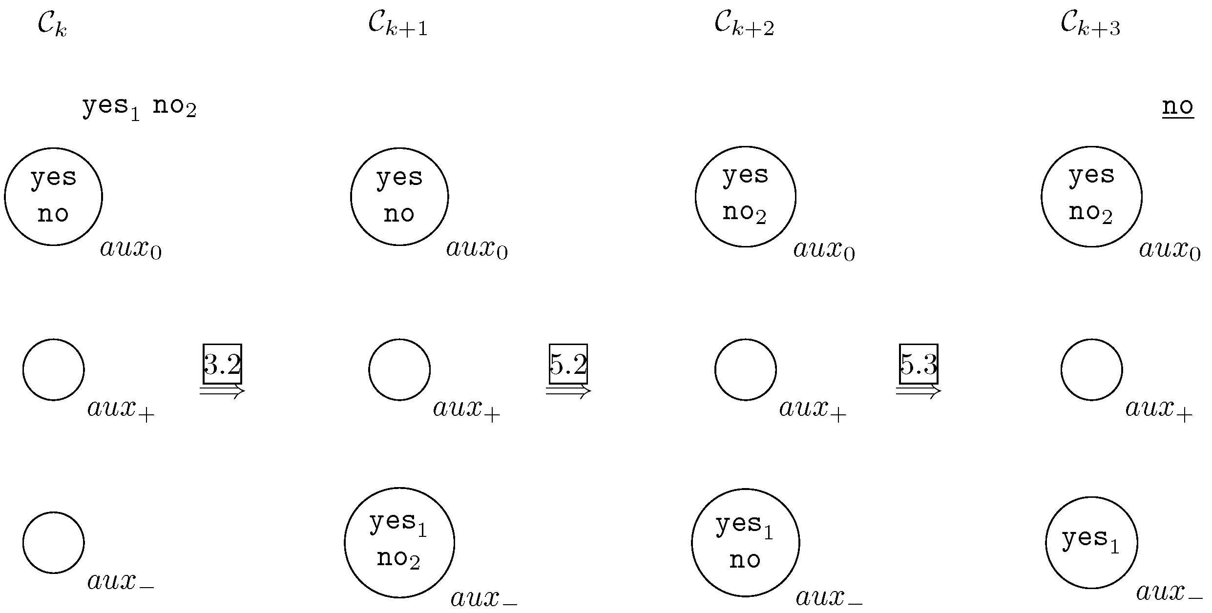
• Output stage
  The system $\mathrm{\Pi }\left(t\right)$ with input multiset $cod(u_1,u_2)$ sends the right answer to the environment according to the results obtained in the previous stage. Bearing in mind that rules 3.1, 3.2, 3.3 and 3.4 are cooperative, they will only be applicable when the environment receive the answers from ${\mathrm{\Pi }}^{\left(1\right)}\left(t_1\right)+co{d}_1\left(u_1\right)$ and ${\mathrm{\Pi }}^{\left(2\right)}\left(t_2\right)+co{d}_2\left(u_2\right)$. Let us assume that at instant k both answers reach the environment (obviously, k depends on the computations selected in the simulations and $k\le 1+n$).

  -

  Affirmative answer.

  In this case, the answers of ${\mathrm{\Pi }}^{\left(1\right)}\left(t_1\right)+co{d}_1\left(u_1\right)$ and ${\mathrm{\Pi }}^{\left(2\right)}\left(t_2\right)+co{d}_2\left(u_2\right)$ will be ${\mathtt{yes}}_1$ and ${\mathtt{yes}}_2$, respectively. By applying rule 3.1, objects ${\mathtt{yes}}_1$ and ${\mathtt{yes}}_2$ are sent to cell $au{x}_{+}$, that is ${\mathcal{C}}_{k+1}\left(au{x}_{+}\right)=\{{\mathtt{yes}}_1,{\mathtt{yes}}_2\}$. By applying rule 4.1 we will have ${\mathcal{C}}_{k+2}\left(au{x}_{+}\right)=\{\mathtt{yes},{\mathtt{yes}}_2\}$ and ${\mathcal{C}}_{k+2}\left(au{x}_0\right)=\{{\mathtt{yes}}_1,\mathtt{no}\}$. Finally, by applying rule 4.2 the system send out to the object yes and the system halts. It is graphically depicted in Figure 2.

  

  Figure 2. The answer of ${\mathrm{\Pi }}^{\left(1\right)}\left(t_1\right)$ is yes and the answer of ${\mathrm{\Pi }}^{\left(2\right)}\left(t_2\right)$ is yes.

  -

  Negative answer.

  In this case, at least one answer of ${\mathrm{\Pi }}^{\left(1\right)}\left(t_1\right)+co{d}_1\left(u_1\right)$ or ${\mathrm{\Pi }}^{\left(2\right)}\left(t_2\right)+co{d}_2\left(u_2\right)$ must be negative. By applying rule 3.2 or 3.3 or 3.4, cell $au{x}_{-}$ from configuration ${\mathcal{C}}_{k+1}$ will contain object ${\mathtt{no}}_1$ either object ${\mathtt{no}}_2$ either both of them. By applying rule 5.1 or rule 5.2 (only one of them because cell $au{x}_0$ from configuration ${\mathcal{C}}_{k+1}$ only contain one object no) will have $\mathtt{no}\in {\mathcal{C}}_{k+2}\left(au{x}_{-}\right)$. Finally, by applying rule 5.3 the system send out to the object no and the system halts. It is graphically depicted in Figure 3.

  

  Figure 3. The answer of ${\mathrm{\Pi }}^{\left(1\right)}\left(t_1\right)$ is yes and the answer of ${\mathrm{\Pi }}^{\left(2\right)}\left(t_2\right)$ is no.

Remark 1.

Concerning the proof of Theorem 1, we would like to draw attention to several aspects:

(a) 

Recognizer cooperative tissue-like membrane systems from class $\mathcal{R}$ are required to allow the use of communication rules with the length of at least 2, and the length of the new rules added is exactly 2.

(b) 

A explicit solution of the product problem product is provided from two respective solutions of the problems involved in that operation.

Corollary 1.

If $\mathcal{R}$ is a presumably efficient computing model of a recognizer tissue-like membrane system, thenDP ∪ co-DP$\subseteq {\mathbf{PMC}}_{\mathcal{R}}$.

Proof. 

First, let us note that if $\mathcal{R}$ is a presumably efficient computing model of a recognizer tissue-like membrane system and P ≠NP, then systems from $\mathcal{R}$ are cooperative (see [19,20] for details). Let X be an NP complete problem such that $X\in {\mathbf{PMC}}_{\mathcal{R}}$. Then, the complement problem $\overline{X}$ is a co-NP complete problem such that belongs to class ${\mathbf{PMC}}_{\mathcal{R}}$. From Theorem 1, we deduce that $X\otimes \overline{X}\in {\mathbf{PMC}}_{\mathcal{R}}$. Since the product problem $X\otimes \overline{X}$ is a DP complete problem and the complexity class ${\mathbf{PMC}}_{\mathcal{R}}$ is closed under complement and under polynomial-time reduction, DP ∪ co-DP $\subseteq {\mathbf{PMC}}_{\mathcal{R}}$ follows.    □

Remark 2.

According with the proofs of Theorem 1 and Corollary 1, a polynomial time and uniform solution to aDP-complete problem by means of a family of recognizer cooperative tissue-like membrane systems, can beexplicitly designedfrom a given polynomial time and uniform solution to aNP-complete problem. In fact, given anNP-complete problem X such that $X\in {\mathbf{PMC}}_{\mathcal{R}}$, where $\mathcal{R}$ is a class of presumably efficient computing model of a recognizer tissue-like membrane system, aDP-complete problem, the product problem $X\otimes \overline{X}$, is associated with it, in such a manner that if $X\in {\mathbf{PMC}}_{\mathcal{R}}$ then $X\otimes \overline{X}\in {\mathbf{PMC}}_{\mathcal{R}}$, for such kind class $\mathcal{R}$ of recognizer tissue-like systems.

3. Solving DP-Complete Problems by Using a New Methodology

In this section, the main Theorem is used to provide solutions to some DP-complete problems obtained from specific solutions to NP-complete problems in the framework of recognizer cooperative tissue-like membrane systems. In particular we use the efficient solution to the SAT problem by means of a family of recognizer tissue P systems with symport/antiport rules with length at most 2 and division rules from [23], that is based on the classical generation-checking-output workflow. As mentioned in the methodology, given a family of recognizer P systems ${\mathbf{\Pi }}^{\left(\mathbf{1}\right)}$ from $\mathcal{R}$ efficiently solving a problem X from the complexity class $\mathbf{C}$, then a family of recognizer P systems ${\mathbf{\Pi }}^{\left(\mathbf{2}\right)}$ from $\mathcal{R}$ that solves the complementary problem of X, being $\overline{X}\in \mathbf{co}-\mathbf{C}$.

The SAT-UNSAT problem is defined as follows: Let ${\phi }_1$ (respectively, ${\phi }_2$) be a propositional logic formula with $n_1$ variables (resp., $n_2$ variables) and $p_1$ clauses (resp., $p_2$ clauses). We say that the pair $({\phi }_1,{\phi }_2)$ is true if and only if ${\phi }_1$ is satisfiable and ${\phi }_2$ is unsatisfiable. Formally, let $\mathtt{SAT}-\mathtt{UNSAT}=(I_{\mathtt{SAT}-\mathtt{UNSAT}},{\theta }_{\mathtt{SAT}-\mathtt{UNSAT}})$, where $I_{\mathtt{SAT}-\mathtt{UNSAT}}=\{({\phi }_i,{\phi }_2)\mid {\phi }_1,{\phi }_2\mathrm{are}\mathrm{propositional}\mathrm{logic}\mathrm{formulae}\mathrm{in}\mathrm{CNF}$ $\mathrm{and}\mathrm{in}\mathrm{a}\mathrm{simplified}\mathrm{form}\}$.

$${\theta }_{\mathtt{SAT}-\mathtt{UNSAT}}\left(({\phi }_1,{\phi }_2)\right)=\left\{\begin{array}{c}1\mathit{iff}{\phi }_1\in L_{\mathtt{SAT}}\wedge {\phi }_2\in L_{\mathtt{UNSAT}}\hfill \\ 0otherwise\hfill \end{array}\right.$$

Let ${\mathrm{\Gamma }}^{\left(1\right)}$ be the working alphabet of ${\mathbf{\Pi }}^{\left(\mathbf{1}\right)}$ and ${\mathrm{\Gamma }}^{\left(2\right)}$ be the working alphabet of ${\mathbf{\Pi }}^{\left(\mathbf{2}\right)}$. Given that we need that ${\mathrm{\Gamma }}^{\left(1\right)}\cap {\mathrm{\Gamma }}^{\left(2\right)}=\varnothing$, we let ${\mathrm{\Gamma }}^{\left(2\right)}=\{\mathbf{a}\mid a\in {\mathrm{\Gamma }}^{\left(1\right)}\}$; that is, objects from ${\mathrm{\Gamma }}^{\left(2\right)}$ will be boldfaced versions of objects from ${\mathrm{\Gamma }}^{\left(1\right)}$. In ${\mathrm{\Gamma }}^{\left(1\right)}$ (respectively, ${\mathrm{\Gamma }}^{\left(2\right)}$) we will change objects $\mathtt{yes}$ and $\mathtt{no}$ by objects ${\mathtt{yes}}_1$ and ${\mathtt{no}}_1$ (resp., ${\mathtt{yes}}_2$ and ${\mathtt{no}}_2$). In addition, let $H^{\left(1\right)}$ be the working alphabet of ${\mathbf{\Pi }}^{\left(\mathbf{1}\right)}$. The set of labels $H^{\left(2\right)}$ of ${\mathbf{\Pi }}^{\left(\mathbf{2}\right)}$ will be defined as $H^{\left(2\right)}=\{\mathbf{h}\mid h\in H^{\left(1\right)}\}$. For each quadruple of natural numbers $n_1,p_1,n_2,p_2\in \mathbb{N}$, we will consider the recognizer tissue P system with cell division and symport/antiport rules of length at most 2.

$$\begin{array}{c}\mathrm{\Pi }\left(⟨⟨n_1,p_1⟩,⟨n_2,p_2⟩⟩\right)=(\mathrm{\Gamma },\mathcal{E},\Sigma ,{\mathcal{M}}_1,\dots ,{\mathcal{M}}_{n_1{p}_1+3},{\mathcal{M}}_{\mathbf{1}},\dots ,{\mathcal{M}}_{{\mathbf{n}}_{\mathbf{2}}{\mathbf{p}}_{\mathbf{2}}+\mathbf{3}},{\mathcal{M}}_{au{x}_{+}},\\ {\mathcal{M}}_{au{x}_{-}},{\mathcal{M}}_{au{x}_0},\mathcal{R},i_{in},i_{out})\end{array}$$

of degree $n_1{p}_1{\mathbf{n}}_{\mathbf{2}}{\mathbf{p}}_{\mathbf{2}}+6$ defined as follows:

(a)

$$\begin{array}{ccc}\mathrm{\Gamma }\hfill & =\hfill & {\mathrm{\Gamma }}^{\prime }\cup \{a^{\prime }\mid a\in {\mathrm{\Gamma }}^{\prime }\},\hfill \\ {\mathrm{\Gamma }}^{\prime }\hfill & =\hfill & \Sigma \cup \mathcal{E}\cup \{\mathtt{yes},\mathtt{no}\}\cup \{{\mathtt{yes}}_1,{\mathtt{no}}_1,\alpha ,{\beta }_0,{\gamma }_0\}\cup \{c_j\mid 1\le k\le p_1\}\cup \hfill \\ \hfill & & \{{\alpha }_k\mid 0\le k\le n_1{p}_1-1\}\cup \{a_{i,j}\mid 1\le i\le n_1,1\le j\le p_1\}\cup \hfill \\ \hfill & & \{T_{i,j},F_{i,j}\mid 1\le i\le n_1,1\le j\le p_1\}\cup \hfill \\ \hfill & & \{x_{i,j,k},{\overline{x}}_{i,j,k}\mid 1\le i\le n_1,1\le j\le p_1,0\le k\le n_1{p}_1\}\cup \hfill \\ & & \{{\mathtt{yes}}_2,{\mathtt{no}}_2,\mathbf{ff},{\mathbf{fi}}_{\mathbf{0}},{\mathbf{fl}}_{\mathbf{0}}\}\cup \{{\mathbf{c}}_{\mathbf{j}}\mid 1\le k\le p_2\}\cup \hfill \\ \hfill & & \{{\mathbf{ff}}_{\mathbf{k}}\mid 0\le k\le n_2{p}_2-1\}\cup \{{\mathbf{a}}_{\mathbf{i},\mathbf{j}}\mid 1\le i\le n_2,1\le j\le p_2\}\cup \hfill \\ \hfill & & \{{\mathbf{T}}_{\mathbf{i},\mathbf{j}},{\mathbf{F}}_{\mathbf{i},\mathbf{j}}\mid 1\le i\le n_2,1\le j\le p_2\}\cup \hfill \\ \hfill & & \{{\mathbf{x}}_{\mathbf{i},\mathbf{j},\mathbf{k}},{\overline{\mathbf{x}}}_{\mathbf{i},\mathbf{j},\mathbf{k}}\mid 1\le i\le n_2,1\le j\le p_2,0\le k\le n_2{p}_2\}\hfill \end{array}$$

(b)

$$\begin{array}{ccc}\mathcal{E}\hfill & =\hfill & \{{\alpha }_k\mid n_1{p}_1\le k\le 2n_1{p}_1+2\}\cup \{{\beta }_k\mid 1\le k\le 2n_1{p}_1+4\}\cup \hfill \\ \hfill & & \{{\gamma }_k\mid 1\le k\le 2n_1{p}_1+5\}\cup \hfill \\ & & \{x_{i,j,k},{\overline{x}}_{i,j,k}\mid 1\le i\le n_1,1\le j\le p_1,n_1{p}_1+1\le k\le 2n_1{p}_1\}\cup \hfill \\ & & \{{\mathbf{ff}}_{\mathbf{k}}\mid n_2{p}_2\le k\le 2n_2{p}_2+2\}\cup \{{\mathbf{fi}}_{\mathbf{k}}\mid 1\le k\le 2n_2{p}_2+4\}\cup \hfill \\ \hfill & & \{{\mathbf{fl}}_{\mathbf{k}}\mid 1\le k\le 2n_2{p}_2+5\}\cup \hfill \\ & & \{{\mathbf{x}}_{\mathbf{i},\mathbf{j},\mathbf{k}},{\overline{\mathbf{x}}}_{\mathbf{i},\mathbf{j},\mathbf{k}}\mid 1\le i\le n_2,1\le j\le p_2,n_2{p}_2+1\le k\le 2n_2{p}_2\}\hfill \end{array}$$

(c)

$$\begin{array}{ccc}\Sigma \hfill & =\hfill & \{x_{i,j,0},{\overline{x}}_{i,j,0}\mid 1\le i\le n_1,1\le j\le p_1\}\cup \hfill \\ & & \{{\mathbf{x}}_{\mathbf{i},\mathbf{j},\mathbf{0}},{\overline{\mathbf{x}}}_{\mathbf{i},\mathbf{j},\mathbf{0}}\mid 1\le i\le n_2,1\le j\le p_2\}\hfill \end{array}$$

(d)

${\mathcal{M}}_i=\varnothing$ for $i\in \{au{x}_{+},au{x}_{-}\}$, ${\mathcal{M}}_{au{x}_0}=\{{\beta }_0^{*},{\gamma }_0^{*}\}\cup$ $\{a_{i,j}^{*}\mid 1\le i\le n_1,1\le j\le p_1\}\cup \{c_j^{*}\mid 1\le j\le p_1\}\cup \left\{{\alpha }^{*}\right\}\cup$ $\left\{{\alpha }_0^{*}\right\}\cup \{{\mathbf{fi}}_{\mathbf{0}},{\mathbf{fl}}_{\mathbf{0}}\}\cup$ $\{{\mathbf{a}}_{\mathbf{i},\mathbf{j}}\mid 1\le i\le n_2,1\le j\le p_2\}\cup \{{\mathbf{c}}_{\mathbf{j}}\mid 1\le j\le p_2\}\cup \left\{\mathbf{ff}\right\}\cup$ $\left\{{\mathbf{ff}}_{\mathbf{0}}\right\}\cup$ $\{{\mathtt{yes}}_1,{\mathtt{no}}_1,{\beta }_0^{*},{\gamma }_0^{*}\}\cup$ $\{a_{i,j}^{*}\mid 1\le i\le n_1,1\le j\le p_1\}\cup \{c_j^{*}\mid 1\le j\le p_1\}\cup \left\{{\alpha }^{*}\right\}\cup$ $\left\{{\alpha }_0^{*}\right\}\cup \{{\mathtt{yes}}_2,{\mathtt{no}}_2,{\mathbf{fi}}_{\mathbf{0}}^{*},{\mathbf{fl}}_{\mathbf{0}}^{*}\}\cup$ $\{{\mathbf{a}}_{\mathbf{i},\mathbf{j}}^{\mathbf{*}}\mid 1\le i\le n_2,1\le j\le p_2\}\cup \{{\mathbf{c}}_{\mathbf{j}}^{*}\mid 1\le j\le p_2\}\cup \left\{{\mathbf{ff}}^{\mathbf{*}}\right\}\cup$ $\left\{{\mathbf{ff}}_{\mathbf{0}}^{\mathbf{*}}\right\},{\mathcal{M}}_i=\{a^{\prime }\mid a\in {\mathcal{M}}_i\mathrm{in}\mathrm{the}\mathrm{original}\mathrm{solution}\},{\mathcal{M}}_{\mathbf{i}}=\{{\mathbf{a}}^{\prime }\mid a\in {\mathcal{M}}_i\mathrm{in}\mathrm{the}\mathrm{original}\mathrm{solution}\}$

(e)

The set of rules $\mathcal{R}$ is the following:

$\left.\begin{array}{c}{\left[a_{i,j}\right]}_{n_1{p}_1+2}\to {\left[T_{i,j}\right]}_{n_1{p}_1+2}{\left[F_{i,j}\right]}_{n_1{p}_1+2}\hfill \\ (n_1{p}_1+2,T_{i,j}{F}_{i,j^{\prime }},/\lambda ,env)\hfill \end{array}\right\}for\begin{array}{c}1\le i\le n_1,1\le j,j^{\prime }\le p_1\hfill \end{array}$

$\left.\begin{array}{c}(n_1{p}_1+1,x_{i,j,0}/\lambda ,i+n_1·(j-1))\hfill \\ (n_1{p}_1+1,{\overline{x}}_{i,j,0}/\lambda ,i+n_1·(j-1))\hfill \end{array}\right\}for\begin{array}{c}1\le i\le n_1,\hfill \\ 1\le j\le p_1\hfill \end{array}$

$\left.\begin{array}{c}{\left[x_{i,j,k}\right]}_{i+n_1·(j-1)}\to {\left[x_{i,j,k+1}\right]}_{i+n_1·(j-1)}{\left[x_{i,j,k+1}\right]}_{i+n_1·(j-1)}\hfill \\ {\left[{\overline{x}}_{i,j,k}\right]}_{i+n_1·(j-1)}\to {\left[{\overline{x}}_{i,j,k+1}\right]}_{i+n_1·(j-1)}{\left[{\overline{x}}_{i,j,k+1}\right]}_{i+n_1·(j-1)}\hfill \end{array}\right\}for\begin{array}{c}1\le i\le n_1,\hfill \\ 1\le j\le p_1,\hfill \\ 0\le k\le n_1{p}_1-1\hfill \end{array}$

$\left.\begin{array}{c}(i+n_1·(j-1),x_{i,j,k}/x_{i,j,k+1},env)\hfill \\ (i+n_1·(j-1),{\overline{x}}_{i,j,k}/{\overline{x}}_{i,j,k+1},env)\hfill \end{array}\right\}for\begin{array}{c}1\le i\le n_1,\hfill \\ 1\le j\le p_1,\hfill \\ n_1{p}_1\le k\le 2n_1{p}_1-1\hfill \end{array}$

$\left.\begin{array}{c}(n_1{p}_1+2,T_{i,j}/x_{i,j,2n_1{p}_1},i+n_1·(j-1))\hfill \\ (n_1{p}_1+2,F_{i,j}/{\overline{x}}_{i,j,2n_1{p}_1},i+n_1·(j-1))\hfill \end{array}\right\}for\begin{array}{c}1\le i\le n_1,\hfill \\ 1\le j\le p_1\hfill \end{array}$

$\left.\begin{array}{c}(n_1{p}_1+2,c_j{x}_{i,j,2n_1{p}_1}/\lambda ,env)\hfill \\ (n_1{p}_1+2,c_j{\overline{x}}_{i,j,2n_1{p}_1}/\lambda ,env)\hfill \end{array}\right\}for\begin{array}{c}1\le i\le n_1,1\le j\le p_1\hfill \end{array}$

$\left.\begin{array}{c}{\left[{\alpha }_k\right]}_{n_1{p}_1+3}\to {\left[{\alpha }_{k+1}\right]}_{n_1{p}_1+3}{\left[{\alpha }_{k+1}\right]}_{n_1{p}_1+3}\hfill \end{array}\right\}for\begin{array}{c}0\le k\le n_1{p}_1-1\hfill \end{array}$

$\begin{array}{c}(n_1{p}_1+3,{\alpha }_{n_1{p}_1+k}/{\alpha }_{n_1{p}_1+k+1},env)\hfill \end{array}for\begin{array}{c}0\le k\le n_1{p}_1+1\hfill \end{array}$

$\begin{array}{c}(n_1{p}_1+1,{\beta }_k/{\beta }_{k+1},env)\hfill \end{array}for\begin{array}{c}0\le k\le 2n_1{p}_1+3\hfill \end{array}$

$\begin{array}{c}(n_1{p}_1+1,{\gamma }_k/{\gamma }_{k+1},env)\hfill \end{array}for\begin{array}{c}0\le k\le 2n_1{p}_1+4\hfill \end{array}$

$\begin{array}{c}(n_1{p}_1+2,\alpha /{\alpha }_{2n_1{p}_1+2},n_1{p}_1+3)\hfill \end{array}$

$\begin{array}{c}(n_1{p}_1+2,{\alpha }_{2n_1{p}_1+2}{c}_j/\lambda ,env)\hfill \end{array}for\begin{array}{c}1\le j\le p_1\hfill \end{array}$

$(n_1{p}_1+1,{\beta }_{2n_1{p}_1+4},{\gamma }_{2n_1{p}_1+5}/\lambda ,n_1{p}_1+3)$

$(n_1{p}_1+1,{\mathtt{no}}_1/{\beta }_{2n_1{p}_1+4},n_1{p}_1+3)$

$(n_1{p}_1+3,{\mathtt{no}}_1/\lambda ,env)$

$(n_1{p}_1+1,{\beta }_{2n_1{p}_1+4}/{\alpha }_{2n_1{p}_1+2},n_1{p}_1+2)$

$(n_1{p}_1+1,{\alpha }_{2n_1{p}_1+2}{\mathtt{yes}}_1/\lambda ,env)$

$\left.\begin{array}{c}{\left[{\mathbf{a}}_{\mathbf{i},\mathbf{j}}\right]}_{{\mathbf{n}}_{\mathbf{2}}{\mathbf{p}}_{\mathbf{2}}+\mathbf{2}}\to {\left[{\mathbf{T}}_{\mathbf{i},\mathbf{j}}\right]}_{{\mathbf{n}}_{\mathbf{2}}{\mathbf{p}}_{\mathbf{2}}+\mathbf{2}}{\left[{\mathbf{F}}_{\mathbf{i},\mathbf{j}}\right]}_{{\mathbf{n}}_{\mathbf{2}}{\mathbf{p}}_{\mathbf{2}}+\mathbf{2}}\hfill \\ ({\mathbf{n}}_{\mathbf{2}}{\mathbf{p}}_{\mathbf{2}}+\mathbf{2},{\mathbf{T}}_{\mathbf{i},\mathbf{j}}{\mathbf{F}}_{\mathbf{i},{\mathbf{j}}^{\prime }},/\lambda ,env)\hfill \end{array}\right\}for\begin{array}{c}1\le \mathbf{i}\le {\mathbf{n}}_{\mathbf{2}},1\le \mathbf{j},{\mathbf{j}}^{\prime }\le {\mathbf{p}}_{\mathbf{2}}\hfill \end{array}$

$\left.\begin{array}{c}({\mathbf{n}}_{\mathbf{2}}{\mathbf{p}}_{\mathbf{2}}+\mathbf{1},{\mathbf{x}}_{\mathbf{i},\mathbf{j},\mathbf{0}}/\lambda ,\mathbf{i}+{\mathbf{n}}_{\mathbf{2}}·(\mathbf{j}-\mathbf{1}))\hfill \\ ({\mathbf{n}}_{\mathbf{2}}{\mathbf{p}}_{\mathbf{2}}+\mathbf{1},{\overline{\mathbf{x}}}_{\mathbf{i},\mathbf{j},\mathbf{0}}/\lambda ,\mathbf{i}+{\mathbf{n}}_{\mathbf{2}}·(\mathbf{j}-\mathbf{1}))\hfill \end{array}\right\}for\begin{array}{c}1\le \mathbf{i}\le {\mathbf{n}}_{\mathbf{2}},\hfill \\ 1\le \mathbf{j}\le {\mathbf{p}}_{\mathbf{2}}\hfill \end{array}$

$\left.\begin{array}{c}{\left[{\mathbf{x}}_{\mathbf{i},\mathbf{j},\mathbf{k}}\right]}_{\mathbf{i}+{\mathbf{n}}_{\mathbf{2}}·(\mathbf{j}-\mathbf{1})}\to {\left[{\mathbf{x}}_{\mathbf{i},\mathbf{j},\mathbf{k}+\mathbf{1}}\right]}_{\mathbf{i}+{\mathbf{n}}_{\mathbf{2}}·(\mathbf{j}-\mathbf{1})}{\left[{\mathbf{x}}_{\mathbf{i},\mathbf{j},\mathbf{k}+\mathbf{1}}\right]}_{\mathbf{i}+{\mathbf{n}}_{\mathbf{2}}·(\mathbf{j}-\mathbf{1})}\hfill \\ {\left[{\overline{\mathbf{x}}}_{\mathbf{i},\mathbf{j},\mathbf{k}}\right]}_{\mathbf{i}+{\mathbf{n}}_{\mathbf{2}}·(\mathbf{j}-\mathbf{1})}\to {\left[{\overline{\mathbf{x}}}_{\mathbf{i},\mathbf{j},\mathbf{k}+\mathbf{1}}\right]}_{\mathbf{i}+{\mathbf{n}}_{\mathbf{2}}·(\mathbf{j}-\mathbf{1})}{\left[{\overline{\mathbf{x}}}_{\mathbf{i},\mathbf{j},\mathbf{k}+\mathbf{1}}\right]}_{\mathbf{i}+{\mathbf{n}}_{\mathbf{2}}·(\mathbf{j}-\mathbf{1})}\hfill \end{array}\right\}for\begin{array}{c}1\le \mathbf{i}\le {\mathbf{n}}_{\mathbf{2}},\hfill \\ 1\le \mathbf{j}\le {\mathbf{p}}_{\mathbf{2}},\hfill \\ 0\le \mathbf{k}\le {\mathbf{n}}_{\mathbf{2}}{\mathbf{p}}_{\mathbf{2}}-1\hfill \end{array}$

$\left.\begin{array}{c}(\mathbf{i}+{\mathbf{n}}_{\mathbf{2}}·(\mathbf{j}-\mathbf{1}),{\mathbf{x}}_{\mathbf{i},\mathbf{j},\mathbf{k}}/{\mathbf{x}}_{\mathbf{i},\mathbf{j},\mathbf{k}+\mathbf{1}},env)\hfill \\ (\mathbf{i}+{\mathbf{n}}_{\mathbf{2}}·(\mathbf{j}-\mathbf{1}),{\overline{\mathbf{x}}}_{\mathbf{i},\mathbf{j},\mathbf{k}}/{\overline{\mathbf{x}}}_{\mathbf{i},\mathbf{j},\mathbf{k}+\mathbf{1}},env)\hfill \end{array}\right\}for\begin{array}{c}1\le \mathbf{i}\le {\mathbf{n}}_{\mathbf{2}},\hfill \\ 1\le \mathbf{j}\le {\mathbf{p}}_{\mathbf{2}},\hfill \\ {\mathbf{n}}_{\mathbf{2}}{\mathbf{p}}_{\mathbf{2}}\le \mathbf{k}\le 2{\mathbf{n}}_{\mathbf{2}}{\mathbf{p}}_{\mathbf{2}}-1\hfill \end{array}$

$\left.\begin{array}{c}({\mathbf{n}}_{\mathbf{2}}{\mathbf{p}}_{\mathbf{2}}+\mathbf{2},{\mathbf{T}}_{\mathbf{i},\mathbf{j}}/{\mathbf{x}}_{\mathbf{i},\mathbf{j},\mathbf{2}{\mathbf{n}}_{\mathbf{2}}{\mathbf{p}}_{\mathbf{2}}},\mathbf{i}+{\mathbf{n}}_{\mathbf{2}}·(\mathbf{j}-\mathbf{1}))\hfill \\ ({\mathbf{n}}_{\mathbf{2}}{\mathbf{p}}_{\mathbf{2}}+\mathbf{2},{\mathbf{F}}_{\mathbf{i},\mathbf{j}}/{\overline{\mathbf{x}}}_{\mathbf{i},\mathbf{j},\mathbf{2}{\mathbf{n}}_{\mathbf{2}}{\mathbf{p}}_{\mathbf{2}}},\mathbf{i}+{\mathbf{n}}_{\mathbf{2}}·(\mathbf{j}-\mathbf{1}))\hfill \end{array}\right\}for\begin{array}{c}1\le \mathbf{i}\le {\mathbf{n}}_{\mathbf{2}},\hfill \\ 1\le \mathbf{j}\le {\mathbf{p}}_{\mathbf{2}}\hfill \end{array}$

$\left.\begin{array}{c}({\mathbf{n}}_{\mathbf{2}}{\mathbf{p}}_{\mathbf{2}}+\mathbf{2},{\mathbf{c}}_{\mathbf{j}}{\mathbf{x}}_{\mathbf{i},\mathbf{j},\mathbf{2}{\mathbf{n}}_{\mathbf{2}}{\mathbf{p}}_{\mathbf{2}}}/\lambda ,env)\hfill \\ ({\mathbf{n}}_{\mathbf{2}}{\mathbf{p}}_{\mathbf{2}}+\mathbf{2},{\mathbf{c}}_{\mathbf{j}}{\overline{\mathbf{x}}}_{\mathbf{i},\mathbf{j},\mathbf{2}{\mathbf{n}}_{\mathbf{2}}{\mathbf{p}}_{\mathbf{2}}}/\lambda ,env)\hfill \end{array}\right\}for\begin{array}{c}1\le \mathbf{i}\le {\mathbf{n}}_{\mathbf{2}},1\le \mathbf{j}\le {\mathbf{p}}_{\mathbf{2}}\hfill \end{array}$

$\left.\begin{array}{c}{\left[{\mathbf{ff}}_{\mathbf{k}}\right]}_{{\mathbf{n}}_{\mathbf{2}}{\mathbf{p}}_{\mathbf{2}}+\mathbf{3}}\to {\left[{\mathbf{ff}}_{\mathbf{k}+\mathbf{1}}\right]}_{{\mathbf{n}}_{\mathbf{2}}{\mathbf{p}}_{\mathbf{2}}+\mathbf{3}}{\left[{\mathbf{ff}}_{\mathbf{k}+\mathbf{1}}\right]}_{{\mathbf{n}}_{\mathbf{2}}{\mathbf{p}}_{\mathbf{2}}+\mathbf{3}}\hfill \end{array}\right\}for\begin{array}{c}0\le \mathbf{k}\le {\mathbf{n}}_{\mathbf{2}}{\mathbf{p}}_{\mathbf{2}}-1\hfill \end{array}$

$\begin{array}{c}({\mathbf{n}}_{\mathbf{2}}{\mathbf{p}}_{\mathbf{2}}+\mathbf{3},{\mathbf{ff}}_{{\mathbf{n}}_{\mathbf{2}}{\mathbf{p}}_{\mathbf{2}}+\mathbf{k}}/{\mathbf{ff}}_{{\mathbf{n}}_{\mathbf{2}}{\mathbf{p}}_{\mathbf{2}}+\mathbf{k}+\mathbf{1}},env)\hfill \end{array}for\begin{array}{c}0\le \mathbf{k}\le {\mathbf{n}}_{\mathbf{2}}{\mathbf{p}}_{\mathbf{2}}+1\hfill \end{array}$

$\begin{array}{c}(\mathbf{np}+\mathbf{1},{\mathbf{fi}}_{\mathbf{k}}/{\mathbf{fi}}_{\mathbf{k}+\mathbf{1}},env)\hfill \end{array}for\begin{array}{c}0\le \mathbf{k}\le 2{\mathbf{n}}_{\mathbf{2}}{\mathbf{p}}_{\mathbf{2}}+3\hfill \end{array}$

$\begin{array}{c}({\mathbf{n}}_{\mathbf{2}}{\mathbf{p}}_{\mathbf{2}}+\mathbf{1},{\mathbf{fl}}_{\mathbf{k}}/{\mathbf{fl}}_{\mathbf{k}+\mathbf{1}},env)\hfill \end{array}for\begin{array}{c}0\le \mathbf{k}\le 2{\mathbf{n}}_{\mathbf{2}}{\mathbf{p}}_{\mathbf{2}}+4\hfill \end{array}$

$\begin{array}{c}({\mathbf{n}}_{\mathbf{2}}{\mathbf{p}}_{\mathbf{2}}+\mathbf{2},\mathbf{ff}/{\mathbf{ff}}_{\mathbf{2}{\mathbf{n}}_{\mathbf{2}}{\mathbf{p}}_{\mathbf{2}}+\mathbf{2}},{\mathbf{n}}_{\mathbf{2}}{\mathbf{p}}_{\mathbf{2}}+\mathbf{3})\hfill \end{array}$

$\begin{array}{c}({\mathbf{n}}_{\mathbf{2}}{\mathbf{p}}_{\mathbf{2}}+\mathbf{2},{\mathbf{ff}}_{\mathbf{2}{\mathbf{n}}_{\mathbf{2}}{\mathbf{p}}_{\mathbf{2}}+\mathbf{2}}{\mathbf{c}}_{\mathbf{j}}/\lambda ,env)\hfill \end{array}for\begin{array}{c}1\le \mathbf{j}\le {\mathbf{p}}_{\mathbf{2}}\hfill \end{array}$

$({\mathbf{n}}_{\mathbf{2}}{\mathbf{p}}_{\mathbf{2}}+\mathbf{1},{\mathbf{fi}}_{\mathbf{2}{\mathbf{n}}_{\mathbf{2}}{\mathbf{p}}_{\mathbf{2}}+\mathbf{4}},{\mathbf{fl}}_{\mathbf{2}{\mathbf{n}}_{\mathbf{2}}{\mathbf{p}}_{\mathbf{2}}+\mathbf{5}}/\lambda ,{\mathbf{n}}_{\mathbf{2}}{\mathbf{p}}_{\mathbf{2}}+\mathbf{3})$

$({\mathbf{n}}_{\mathbf{2}}{\mathbf{p}}_{\mathbf{2}}+\mathbf{1},{\mathtt{yes}}_2/{\mathbf{fi}}_{\mathbf{2}{\mathbf{n}}_{\mathbf{2}}{\mathbf{p}}_{\mathbf{2}}+\mathbf{4}},{\mathbf{n}}_{\mathbf{2}}{\mathbf{p}}_{\mathbf{2}}+\mathbf{3})$

$({\mathbf{n}}_{\mathbf{2}}{\mathbf{p}}_{\mathbf{2}}+\mathbf{3},{\mathtt{yes}}_2/\lambda ,env)$

$({\mathbf{n}}_{\mathbf{2}}{\mathbf{p}}_{\mathbf{2}}+\mathbf{1},{\mathbf{fi}}_{\mathbf{2}{\mathbf{n}}_{\mathbf{2}}{\mathbf{p}}_{\mathbf{2}}+\mathbf{4}}/{\mathbf{ff}}_{\mathbf{2}{\mathbf{n}}_{\mathbf{2}}{\mathbf{p}}_{\mathbf{2}}+\mathbf{2}},{\mathbf{n}}_{\mathbf{2}}{\mathbf{p}}_{\mathbf{2}}+\mathbf{2})$

$({\mathbf{n}}_{\mathbf{2}}{\mathbf{p}}_{\mathbf{2}}+\mathbf{1},{\mathbf{ff}}_{\mathbf{2}{\mathbf{n}}_{\mathbf{2}}{\mathbf{p}}_{\mathbf{2}}+\mathbf{2}}{\mathtt{no}}_2/\lambda ,env)$

Apart from these, all rules indicated in Section 2 must be added.

(f)

$i_{in}=au{x}_0$ and $i_{out}=env$

For details about the behavior of the original SAT solution, we refer the reader to [23].

4. Insights from the Evolution of the System

We recall that non-bold indexes and objects correspond to the indexes and objects from the solution to SAT and bold indexes and objects correspond to the indexes and objects from the solution to UNSAT. Figure 4 and Figure 5 show the evolution of the number of cells labeled by $i+n_1·(j-1),n_1{p}_1+2$ and $n_1{p}_1+3$ (respectively, $\mathbf{i}+{\mathbf{n}}_{\mathbf{2}}·(\mathbf{j}-\mathbf{1}),{\mathbf{n}}_{\mathbf{2}}{\mathbf{p}}_{\mathbf{2}}+\mathbf{2}$ and ${\mathbf{n}}_{\mathbf{2}}{\mathbf{p}}_{\mathbf{2}}+\mathbf{3}$). First of all, it can be observed that the execution of division rules of cells labeled by $n_1{p}_1+2,n_1{p}_1+3,{\mathbf{n}}_{\mathbf{2}}{\mathbf{p}}_{\mathbf{2}}+\mathbf{2}$ and ${\mathbf{n}}_{\mathbf{2}}{\mathbf{p}}_{\mathbf{2}}+\mathbf{3}$ start in the second computational step, since the first one is reserved to the movements of objects from the cell $au{x}_0$ to their corresponding cell. In addition, since in the original solution the division of membranes labeled by $i+n_1·(j-1)$ and $\mathbf{i}+{\mathbf{n}}_{\mathbf{2}}·(\mathbf{j}-\mathbf{1})$ start at step 2, they start to be simulated at step 3 in $\mathrm{\Pi }\left(⟨u_1,u_2⟩\right)+cod\left((u_1,u_2)\right)$.

Figure 4. Evolution of the number of membranes of the $\mathtt{SAT}$ solution.

Figure 5. Evolution of membranes of the $\mathtt{UNSAT}$ solution.

Since division rules of cells labeled by $n_1{p}_1+2$ and ${\mathbf{n}}_{\mathbf{2}}{\mathbf{p}}_{\mathbf{2}}+\mathbf{2}$ can be non-consecutive due to the application of rules $(n_1{p}_1+2,T_{i,j}{F}_{i,j^{\prime }},/\lambda ,env)$ and $({\mathbf{n}}_{\mathbf{2}}{\mathbf{p}}_{\mathbf{2}}+\mathbf{2},{\mathbf{T}}_{\mathbf{i},\mathbf{j}}{\mathbf{F}}_{\mathbf{i},{\mathbf{j}}^{\prime }},/\lambda ,env)$, the number of membranes labeled by $n_1{p}_1+2$ and ${\mathbf{n}}_{\mathbf{2}}{\mathbf{p}}_{\mathbf{2}}+\mathbf{2}$ in configuration $1+k$ can be different to $2^k$.

The original solution takes $2np+8$ steps in the negative case and $2np+6$ in the case that there exists a truth assignment that makes true the input formula $\phi$, being n the number of variables and p the number of clauses. In Figure 6, we can see that the number of steps taken in the computation of $\mathrm{\Pi }\left(⟨u_1,u_2⟩\right)+cod\left((u_1,u_2)\right)$ depends on the number of steps of the original computation. In this case, $c_1<c_2$. In the figure, $m=max(c_1,c_2)+4$, being $c_i$ the computation time of ${\mathrm{\Pi }}^{\left(i\right)}\left(t_i\right)$, taking into account that it takes one step for the objects to prepare both ${\mathrm{\Pi }}^{\left(1\right)}\left(t_1\right)$ and ${\mathrm{\Pi }}^{\left(2\right)}\left(t_2\right)$ and three steps for the output stage. The cyan (first element in legend) line lies below the red (fourth element in legend) line until $n_1{p}_1+2$ and below the green (third element in legend) line from that point.

Figure 6. Global evolution of the number of membranes of the $\mathtt{SAT}-\mathtt{UNSAT}$ solution.

5. Conclusions

Considering $\mathcal{R}$ as a presumed efficient computing model of recognizer tissue-like membrane systems, meaning it possesses the capability to solve NP-complete problems in polynomial time, the time complexity class ${\mathbf{PMC}}_{\mathcal{R}}$ encompasses the complexity classes NP and co-NP [9]. In this paper, we enhance this finding by presenting a specific protocol for converting a solution of an NP-complete problem into a solution for a DP-complete problem. Here, DP represents the set of languages that can be expressed as the difference between two languages in NP or, equivalently, as the intersection of a language in NP and a language in co-NP. Thus, the following result has been obtained: $\mathbf{DP}\cup$ co-DP $\subseteq {\mathbf{PMC}}_{\mathcal{R}}$ In fact, a more general result has been obtained: let $X_1$ and $X_2$ be two decision problems in the class ${\mathbf{PMC}}_{\mathcal{R}}$, being $\mathcal{R}$ a class of recognizer cooperative tissue P systems. Then, the problem $X_1\otimes X_2$ belongs also to the class ${\mathbf{PMC}}_{\mathcal{R}}$. The protocol to transform the solutions to $X_1$ and $X_2$ to a solution to the problem $X_1\otimes X_2$ takes only four extra steps with respect to the maximum number of steps of the solutions of $X_1$ and $X_2$, thus making it an efficient way to transform the solutions. Of course, this methodology cannot be applied if the tissue P systems are non-cooperative, because some objects need this behavior to move from one region to another region, this making it impossible to implement this collaboration between objects.

In [15], the authors provided an exact characterization of the class ${\mathbf{PMC}}_{\mathcal{TFC}}$, which is even more challenging than the result presented in this study. However, it is important to consider two key factors. Firstly, the definition of recognizer membrane systems in [15] differs from the definition given in [9]. Secondly, the strength of this paper lies not only in the lower bound but also in the automatic protocol provided for transforming a solution of a $\mathbf{NP}$-complete problem into a $\mathbf{DP}$-complete problem. This protocol can be readily implemented and simulated using software simulators like P-Lingua, designed specifically for membrane systems.

In [10], the authors introduced a similar methodology for transforming a solution of a $\mathbf{NP}$-complete problem into a solution of a $\mathbf{DP}$-complete problem within the framework of P systems with active membranes. In their work, each object in the input multiset traversed various membranes to reach the input membrane of the corresponding subsystem, which required at least $n·d$ computational steps. Here, n represented the number of objects in the input multiset, and d denoted the depth of the input membrane. In contrast, in this study, each input object reaches the corresponding input cell in a single transition. Additionally, the composite solution presented in this work utilizes three extra membranes, whereas the alternative solution in the aforementioned work employed only a single extra cell. It would be interesting to have parallel simulators for tissue P systems to enable the simulation of these composite solutions.

References

- Păun, G. Computing with membranes. J. Comput. Syst. Sci. 2000, 61, 108–143. [Google Scholar] [CrossRef]
- Păun, A.; Păun, G. The power of communication: P systems with symport/antiport. New Gener. Comput. 2002, 20, 295–305. [Google Scholar] [CrossRef]
- Martín Vide, C.; Pazos, J.; Păun, G.; Rodríguez Patón, A. A New Class of Symbolic Abstract Neural Nets: Tissue P Systems. In Proceedings of the 8th Annual International Conference, COCOON 2002, Singapore, 15–17 August 2002; Volume 2387, pp. 290–299. [Google Scholar]
- Martín Vide, C.; Pazos, J.; Păun, G.; Rodríguez Patón, A. Tissue P systems. Theor. Comput. Sci. 2003, 296, 295–326. [Google Scholar] [CrossRef]
- Alhazov, A.; Freund, R.; Oswald, M. Tissue P Systems with Antiport Rules ans Small Numbers of Symbols and Cells. In Proceedings of the 9th International Conference, DLT, Palermo, Italy, 4–8 July 2005; pp. 100–111. [Google Scholar]
- Bernardini, F.; Gheorghe, M. Cell Communication in Tissue P Systems and Cell Division in Population P Systems. Soft Comput. 2005, 9, 640–649. [Google Scholar] [CrossRef]
- Krishna, S.N.; Lakshmanan, K.; Rama, R. Tissue P Systems with Contextual and Rewriting Rules. In Proceedings of the International Workshop, WMC-CdeA 2002, Curtea de Arges, Romania, 19–23 August 2002; Volume 2597, pp. 339–351. [Google Scholar]
- Pérez-Jiménez, M.J.; Romero-Jiménez, A.; Sancho-Caparrini, F. Decision P systems and the P ≠ NP conjecture. In Proceedings of the International Workshop, WMC-CdeA 2002, Curtea de Arges, Romania, 19–23 August 2002; Volume 2597, pp. 388–399. [Google Scholar]
- Pérez-Jiménez, M.J.; Romero-Jiménez, A.; Sancho-Caparrini, F. Complexity classes in models of cellular computing with membranes. Nat. Comput. 2003, 2, 265–285. [Google Scholar] [CrossRef]
- Valencia-Cabrera, L.; Orellana-Martín, D.; Martínez-del-Amor, M.Á.; Pérez-Hurtado, I.; Pérez-Jiménez, M.J. From NP-completeness to DP-completeness: A Membrane Computing perspective. Complexity 2020, 2020, 6765097. [Google Scholar] [CrossRef]
- Papadimitriou, C.H.; Yannakis, M. The complexity of facets (and some facets of complexity). In Proceedings of the 24th ACM Symposium on the Theory of Computing, San Francisco, CA, USA, 5–7 May 1982; pp. 229–234. [Google Scholar]
- Riscos-Núñez, A.; Valencia-Cabrera, L. From SAT to SAT-UNSAT using P systems with dissolution rules. J. Membr. Comput. 2022, 4, 97–106. [Google Scholar] [CrossRef]
- Macías-Ramos, L.F.; Pérez-Jiménez, M.J.; Riscos-Nú nez, A.; Valencia-Cabrera, L. Membrane fission versus cell division: When membrane proliferation is not enough. Theor. Comput. Sci. 2015, 608, 57–65. [Google Scholar] [CrossRef]
- Leporati, A.; Manzoni, L.; Mauri, G.; Porreca, A.E.; Zandron, C. Tissue P Systems Can be Simulated Efficiently with Counting Oracles. In Membrane Computing. CMC 2015. Lecture Notes in Computer Science; Rozenberg, G., Salomaa, A., Sempere, J., Zandron, C., Eds.; Springer: Cham, Switzerland, 2015; Volume 9504. [Google Scholar]
- Leporati, A.; Manzoni, L.; Mauri, G.; Porreca, A.E.; Zandron, C. Characterising the complexity of tissue P systems with fission rules. J. Comput. Syst. Sci. 2017, 90, 115–128. [Google Scholar] [CrossRef]
- Leporati, A.; Manzoni, L.; Mauri, G.; Porreca, A.E.; Zandron, C. Simulating counting oracles with cooperation. J. Membr. Comput. 2020, 2, 303–310. [Google Scholar] [CrossRef]
- Leporati, A.; Manzoni, L.; Mauri, G.; Porreca, A.E.; Zandron, C. Solving QSAT in sublinear depth. In Proceedings of the 19th International Conference, CMC 2018, Dresden, Germany, 4–7 September 2018. [Google Scholar]
- Leporati, A.; Manzoni, L.; Mauri, G.; Porreca, A.E.; Zandron, C. Membrane Division, Oracles, and the Counting Hierarchy. Fundam. Inform. 2015, 138, 97–111. [Google Scholar] [CrossRef]
- Gutiérrez-Escudero, R.; Pérez-Jiménez, M.J.; Rius-Font, M. Characterizing tractability by tissue-like P systems. In Proceedings of the 10th International Workshop, WMC 2009, Curtea de Arges, Romania, 24–27 August 2009; Volume 5957, pp. 289–300. [Google Scholar]
- Pan, L.; Pérez-Jiménez, M.J.; Riscos-Núñez, A.; Rius, M. New frontiers of the efficiency in tissue P systems. In Proceedings of the Asian Conference on Membrane Computing (ACMC 2012); Pan, L., Paun, G., Song, T., Eds.; Huazhong University of Science and Technology: Wuhan, China, 2012; pp. 61–73. [Google Scholar]
- Porreca, A.E.; Murphy, N.; Pérez-Jiménez, M.J. An optimal frontier of the efficiency of tissue P systems with cell division. In Proceedings of the Tenth Brainstorming Week on Membrane Computing, Seville, Spain, 30 January–3 February 2012; Volume II, pp. 141–166. [Google Scholar]
- Pérez-Jiménez, M.J.; Sosík, P. An Optimal Frontier of the Efficiency of Tissue P Systems with Cell Separation. Fundam. Inform. 2015, 138, 45–60. [Google Scholar] [CrossRef]
- Orellana-Martín, D.; Valencia-Cabrera, L.; Pérez-Jiménez, M.J. An optimal solution to the SAT problem with tissue P systems. In Proceedings of the Eighteenth Brainstorming Week on Membrane Computing, Seville, Spain, 4–7 February 2020; pp. 91–100. [Google Scholar]
Disclaimer/Publisher’s Note: The statements, opinions and data contained in all publications are solely those of the individual author(s) and contributor(s) and not of MDPI and/or the editor(s). MDPI and/or the editor(s) disclaim responsibility for any injury to people or property resulting from any ideas, methods, instructions or products referred to in the content. |
© 2023 by the authors. Licensee MDPI, Basel, Switzerland. This article is an open access article distributed under the terms and conditions of the Creative Commons Attribution (CC BY) license (https://creativecommons.org/licenses/by/4.0/).
Share and Cite
Orellana-Martín, D.; Ramírez-de-Arellano, A.; Andreu-Guzmán, J.A.; Romero-Jiménez, Á.; Pérez-Jiménez, M.J. A Protocol for Solutions to DP-Complete Problems through Tissue Membrane Systems. Mathematics 2023, 11, 2797. https://doi.org/10.3390/math11132797
Orellana-Martín D, Ramírez-de-Arellano A, Andreu-Guzmán JA, Romero-Jiménez Á, Pérez-Jiménez MJ. A Protocol for Solutions to DP-Complete Problems through Tissue Membrane Systems. Mathematics. 2023; 11(13):2797. https://doi.org/10.3390/math11132797
Chicago/Turabian StyleOrellana-Martín, David, Antonio Ramírez-de-Arellano, José Antonio Andreu-Guzmán, Álvaro Romero-Jiménez, and Mario J. Pérez-Jiménez. 2023. "A Protocol for Solutions to DP-Complete Problems through Tissue Membrane Systems" Mathematics 11, no. 13: 2797. https://doi.org/10.3390/math11132797
APA StyleOrellana-Martín, D., Ramírez-de-Arellano, A., Andreu-Guzmán, J. A., Romero-Jiménez, Á., & Pérez-Jiménez, M. J. (2023). A Protocol for Solutions to DP-Complete Problems through Tissue Membrane Systems. Mathematics, 11(13), 2797. https://doi.org/10.3390/math11132797