Article

An Innovative Decision Model Utilizing Intuitionistic Hesitant Fuzzy Aczel-Alsina Aggregation Operators and Its Application

1
Department of Mathematics, Air University, E-9, Islamabad 44000, Pakistan
2
Biomedical Engineering Department, Riphah International University, Islamabad 46000, Pakistan
3
Software and Service Innovation, SINTEF Digital, 0373 Oslo, Norway
4
Information Systems Department, College of Computer and Information Sciences, King Saud University, Riyadh 11543, Saudi Arabia
*
Author to whom correspondence should be addressed.
Mathematics 2023, 11(12), 2768; https://doi.org/10.3390/math11122768
Submission received: 26 April 2023 / Revised: 12 June 2023 / Accepted: 14 June 2023 / Published: 19 June 2023

Abstract

:
The intuitionistic hesitant fuzzy set is a significant extension of the intuitionistic fuzzy set, specifically designed to address uncertain information in decision-making challenges. Aggregation operators play a fundamental role in combining intuitionistic hesitant fuzzy numbers into a unified component. This study aims to introduce two novel approaches. Firstly, we propose a three-way model for investors in the business domain, which utilizes interval-valued equivalence classes under the framework of intuitionistic hesitant fuzzy information. Secondly, we present a multiple-attribute decision-making (MADM) method using various aggregation operators for intuitionistic hesitant fuzzy sets (IHFSs). These operators include the IHF Aczel–Alsina average ( I H F A A A ) operator, the IHF Aczel–Alsina weighted average ( I H F A A W A ϣ ) operator, and the IHF Aczel–Alsina ordered weighted average ( I H F A A O W A ϣ ) operator and the IHF Aczel–Alsina hybrid average ( I H F A A H A ϣ ) operators. We demonstrate the properties of idempotency, boundedness, and monotonicity for these newly established aggregation operators. Additionally, we provide a detailed technique for three-way decision-making using intuitionistic hesitant fuzzy Aczel–Alsina aggregation operators. Furthermore, we present a numerical case analysis to illustrate the pertinency and authority of the esteblished model for investment in business. In conclusion, we highlight that the developed approach is highly suitable for investment selection policies, and we anticipate its extension to other fuzzy information domains.

1. Introduction

The exploration of vagueness-related issues has become a central focus among scholars [1]. The pursuit of extracting meaningful insights from imperfect data has emerged as a critical area of research [2]. Consequently, various techniques, including fuzzy set (FS) theory [3], quotient space theory [4], and rough set theory (RST) [5], have been developed to detect and tackle ambiguous information. These strategies aim to mitigate the challenges posed by ambiguity and hesitation.
The theory of FS was initially introduced by Zadeh [3] and has since been further developed by other academics to cater to diverse needs [6,7,8]. A fuzzy set comprises elements assigned membership functions that generate membership grades (MGs) ranging from 0 to 1. In 1986, Atanassov [9] proposed the idea of IFS as a means of representing ambiguous and complex information using membership grades (MGs) and non-membership grades (NMGs), with a maximum total of 1. IFS, has garnered significant attention since its inception. Another approach to handling vagueness was established by Torra [10] in the form of hesitant fuzzy sets (HFSs), which expand upon the theory of FSs by allowing membership grades to hold a range of possible values within the interval of 0–1. The concept of HFSs has been widely applied across various complexities, with numerous researchers critically examining data aggregation procedures and their impact on decision-making [11,12,13,14].
In a recent publication, Tahir et al. [15] started the notion of intuitionistic hesitant fuzzy sets (IHFSs), which combine IFSs and HFSs. In IHFS, grades represent a spectrum of conceivable values between 0 and 1. IHFS has emerged as a potent instrument for tackling the complexities of decision-making. To achieve this, Yager [16,17] developed the power average (PA) operator and employed it to address multiple-attribute decision-making (MADM) issues. Xu et al. [18] began innovative geometric aggregation operators for IFSs, while Zhang et al. [19] proposed Heronian mean aggregation operations for generalizing FSs. Redenovic et al. [20] described the Bonferroni mean aggregation operators and obtained results for decision-making. Ayub [21] presented the Bonferroni mean aggregation approach for dual hesitant data, and Hadi et al. [22] rationalized the use of Hamacher mean operators for optimal decision selection.
Three-way decision (3WD) modeling, as introduced by Yao, combines rough set theory (RST) to address uncertain classification problems [23,24]. 3WD separates the universe into three sectors, “acceptance”, “deferment”, and “rejection”, using a collection of thresholds [25]. Consequently, 3WD theory has proven to be effective in solving various challenging problems [26,27]. Decision-theoretic rough sets (DTRSs) further extend RST by incorporating Bayesian decision techniques, enhancing the power of 3WD [28,29]. DTRSs were initially proposed by Yao et al. [30], introducing rational decision semantics and considering related risks. 3WD with DTRSs aims to minimize the total risk. Zhang et al. developed a technique for ranking alternatives based on DTRSs [31], and Qian et al. developed the notion to the multi-organization of DTRSs [32]. By integrating and combining multiple theories, while Ali et al. directed on DTRSs within a single-valued neuromorphic environment [33,34].
Triangular norms (T.N.) and triangular conorms (T.CN) play crucial roles in the decision-making process. Menger [35] is credited with introducing the concept of T.N. in the context of probabilistic metric spaces. Descharijver [36] applied this concept in an intuitionistic fuzzy environment, and Drosses [37] offered generalized T.N. structures. Boixader, et al. [38] proposed the idea of Vague and fuzzy t-norms and t-conorms. Extensive research on T.Ns and T.CNs has been conducted by various scholars [39,40,41]. Klement et al. [42,43] have broadly examined current well-organized research on the properties and associated objects of T.Ns. Aczel and Alsina [43] lead into new procedures in 1982, known as Aczel–Alsina T.N. and Aczel–Alsina T.CN., which give precedence to adaptability with parameter activity. Scholars have extensively investigated Aczel–Alsina aggregation operators [44,45].

Motivation

During our comprehensive literature review, we identified a significant gap in the utilization of intuitionistic hesitant fuzzy sets (IHFSs) in conjunction with Aczel–Alsina aggregation operators. In order to address this gap and present valuable solutions for decision-makers, we propose an integrated framework that caters to both multiple-attribute decision-making (MADM) and three-way decision (3WD) approaches. While the 3WD model is a well-known classical approach that heavily relies on equivalence classes, we aim to enhance its applicability and generalization by introducing the concept of interval-valued classes. Through our extensive study, we developed a novel and sophisticated strategy that builds upon the existing research in this field.
Our proposed approach revolves around three-way decision models based on interval-valued equivalence classes, which enable the effective separation of intuitionistic hesitant fuzzy systems. Moreover, we introduced a set of innovative Aczel–Alsina aggregation operations specifically designed to handle intuitionistic hesitant fuzzy data. These newly devised aggregation operators include I H F A A A operators, I H F A A W A ϣ operators, I H F A A O W A ϣ operators and I H F A A H A ϣ operators operators, each tailored to cater to different decision-making scenarios. We also thoroughly examined and confirmed the essential characteristics of these operators.
Moreover, utilizing the aforementioned aggregation operators, we have proposed a novel algorithm for multiple-attribute decision-making (MADM) in the circumstances of investment under intuitionistic hesitant fuzzy sets. This algorithm aids decision-makers in identifying the most suitable investment options based on comprehensive evaluations considering risk and benefit factors.
To authorize the effectiveness and practicality of our suggested model, we conducted a detailed case study involving a businessman seeking to invest in the best company while minimizing risks and maximizing benefits. This practical example showcases the application and real-life implications of our developed framework.
Additionally, we conducted an extensive analysis of variation parameters to provide a comprehensive understanding of the proposed model’s behavior and performance. Furthermore, we performed a meticulous comparison study, contrasting our established model with existing approaches, thereby highlighting the advantages and uniqueness of our offered methodology.
In conclusion, this paper presents a novel and comprehensive framework that bridges the gap between IHFSs and Aczel–Alsina Aggregation Operators. Our proposed approach offers enhanced decision-making capabilities through the utilization of interval-valued equivalence classes and innovative aggregation operators. The practical example and in-depth analysis provided demonstrate the ability and advantage of our established structure compared to presented models.
The remainder of the paper is organized as follows: In Section 2, we deliver a comprehensive overview of the fundamental concepts and definitions pertaining to intuitionistic hesitant fuzzy sets (IHFS), three-way decision models, and Aczel–Alsina operators. In Section 3, we exhibit our proposed approach, which focuses on the development of an interval-valued three-way decision model. Section 4 elaborates on the series of IHF Aczel–Alsina aggregation operators, outlining their characteristics in a detailed manner. In Section 5, we outline the algorithm for multiple-attribute decision-making (MADM) that utilizes IHF information and incorporates the Aczel–Alsina aggregation operators proposed in Section 4. Section 6 introduces the algorithm for the three-way decision model, which builds upon the ideas presented in Section 3 and utilizes the aggregation operators tailored for the IHF environment, as discussed in Section 4. In Section 7, we present a case study that exemplifies the application of our proposed model by assisting a businessman in selecting the most suitable company for investment. Section 8 offers a comparative analysis, where we compare our approach with existing methodologies, complemented by a graphical representation for better visualization. Finally, in Section 9, we conclude the paper, summarizing our findings and providing plans for further research.

2. Preliminaries

In the subsequent section, we will delve into a comprehensive discussion of the essential concepts surrounding intuitionistic hesitant fuzzy sets. This will encompass a detailed exploration of related topics, including Aczel–Alsina triangular norms (T.Ns), triangular co-norms (T.CNs), and aggregation operators.

2.1. Intuitionistic Hesitant Fuzzy Sets

Atanassov [9] studied IFS; IFS delivers both MG and NMG at the same time.
Definition 1
[9]. An IFS Z on U is expressed via the two functions x ( v ) and y ( v ) . Numerically, it is presented by the following form:
Z = v ,   x Z ( v ) , y Z ( v ) ) | v     U
where  x Z ( v ) : U [ 0 ,   1 ]  and  y Z ( v ) : U [ 0 ,   1 ]  signifies the MG and NMG, including the condition  0   x ( v ) + y ( v ) 1 ,  v U .
For every IFS  Z  in  U , we denote  𝓅 Z ( v ) = 1 x Z ( v ) y Z ( v ) ,     v U .  where  𝓅 Z ( v )  is described as the indeterminacy level of from  v  to  Z .
The more comprehensive version of intuitionistic fuzzy sets (IFS), known as intuitionistic hesitant fuzzy sets (IHFSs), which combine the concepts of IFS and hesitant fuzzy sets (HFS) was introduced by Tahir et al. [15]. In IHFSs, both the membership grades (MG) and non-membership grades (NMG) are defined as elements within the range of [0, 1]. In the following sections, we present the fundamental definition and operations of IHFSs.
Definition 2
[15]. The representation of an intuitionistic hesitant fuzzy set (IHFS) Z on a universe U is given by two mappings x ( v ) and y ( v ) . Mathematically, this is demonstrated by the following model:
Z = v ,   x Z ( v ) , y Z ( v ) ) | v     U
The mappings  x Z ( v )  and  y Z ( v )  consist of multiple numbers ranging from 0 to 1, which represent the possible membership grades  ( M G s )  and non-membership grades  ( N M G s )  of the object  v     U  in the set  Z , subject to the constraint that  0 m a x ( x Z ( v ) ) + m a x ( y Z ( v ) ) 1 . To facilitate our studies, we will use  ( x ( v ) , y ( v ) )  to represent an intuitionistic hesitant fuzzy number (IHFN).
Definition 3.
The score S c r ( Z ) and accuracy H a c ( Z ) functions are defined and denoted for any IHFNs Z = ( x Z , y Z ) :
S c r ( Z ) = S ( x Z   ) S ( y Z ) 2 ,   S c r ( Z ) [ 1 , 1 ]
H a c ( Z ) = S ( x Z ) + S ( y Z ) 2 ,   H a c ( Z ) [ 0 , 1 ]
where,  S ( x Z ) = s u m   o f   a l l   e l e m e n t s   i n   ( x Z ) o r d e r   o f   ( x Z ) , S ( y Z ) = s u m   o f   a l l   e l e m e n t s   i n   ( y Z ) o r d e r   o f   ( y Z ) .
Definition 4
[15]. Suppose Z 1 = ( x 1 , y 1 ), Z 2 = ( x 2 , y 2 ) be “IHFSs and some basic operations are described as below”:
(i) 
Z 1     Z 2 = a 1 ε   x 1 a 2 ε   x 2 b 1 ε   y 1 b 2 ε   y 2 ( { a 1 + a 2 a 1 a 2 } , { b 1 b 2 } )
(ii) 
Z 1     Z 2 = a 1 ε   x 1 a 2 ε   x 2 b 1 ε   y   1 b 2 ε   y 2 ( { a 1 a 2 } , { b 1 + b 2 b 1 b 2 } )
(iii) 
λ Z 1 = a ε x 1 b ε y 1 ( 1 ( 1 a ) λ , b λ ) , λ > 0
(iv) 
Z 1 λ = a ε x 1 b ε y 1 ( ( a ) λ ,   1 ( 1 b ) λ ) , λ > 0
(v) 
Z 1 c = ( b y 1 , a x 1 )
Definition 5.
Consider a group of IHFS denoted by Z j = ( x j ,   y j ) and their corresponding weights ϣ j = ( ϣ 1 , ϣ 2 , , ϣ n ) T , and j = 1 n ϣ j = 1 . The IHFPWA operator is a function IHFPWA: Z n     Z , where:
I H F P W A ω ( Z 1 ,   Z 2 ,     ,   Z n ) = n j = 1 ( ϣ j ( 1 + T ( Z j ) Z j )   j = 1 n ϣ j ( 1 + T ( Z j ) )
= a j ε x j b j ε y j ( 1 j = 1 n ( 1 ( a j )   ϣ j ( ( 1 + T ( Z j ) )   j = 1 n ω j ( 1 + T ( Z j ) ) ,       j = 1 n ( b j ) ϣ j ( 1 + T ( Z j ) )   j = 1 n ϣ j ( 1 + T ( Z j ) ) )
where,
T ( Z j ) = x j ε Z j y j ε Z j ( i = 1 i j n ϣ j S u p ( Z j ,   Z i ) )
Definition 6.
“For IHFSs Z j = ( x j ,   y j   ) , with their weights ϣ j = ( ϣ 1 , ϣ 2 ,   ,   ϣ j ) T such that ϣ j > 0 and j = 1 n ϣ j = 1 . A mapping IHFPOWA: Z n   Z , is stated as”:
I H F P O W A ϣ ( Z 1 ,   Z 2 ,     ,   Z n ) = n j = 1 ( ϣ j ( 1 + T ( Z σ ( j ) ) Z σ ( j ) )   j = 1 n ϣ j ( 1 + T ( Z σ ( j ) ) )
= a σ ( j ) ε x j b σ ( j ) ε y j ( 1 j = 1 n ( 1 ( a σ ( j ) )   ( ϣ j ( 1 + T ( Z σ ( j ) ) )   j = 1 n ϣ j ( 1 + T ( Z σ ( j ) ) ) ,       j = 1 n ( b σ ( j ) ) ( ϣ j ( 1 + T ( Z σ ( j ) ) )   j = 1 n ϣ j ( 1 + T ( Z σ ( j ) ) ) )

2.2. A Summary of Aczel-Alsina Operators

The relationship between fuzzy logic and FSs can be established through a given set of functions known as triangular norms (T.Ns). The concept of T.Ns was initially introduced by Menger [37] and has been widely employed in diverse applications involving information aggregation and decision-making. In the following section, we will delve into the necessary ideas that contribute to the further expansion of this topic.
Definition 7.
“A function M : [0, 1] × [0, 1] → [0, 1] is a T . N s is fulfilled following properties,   e , f ,   g   ∈ [0, 1]”,
1. 
Symmetry:  M   ( e   ,   f )  =  M   ( e   ,   f ) .
2. 
Associativity:  M   ( e   ,   M   ( f   ,   g ) )   l = M   ( M   ( e   ,   f ) ,   g ) .
3. 
Monotonicity:  M   ( e   ,   f )     M   ( e ,   g )   i f   f   g
4. 
One Identity:    M   ( 1 ,   e ) = e   ;
Examples of  T . N s  are:    e , f ,   g   ∈ [0, 1],
1. 
Product triangular norm:  M p r o   ( e ,   f )   =   e .   f ;
2. 
Minimum triangular norm:  M m i n   ( e ,   f ) ) = min  ( e ,   f ) .
3. 
Lukasiewicz triangular norm:  M l u k   ( e ,   f )  = max ( e + f 1 ,   0 ).
4. 
Drastic triangular norm:
M d r a ( e , f ) = { e , i f     f = 1 f , i f     e = 1   0 , o t h e r w i s e  
Definition 8.
“A function N : [0, 1] × [0, 1] → [0, 1] is T . C N s if the following axioms are fulfilled:   e , f ,   g   ∈ [0, 1]”,
1. 
Symmetry: N   ( e ,   f ) = N ( f , e ).
2. 
Associativity:  N  ( e ,  N  ( f ,  g )) =  N  ( B  ( e ,  f ),  g ).
3. 
Monotonicity:  N  ( e ,  f )    N  ( e ,  g ) if  f   g
4. 
Zero Identity:  N  (0,  e ) =  e ;
Examples of  T . C N s  are:    e , f ,   g   ∈ [0, 1]
1. 
Probabilistic sum  T . C N s :  N P S   ( e ,   f )  =  e   + f e ,   f ;
2. 
Maximum  T . C N s :  N m a x   ( e ,   f )  = max  ( e ,   f ) .
3. 
Lukasiewicz  T . C N s :  N l u k   ( e ,   f )  = min { e  +  f ,   1 }.
4. 
Drastic  T . C N s :
B d r a ( e ,   f ) = { e , i f     f = 0 f , i f     e = 0 1 , o t h e r w i s e  
Definition 9
[43]. “Aczel–-Alsina shown new T . N s and T . C N s , which are denoted as”:
M A φ ( e ,   f ) = { A d r a ( e , f ) i f φ = 0 min ( e , f ) i f φ = e ( ( log l ) φ + ( log m ) φ ) 1 / φ o t h e r w i s e
and
N A φ ( e ,   f ) = { B d r a ( e , f ) i f φ = 0 max ( e , f ) i f φ = 1 e ( ( log ( 1 l ) ) φ + ( log ( 1 m ) ) φ ) 1 / φ o t h e r w i s e

2.3. A Review of Three-Way Decision Theory

The three-way decision model is a powerful approach to decision-making, which classifies objects into three definite categories: “positive”, “negative”, and “boundary”. Rooted in the concept of RSs, this model proposes a comprehensive and adaptable framework that is particularly valuable in situations characterized by uncertainty and ambiguity. Its versatility extends across various domains, including business, medicine, and engineering, where decision-makers can leverage its ability to make well-informed and effective decisions.
Definition 10.
Let S = ( E ,   A t ,   V a ,   f ) be an information system (IS), where E = { A 1 , A 2 , A n } is the universe of discourse. A t = { c 1 , c 2 , , c m } is the collection of attributes, V a = c A t V c is the range of values, V c denotes the value under attribute c , and f = E × A t V a is an information mapping.
Furthermore, the information system comprises two distinct types of attributes: “condition attributes (C) and decision attribute(s) (D)”, where  A t = C     D .  These information systems are commonly known as decision information systems.
In order to cluster elements in set O based on the features present in set A, rough sets (RSs) establish equivalence classes. Within this framework, the equivalence classes derived from the relations  I N D ( C )  and  I N D ( D )  are commonly referred to as condition classes and decision classes, respectively.
Definition 11.
Given an IS S = ( E ,   A t ,   V a ,   f ) , and a subset of attributes I A t , an equivalence relation R is stated by:
R I = { ( A c i , A c j ) E × E | f o r   a l l   c I   ( A c i = A c j ) } .
Using this relation, equivalence class of an element  A l E , is defined by
[ A c i ] I = { A c j E | ( A c i ,   A c i ) R I }
The primary aim of an equivalence relation is to establish the notion of indistinguishability among objects. By utilizing the equivalence relation  R I , , the information system can be effectively partitioned into three distinct parts through approximation classes.
Definition 12.
Pawlak [5] introduced the approximation classes for approximation space  A p p r ( E , R )  of E for all T E , which are defined as:
A p p r _ ( T ) = { A E | [ A ] I T } ,
A p p r ¯ ( T ) = { A E | [ A ] I   T } ,
These classes are known as lower approximation  A p p r _ ( T )  and upper approximations  A p p r ¯ ( T )  classes, respectively, where  [ A ] I  is the equivalence class of  A .
Definition 13.
Based on the approximation classes designed in ( 5 ) , three different regions are introduced, as below:
P O S ( T ) = A p p r _ ( T ) N E G ( T ) = E A p p r ¯ ( T ) B N D ( T ) = A p p r ¯ ( T ) A p p r _ ( T )
Definition 14.
For an information system S = ( E ,   A t ,   V a ,   f ) , and a subset of attributes I   A t , the three types of decision rules of X E are defined by:
( A ) If  z D e s c r i p t i o n ( [ A ] I )   f o r   [ A ] I P O S ( T ) ,  then accept  z ,
( ) If  z D e s c r i p t i o n ( [ A ] I )   f o r   [ A ] I N E G ( T ) ,  then reject  z ,
( N ) If  z D e s c r i p t i o n ( [ A ] I )   f o r   [ A ] I B N D ( T ) ,  then neither accept nor reject  z .

3. A New Three-Way Decision Model Developed on Intervals for Intuitionistic Hesitant Fuzzy Sets

This section introduces a novel approach for modeling a three-way decision (3-WD) by incorporating interval design. The approach entails the development of innovative interval classes to effectively divide the universe into three distinct zones, POS, NEG, and BND, facilitating the classification of participants. The generation of these intervals relies on a distance function, which shows a crucial part in the process. Consequently, a definition of the distance function for the membership values of intuitionistic hesitant fuzzy numbers is presented.
Definition 15.
For an aggregated information of IHFNs Z j = ( x j   ,   y j ) intervals are produced by the distance formula.
h = M a x ( x i ) M i n ( x i ) n
where  n  is the number of intervals  n  that we required.
n = [ M i n ( m i ) ,   M i n ( m i ) + h )
Based on these intervals  n   ( 7 ) , equivalence classes  [ A ] I  are developed.
Definition 16.
The equivalence classes [ A ] I for the A i are designed as
[ A ] I = { A : A i n }
Definition 17.
The approximation classes for approximation space A p p r ( E , R ) of E for all T E , which are defined as:
A p p r _ ( T ) = { A E | [ A ] I T } , A p p r ¯ ( T ) = { A E | [ A ] I   T } ,
Definition 18.
Based on the approximation classes designed in ( 5 ) , three different regions are introduced, as below.
P O S ( T ) = A p p r _ ( T ) N E G ( T ) = E A p p r ¯ ( T ) B N D ( T ) = A p p r ¯ ( X ) A p p r _ ( T )
Definition 19.
For an information system S = ( E ,   A t ,   V a ,   f ) , and a subset of attributes I   A t , the three types of decision rules of T E are defined by:
(A1) If  z D e s c r i p t i o n ( [ A ] I )   f o r   [ A ] I P O S ( T ) ,  then accept  z ,
(R1) If  z D e s c r i p t i o n ( [ A ] I )   f o r   [ A ] I N E G ( T ) ,  then reject  z ,
(N1) If  z D e s c r i p t i o n ( [ A ] I )   f o r   [ A ] I B N D ( T ) ,  then neither accept nor reject  z .

4. Aczel–Alsina Operators for Intuitionistic Hesitant Fuzzy Sets

This portion provides an overview of the Aczel–Alsina operations for IHFSs and explores several main properties of these functions. The Aczel–Alsina characterization of the “triangular norm A and triangular co-norm B ” is presented, and the product M A and sum N A for IHFSs Z 1 and Z 2 are described below.
Z 1 Z 2 = { < v , M A { x Z 1 ( v ) ,   x Z 2 ( v ) } , N A { y Z 1 ( v ) ,   y Z 2 ( v ) } > : v U } Z 1 Z 2 = { < v , M A { x Z 1 ( v ) ,   x Z 2 ( v ) } , N A { y Z 1 ( v ) ,   y Z 2 ( v ) } > : v U }
Definition 20.
Let Z 1 = ( x Z 1 , y Z 1 )   a n d   Z 2 = ( x Z 2 , y Z 2 ) are IFNs and a u ,   b u x W 1   a n d   a u ,   b u y W 2 ( u = 1 , 2 , 3 , 𝓅 ) , with ≥ 1 and λ > 0. Further ρ j = ( 1 𝓅 u = 1 𝓅 a u x j ) , ϕ j = ( 1 𝓅 u = 1 𝓅 b u y j ) as MG and NM,G respectively. Then, Aczel–Alsina operators are defined as:
(i) 
Z 1 Z 2 = 1 e ( ( log ( 1 ρ 1 ) ) + ( l o g ( 1 ρ 2 ) ) ) 1 , e ( ( l o g ( ϕ 1 ) ) + ( l o g ( ϕ 2 ) ) ) 1
(ii) 
Z 1 Z 2 = e ( ( l o g ( ρ 1 ) ) + ( l o g ( ρ 2 ) ) ) 1 , 1 e ( ( l o g ( 1 ( ϕ 1 ) ) ) + ( l o g ( 1 ( ϕ 2 ) ) ) ) 1
(iii) 
λ Z = 1 e ( λ   ( l o g ( 1 ( ρ ) ) ) ) 1   , e ( λ   ( l o g ( ϕ ) ) ) 1
(iv) 
Z λ = e ( λ   ( l o g ( ρ ) ) ) 1 , 1 e ( λ   ( l o g ( 1 ( ϕ ) ) ) ) 1
Theorem 1.
Z 1 = ( x Z 1 , y Z 1 )   a n d   Z 2 = ( x Z 2 , y Z 2 )  are two IHFNs, with ≥ 1, Ω > 0. We have
(i) 
Z 1 Z 2 = Z 2 Z 1
(ii) 
Z 1 Z 2 = Z 2 Z 1
(iii) 
λ ( Z 1 Z 2 ) = λ Z 1 λ Z 2
(iv) 
( Z 1 Z 2 ) λ = Z 1 λ Z 2 λ
(v) 
Z λ 1 Z λ 2 = Z ( λ 1 + λ 2 )
Proof. 
For the three IHFNs Z , Z 1 and Z 2 and λ ,   λ 1 ,   λ 2 > 0 , as denoted in Definition 20, then there are.
(i)
Z 1 Z 2
= 1 e ( ( log ( 1 ( ρ 1 ) ) ) + ( l o g ( 1 ( ρ 2 ) ) ) ) 1   ,       e ( ( l o g ( ϕ 1 ) ) + ( l o g ( ϕ 2 ) ) ) 1 = 1 e ( ( log ( 1 ( ρ 1 ) ) ) + ( l o g ( 1 ( ρ 1 ) ) ) ) 1   ,       e ( ( l o g ( ϕ 2 ) ) + ( l o g ( ϕ 1 ) ) ) 1 = Z 2 Z 1
(ii)
This is straightforward.
(iii)
Let f = 1 e ( ( log ( 1 ( ρ 2 ) ) ) + ( l o g ( 1 ( ρ 1 ) ) ) ) 1 ; then, l o g ( 1 f ) = ( ( log ( 1 ( ρ 2 ) ) ) + ( l o g ( 1 ( ρ 1 ) ) ) ) 1 ; ; using this, we obtain λ ( Z 1 Z 2 )
= λ 1 e ( ( log ( 1 ( ρ 1 ) ) ) + ( l o g ( 1 ( ρ 2 ) ) ) ) 1   ,       e ( ( l o g ( ϕ 1 ) ) + ( l o g ( ϕ 2 ) ) ) 1 = 1 e ( λ ( log ( 1 ( ρ 1 ) ) ) + ( l o g ( 1 ( ρ 2 ) ) ) ) 1   ,       e ( λ ( l o g ( ϕ 1 ) ) + ( l o g ( ϕ 2 ) ) ) 1 = 1 e ( λ ( log ( 1 ( ρ 1 ) ) ) ) 1   ,       e ( λ ( l o g ( ϕ 1 ) ) ) 1 1 e ( λ   ( l o g ( 1 ( ρ 2 ) ) ) ) 1   ,       e ( λ   ( l o g ( ϕ 2 ) ) ) 1 = λ Z 1 λ Z 2
(iv)
Now
λ 1 Z λ 2 Z = 1 e ( λ 1   ( l o g ( 1 ( ρ ) ) ) ) 1   ,       e ( λ 1   ( l o g ( ϕ ) ) ) 1 1 e ( λ 1   ( l o g ( 1 ( ρ ) ) ) ) 1   ,       e ( λ 1   ( l o g ( ϕ ) ) ) 1 = 1 e ( ( λ 1 + λ 2 )   ( l o g ( 1 ( ρ ) ) ) ) 1   ,       e ( ( λ 1 + λ 2 )   ( l o g ( ϕ ) ) ) 1 = ( λ 1 + λ 2 ) Z
(v)
( Z 1 Z 2 ) λ
= e ( ( l o g ( ρ 1 ) ) + ( l o g ( ρ 2 ) ) ) 1 , 1 e ( ( l o g ( 1 ( ϕ 1 ) ) ) + ( l o g ( 1 ( ϕ 2 ) ) ) ) 1 λ = e ( λ ( l o g ( ρ 1 ) ) + ( l o g ( ρ 2 ) ) ) 1 , 1 e ( λ ( l o g ( 1 ( ϕ 1 ) ) ) + ( l o g ( 1 ( ϕ 2 ) ) ) ) 1 = e ( λ ( l o g ( ρ 1 ) ) ) 1 , 1 e ( λ ( l o g ( 1 ( ϕ 1 ) ) ) ) 1 e ( λ   ( l o g ( ρ 2 ) ) ) 1 , 1 e ( λ   ( l o g ( 1 ( ϕ 2 ) ) ) ) 1 = Z 1 λ Z 2 λ
(vi)
Z λ 1 Z λ 2
= e ( λ 1   ( l o g ( ρ ) ) ) 1 ,       1 e ( λ 1   ( l o g ( 1 ( ϕ ) ) ) ) 1 e ( λ 2   ( l o g ( ρ ) ) ) 1 ,       1 e ( λ 2   ( l o g ( 1 ( ϕ ) ) ) ) 1 = e ( ( λ 1 + λ 2 )   ( l o g ( ρ ) ) ) 1 ,       1 e ( ( λ 1 + λ 2 )   ( l o g ( 1 ( ϕ ) ) ) ) 1 = Z ( λ 1 + λ 2 )
By using the Aczel–Alsina operations, we generate a set of IHF average aggregation operators.□
Definition 21.
Z i = ( x Z i , y Z i ) , ( i N )  are a set of “IHFNs, the weight  ϣ = ( ϣ 1 , ϣ 2 , , ϣ n ) T  for the  Z i , ( i N )  with  ϣ i   >  0,  ϣ i [ 0 , 1 ]  and  i = 1 n ϣ i = 1 " .  Then, the  I H F A A W A ϣ  operator is a function:  I H F A A W A ϣ :  ( Z ) n Z  described as
I H F A A W A ϣ ( Z 1 , Z 2 , Z n ) = i = 1 n ( ϣ i Z i ) = ϣ 1 Z 1 ϣ 2 Z 2 , , ϣ n Z n
Definition 21 can be used to obtain Theorem 2.
Theorem 2.
For Z i = ( x Z i , y Z i   ) , ( i N ) , the outcome of IHFNs using I H F A A W A ϣ operator is again IHFN.
I H F A A W A ϣ ( Z 1 , Z 2 , , Z n ) = i = 1 n ( ϣ i Z i ) = 1 e ( i = 1 n ϣ i ( log ( ρ i ) ) ) 1 ,   e ( i = 1 n ϣ i ( log ( ϕ i ) ) ) 1
Proof. 
Mathematical induction can demonstrate the above result in the subsequent fashion:
(I) For i = 2 ,
ϣ 1 Z 1 = " 1 e ( ϣ 1 ( log ( 1 ρ 1 ) ) ) 1 ,   e ( ϣ 1 ( log ( ϕ 1 ) ) ) 1 "
ϣ 2 Z 2 = 1 e ( ϣ 2 ( log ( 1 ρ 2 ) ) ) 1 ,   e ( ϣ 2 ( log ( ϕ 2 ) ) ) 1
Definition 20 is directed as,
I H F A A W A ϣ ( Z 1 , Z 2 ) = ϣ 1 Z 1 ϣ 2 Z 2 = 1 e ( ϣ 1 ( log ( 1 ρ 1 ) ) ) 1 ,   e ( ϣ 1 ( log ( ϕ 1 ) ) ) 1 1 e ( ϣ 2 ( log ( 1 ρ 2 ) ) ) 1 ,   e ( ϣ 2 ( log ( ϕ 2 ) ) ) 1 = 1 e ( ϣ 1 ( log ( 1 ρ 1 ) ) + ϣ 2 ( log ( 1 ρ 2 ) ) ) 1 ,   e ( ϣ 1 ( log ( ϕ 1 ) ) + ϣ 2 ( log ( ϕ 2 ) ) ) 1 = 1 e ( i = 1 2 ϣ i ( log ( 1 ρ i ) ) ) 1 ,   e ( i = 1 2 ϣ i ( log ( ϕ i ) ) ) 1
Thus, Equation (5) is fulfilled for i = 2 .
(II) Supposing Equation (5) is succeeded for i = k , we can say
I H F A A W A ϣ ( Z 1 , Z 2 , , Z k ) = i = 1 k ( ϣ i Z i )                      = 1 e ( i = 1 k ϣ i ( log ( 1 ρ i ) ) ) 1 ,   e ( i = 1 k ϣ i ( log ( ϕ i ) ) ) 1
Considering i = k + 1, the following is observed.
I H F A A W A ϣ ( Z 1 , Z 2 , , Z k , Z k + 1 ) = s = 1 k ( ϣ i Z i ) ( ϣ k + 1 Z k + 1 )                      = 1 e ( i = 1 k ϣ i ( log ( 1 ρ i ) ) ) 1 ,   e ( i = 1 k ϣ i ( log ( ϕ i ) ) ) 1 1 e ( ϣ k + 1 ( log ( 1 ρ k + 1 ) ) ) 1 ,   e ( ϣ k + 1 ( log ( ϕ k + 1 ) ) ) 1 = 1 e ( i = 1 k + 1 ϣ i ( log ( 1 ρ i ) ) ) 1 ,   e ( i = 1 k + 1 ϣ i ( log ( ϕ i ) ) ) 1
Then, Equation (6) shows the confirmation.
(I) and (II) confirm the result   i .
The employment of the I H F A A W A operator enabled us to effectively demonstrate the pertinent characteristics.
“Idempotency” For Z i = ( x Z i , y Z i ) , ( i N ) are equal, that is, Z i = Z   i ; then, I H F A A W A ϣ ( Z 1 , Z 2 , , Z i ) = Z
“Boundedness” For all Z i = ( x Z i , y Z i ) . Consider Z = inf ( Z 1 , Z 2 , , Z n ) and Z + = s u p ( Z 1 , Z 2 , , Z n ) . Then,
Z I H F A A W A ϣ ( Z 1 , Z 2 , , Z n ) Z +
“Monotonicity” Let Z i and Z i are IHFNs. Let Z i Z i ,   i ; then, I H F A A W A ϣ ( Z 1 , Z 2 , , Z n ) I H F A A W A ϣ ( Z 1 , Z 2 , , Z n ) .
At present, ( I H F A A O W A ϣ ) calculations are being generated by us. □
Definition 22.
Suppose Z i = ( x Z i , y Z i ) to be a set of IHFNs. Then, the I H F A A O W A ϣ operator is a function: I H F A A O W A ϣ : Z n Z , defined as
IHF A A WA ( Z 1 , Z 2 , Z n ) = s = 1 n ( ϣ i Z σ ( i ) ) = ϣ 1 Z σ ( 1 ) ϣ 2 Z σ ( 2 )   , ,   ϣ n Z σ ( n )
here “( σ ( 1 ) , σ ( 2 ) , , σ ( n ) ) are the permutations of  i , enclosing  Z σ ( n 1 ) Z σ ( n ) , i ”.
Definition 22 provides the direction towards Theorem 3.
Theorem 3.
The aggregated value of Z i = ( x Z , y Z i ) by I H F A A O W A ϣ operator is also IHFN:
I H F A A O W A ϣ ( Z 1 , Z 2 , , Z n ) = s = 1 n ( ϣ i Z σ ( i ) )                      = 1 e ( i = 1 n ϣ i ( l o g ( 1 ρ σ ( i ) ) ) ) 1 ,       e ( i = 1 n ϣ i ( log ( ϕ σ ( i ) ) ) ) 1
The related properties are effectively approved by applying the  I H F A A O W A ϣ  operator.
“Idempotency” For  Z i = ( x Z i , y Z i ) , i  are equivalent, that is,  Z i = Z ,     i ; then,  I H F A A O W A ϣ ( Z 1 , Z 2 , , Z i ) = Z .
“Boundedness” If all  Z i = ( x Z i , y Z i ) ,  be a set of IHFNs. Let  Z = m i n ( Z 1 , Z 2 , , Z n )  and  Z + = m a x ( Z 1 , Z 2 , , Z n ) . Then,
Z I H F A A O W A ϣ ( Z 1 , Z 2 , , Z n ) Z +
“Monotonicity” Let  Z i Z i ,     i ;  thus,
I H F A A O W A ϣ ( Z 1 , Z 2 , , Z n ) I H F A A O W A ϣ ( Z 1 , Z 2 , , Z n )
“Commutativity” The  I H F A A O W A ϣ ( Z 1 , Z 2 , , Z n ) = I H F A A O W A ϣ ( Z 1 , Z 2 , , Z n )  where  Z i ,   i  is any permutation of  Z i   , i .
Moreover, we develop hybrid aggregation operators, defined as below.
Definition 23.
Assume that Z i = ( x Z i , y Z i ) are the set of IHFNs. The allocated weight ϣ = ( ϣ 1 , ϣ 2 , , ϣ n ) T for Z i and Z ˙ i = n ϣ i Z i . Then, I H F A A H A ϣ operator is a mapping: I H F A A H A ϣ : Z n Z defined as
I H F A A H A ϣ ( Z 1 , Z 2 , Z n ) = i = 1 n ( ϣ i Z ˙ σ ( i ) ) = ϣ 1 Z ˙ σ ( 1 ) ϣ 2 Z ˙ σ ( 2 ) , , ϣ n Z ˙ σ ( n )
Here, ( σ ( i ) ) denotes the permutation  i , limiting  Z ˙ σ ( n 1 ) Z ˙ σ ( n )
The concept presented in Definition 23 provides us with the notion for the subsequent theorem.
Theorem 4.
The calculation by I H F A A H A ϣ operator for IHFNs is an IHFN,
I H F A A H A ϣ ( Z 1 , Z 2 , , Z n ) = s = 1 n ( ϣ i Z ˙ σ ( i ) )                      = 1 e ( i = 1 n ϣ i ( log ( 1 ρ σ ( i ) ) ) ) 1 ,   e ( i = 1 n ϣ i ( log ( ϕ σ ( i ) ) ) ) 1
Proof. 
The proof is ignored. □
Theorem 5.
The I H F A A H A ϣ operators are simplifications of the I H F A A W A ϣ and I H F A A O W A ϣ operators.
Proof. 
(1) Let ϣ = ( 1 n , 1 n , 1 n ) T Then,
I H F A A H A ϣ ( Z 1 , Z 2 , , Z n ) = ϣ 1 Z ˙ σ ( 1 ) ϣ 2 Z ˙ σ ( 2 ) , ϣ n Z ˙ σ ( n ) = 1 n ( ϣ 1 Z ˙ σ ( 1 ) Z ˙ σ ( 2 ) , Z ˙ σ ( n ) ) = ϣ 1 Z σ ( 1 ) ϣ 2 Z σ ( 2 ) , ϣ n Z σ ( n ) = I H F A A W A ϣ ( Z 1 , Z 2 , , Z n )
(2) Let ϣ = ( 1 n , 1 n , 1 n ) Then,
I H F A A H A ϣ ( Z 1 , Z 2 , , Z n ) = ϣ 1 Z ˙ σ ( 1 ) ϣ 2 Z ˙ σ ( 2 ) , ϣ n Z ˙ σ ( n ) = ϣ 1 Z σ ( 1 ) ϣ 2 Z σ ( 2 ) , ϣ n Z σ ( n ) = I H F A A O W A ϣ ( Z 1 , Z 2 , , Z n )
which concludes the proof. □

5. A Novel Model for MADM

In this part, we implement the established approach to the decision-making process using intuitionistic hesitant fuzzy (IHF) data. The approach is utilized to address multiple-attribute decision-making (MADM) challenges in assessing the potential of emerging technology companies with IHF information. Let i   ( i = 1 , 2 , n ) represent a distinct set of alternatives, and G j ( j = 1 , 2 , m ) denote the set of attributes. Assume ω = ( ω t )   ( t = 1 ,   2 ,   ,   n ) as a weight vector of attributes, where ω t     0 and t = 1 n ω t = 1 . Consequently, the IH A A WA operator is applied to MADM problems to calculate the commercialization potential of emerging technologies in an IHF environment. Furthermore, Figure 1 illustrates the flow chart depicting the decision-making process.
Step 1. Evaluation of the IHF information system in the table.
= . . R 1 1 m   G 1 G 2 G n ( Z 11 Z 21 Z 12 Z 22 Z 12 Z 2 n Z m 1 Z m 2 Z m n )
Step 2. For participants i , aggregate the IHF data of attributes G j utilizing the I H F A A W A ϣ operator as below:
i = I H F A A W A ϣ ( Z 1 , Z 2 , , Z n ) = i = 1 n ( ϣ i Z σ ( i ) )                        = 1 e ( i = 1 n ϣ i ( log ( 1 ( ρ σ ( i ) ) ) ) ) 1 ,   e ( i = 1 n ϣ i ( log ( ϕ σ ( i ) ) ) ) 1
Step 3. Accumulate the scores of alternatives using Definition 3.
Step 4. Rank the alternative using the score results according to Definition 3.

6. An Algorithm of Three-Way Decision Based on Established Approach

In this part, we demonstrate the utilization of I H F A A operators in the three-way decision-making process with IHF information. We figure a five-step approach for choosing the three-way decision for different participants. Let i   ( i = 1 , 2 , n ) represent the group of participants, and G j ( j = 1 , 2 , m ) denote the collection of conditional attributes and decision attribute of alternatives. Figure 2 provides a comprehensive illustration of the complete workflow of the three-way decision process. The classification of alternative’s suitable regions, namely POS, NEG, and BND, is determined using I H F A A operators, as described below.
Step 1. Evaluation of the intuitionistic hesitant fuzzy information table,
= . . R 1 1 m   G 1 G 2 D n ( Z 11 Z 21 Z 12 Z 22 Z 12 Z 2 n Z m 1 Z m 2 Z m n )
Step 2. For participants i , aggregate the IHF data of attributes G j utilizing I H F A A W A ϣ operator as below:
i = I H F A A W A ϣ ( 1 , 2 , , n ) = i = 1 n ( ϣ i σ ( i ) )                        = 1 e ( i = 1 n ϣ i ( log ( 1 ( ρ σ ( i ) ) ) ) ) 1 ,   e ( i = 1 n ϣ i ( log ( ϕ σ ( i ) ) ) ) 1
Step 3. Develop the interval equivalence classes based on Definition 16.
Step 4. Construct the approximation spaces using the set X and partition the information system according to Definition 17.
Step 5. Use the 3WD rules presented in Definition 18 to acquire the corresponding decisions.

7. Numerical Example

This section offers a comprehensive analysis of a case study involving decision-making models buit using the proposed approach.

7.1. Evaluation of a Case Study for MADM Approach

Suppose Mr. Zaid is planning to make an investment and is evaluating ten globally recognized companies, denoted by i   ( i = 1 , 2 , , 10 ) , based on four attributes: “ G 1 ” market growth potential (Growth), “ G 2 ” financial stability (Stability), “ G 3 ”customer satisfaction (Satisfaction), and “ G 4 ”employee satisfaction (Employee). The primary objective is to identify the optimal company using IHF information that can generate maximum profits while minimizing the risk of loss. To construct the best investment decision and ensure low business risk, four experts, denoted as E k ( k = 1 , 2 , 3 , 4 ) are currently evaluating the risk associated with each company. The allotted weights provided by the experts are ω = ( 0.4 ,   0.2 ,   0.1 ,   0.3 ) T .
Step 1. The IHF information is evaluated in Table 1.
Step 2. Consider that = 1 , using the IHF A A WA operator to calculate the general alternative results of the attributes of the participants i ( i = 1 , 2 , 3 , , 10 ) , such that
I H F A A W A ϣ ( 1 , 2 , , n ) = s = 1 n ( ϣ i σ ( i ) )                        = 1 e ( i = 1 n ϣ i ( log ( 1 ( ρ σ ( i ) ) ) ) ) 1 ,   e ( i = 1 n ϣ i ( log ( ϕ σ ( i ) ) ) ) 1
Table 2 shows the aggregated values for all participants by using the mentioned operators.
Step 3. Aggregation the scores of the alternatives i ( i = 1 , 2 , , 10 ) , as shown in Table 3.
Step 4. Rank the participants based on the score values of the alternatives i ( i = 1 , 2 , , 10 ) .
Table 4 shows the ranking of all the objects, and it is observed that 10 is the most risky company and 5 is less risky; therefore, the best company for Mr Zaid to invest in is 5 according to these attributes.

7.2. Evaluation of Case Study for Three-Way Decision Approach

In this part, we will explore the approach design in the Section for an interval-valued three-way decision for the selection of the best companies i ( i = 1 , 2 , 10 ) to invest in using some decision attributes D with conditional attributes G j .
Step 1. The intuitionistic hesitant fuzzy information is evaluated in Table 5.
Step 2. Consider that = 1 , using the IHF A A WA operator to compute the general alternative values of the attributes G j of the participants i , such that.
I H F A A W A ϣ ( 1 , 2 , , n ) = s = 1 n ( ϣ i σ ( i ) )                      = 1 e ( i = 1 n ϣ i ( log ( 1 ( ρ σ ( i ) ) ) ) ) 1 ,   e ( i = 1 n ϣ i ( log ( ϕ σ ( i ) ) ) ) 1
The aggregated values are displayed in Table 2.
Step 3. Aggregate the interval-valued equivalences classes to discretize the alternatives using the intervals defined in Definition 16. The interval-valued classes are shown as follows
[ 1 ] = { 1 , 5 }   , [ 2 ] = { 2 , 7 } , [ 3 ] = { 3 , 8 } , [ 4 ] = { 4 , 6 , 9 , 10 }
Step 4. The set of lower-approximation R * and upper-approximation R * classes based on the following set
F = { 1 , 2 , 3 , 5 , 8 }
are aggregated according to Definition 17
R * = { 1 , 3 , 5 , 8 } R * = { 1 , 2 , 3 , 5 , 7 , 8 }
Step 5. Classify the elements of participants using the decision rules based on Equation (9).
P O S ( F ) = R * = { 1 , 3 , 5 , 8 } N E G ( F ) = U R * = { 4 , 6 , 9 , 10 } B N D ( F ) = R * R * = { 2 , 7 }
The decision has been made that Mr. Zaid is able to invest in the approved companies { 1 , 3 , 5 , 8 } , while the negative group of companies are not suitable for investment.

7.3. Effect of the Parameter on the Information System

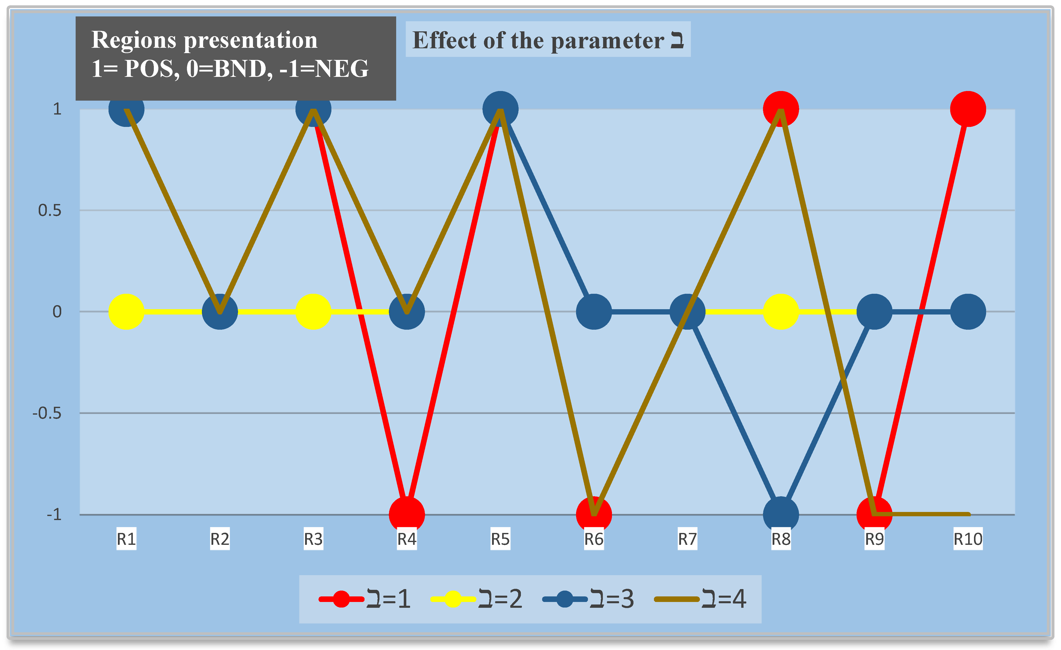
The parameter ℶ holds significant importance in Aczel–Alsina aggregation operators as it influences the outcomes. By manipulating the value of ℶ, which is greater than 0, different results can be achieved. Specifically, ℶ is set to 1, 2, 3, and 4 to explore the impact on decision regions, causing certain objects to shift positions. Notably, throughout this variation, 1 and 5 consistently remain in the positive region, demonstrating their reliability and suitability for investment. However, the positions of other objects exhibit variability. The implications of these alterations in the decision regions, along with their graphical representation, can be found in Table 6 and Figure 3, respectively.

7.4. Benefits of the Approach

The proposed approach offers several benefits, which are elaborated upon below.
1. 
Generalization: One of the key advantages of this approach is its greater level of generalization. It extends the theory of IFSs and provides a more inclusive framework. By reducing membership values and non-membership values to singletons, intuitionistic hesitant fuzzy sets can be converted into intuitionistic fuzzy sets.
6. 
Aczel–Alsina aggregation operators: The use of Aczel–Alsina aggregation operators is particularly advantageous for decision-making in fuzzy environments. These operators are simple yet effective, and they also consider the element of time. They have been designed specifically for novel data and are employed to aggregate information in a meaningful way.
7. 
Improved three-way decision (3WD) approach: Existing approaches in the literature, such as those proposed by Yao [28], are often considered traditional. In contrast, this model introduces new stages for 3WD, containing the plan of Aczel–Alsina aggregation operators and the utilization of interval-valued equivalence classes for approximation spaces. These enhancements make the approach more efficient thanexisting methods.
8. 
Business investment decision-making: Making optimal investment decisions is a critical and challenging task for investors, especially in a business context. In this study, we address this problem by establishing an approach that incorporates multiple companies. The effect of the parameter ℶ is demonstrated, showcasing the variation in the positive, negative, and boundary regions. This information aids in making well-informed investment decisions.
Overall, the proposed approach offers a more generalized framework, leverages suitable aggregation operators, introduces novel steps for 3WD, and provides valuable insights for investment decision-making.

8. Comparative Analysis

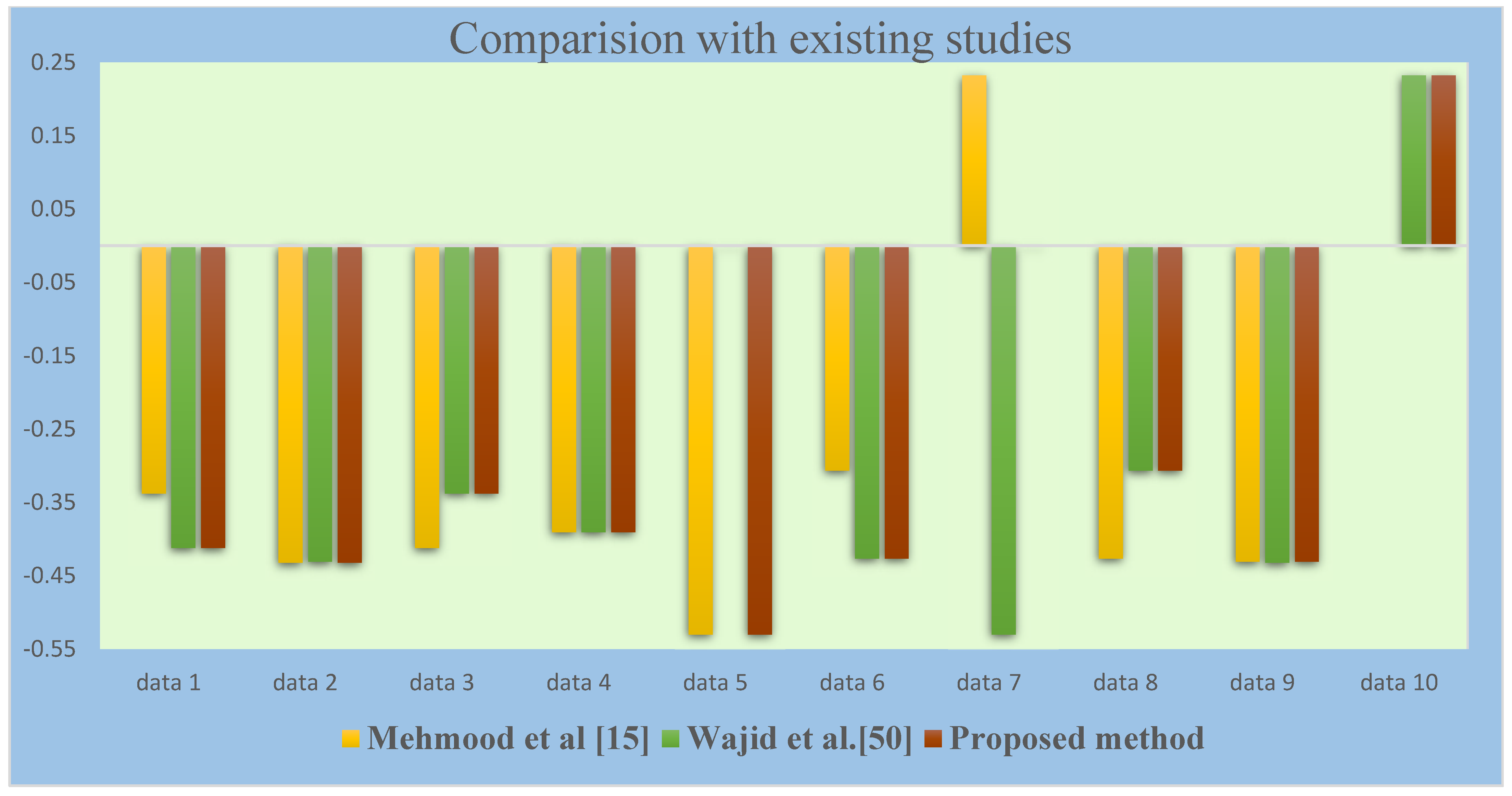
In this section, we will provide a concise synopsis of the comparison analysis conducted using Table 1 and Table 7. We aim to assess the preferences of our proposed approach in comparison to existing methods. The information system described in Table 1 serves as the basis for this comparative analysis, which includes the approaches referenced in [15,18,45,46,47,48,49,50].
  • Table 7 and Table 8 encompass the comparison analysis conducted between existing approaches and our proposed approaches.
  • In contrast to the works of Mahmood et al. [15] and Wajid et al. [50], our proposed model exhibits a higher level of flexibility in delivering acceptance outcomes for both multiple-attribute decision-making (MADM) and three-way decision (3WD).
  • Our observations further indicate that [18,45,46,47] demonstrate an effective ability to handling IF and HF information. However, it is important to note that there are specific scenarios where these models may not be suitable. This emphasizes the reliability and efficacy of our established idea for decision-makers.
  • The data presented in Table 7 shed light on the contributions of Senapati et al. [45,47], who devised interval-valued IFAAW, interval-valued IFAAWG, and HFAAWA operators specifically for interval-valued intuitionistic fuzzy information and hesitant fuzzy data. Nonetheless, comparative studies have revealed that these approaches lack effectiveness when dealing with intuitionistic hesitant fuzzy data. Hence, our proposed approach provides a solution that addresses more intricate and ambiguous scenarios.
Table 7. Comparison analysis of alternatives by ranking.
ApproachesInformationRanking
Xu, et al. [46]IFSsNo
Xu, et al. [18]IFSsNo
Senapati, et al. [45]Interval-IFSsNo
Senapati, et al. [47]HFSsNo
Seikh, et al. [48]IFSsNo
Ahmmad, et al. [49]IFRSsNo
Mahmood, et al. [15]IHFSs 7 > 10 > 6 > 1 > 4 > 3 > 8 > 9 > 2 > 5
Wajid, et al. [50]IHFSs 10 > 5 > 8 > 3 > 4 > 1 > 6 > 2 > 9 > 7
Proposed approachIHFSs 10 > 7 > 8 > 3 > 4 > 1 > 6 > 9 > 2 > 5
Table 8. Comparison analysis for 3WD-making.
ApproachesInformationRanking
Xu, et al. [46]IFSsNoNoNo
Xu, et al. [18]IFSsNoNoNo
Senapati, et al. [45]Interval-IFSsNoNoNo
Senapati, et al. [47]HFSsNoNoNo
Seikh, et al. [48]IFSsNoNoNo
Ahmmad, et al. [49]IFRSsNoNoNo
Mahmood, et al. [15]IHFSs { 1 , 3 , 5 } { 2 , 7 , 10 } { 4 , 6 , 8 , 9 }
Wajid, et al. [50]IHFSs { 1 , 3 , 5 } { 2 , 7 , 10 } { 4 , 6 , 8 , 9 }
Proposed approachIHFSs { 1 , 3 , 5 } { 2 , 7 , 10 } { 4 , 6 , 8 , 9 }
The Figure 4 Comparative analysis shows us a graphical representation of the results of given Table 7.

9. Conclusions

This paper primarily focuses on the three-way decision model and multiple-attribute decision-making, which are both highly influential frameworks employed for decision-making based on object attributes. These models have garnered considerable attention and adoption in various domains, such as business, medicine, and technology, due to their effectiveness in real-life situations. However, decision-makers often face challenges arising from limited data and time constraints. To tackle these difficulties, we leveraged the potential of IHFSs, which encompass both MG and NMG sets. Consequently, we proposed I H F A A H A ϣ operators specifically designed for multiple attribute decision making (MADM) and three-way decision (3WD) making, with the aim of providing a practical solution in such contexts.
In the article, we first reviewed the Aczel–Alsina T . N and T . C N in an IHF environment, explained some new operating rules for IHFNs, and examined at their characteristics. Then, with an understanding of these new functional laws, some exclusive AOs, for instance, the I H F A A W A ϣ operator, I H F A A O W A ϣ operator, and I H F A A H A ϣ operator were constructed to validate to the specifications where the assigned opinions are IHFNs. Moreover, the three-way decision made using the rough set approach was also generalized; for this purpose, we established the concept of interval-valued equivalence classes. The three-way decision concept is designed based on AOs and intuitionistic hesitant fuzzy sets. Additionally, we looked at the 3WD-making issue using the Aczel–Alsina aggregating operators and IHF information. We managed the operators to create various approaches to determine the IHF 3WD troubles. We also proposed a novel model for MADM using the series of aggregation operators for IHFNs. Last, a useful example was prestented to prove the determined method and to establish its feasibility and proficiency.
To validate and establish the authenticity, authenticity, and efficiency of our developed model, we conducted a thorough comparison with existing models. The models and techniques we devised have practical applications in diverse fields, such as networking analysis, risk assessment, and cognitive science, particularly in scenarios characterized by uncertainty. Moving forward, our future investigations will delve into the application of our novel techniques in the realm of multi-criteria development within the fuzzy environment. We will also explore the underlying concept of intuitionistic hesitant fuzzy connection information [51,52] in relation to our suggested methods. Additionally, our ongoing research involves the utilization of a temporal intuitionistic fuzzy system [53,54,55] as an avenue for further exploration.

Author Contributions

Conceptualization, W.A., T.S., H.G.T., F.A., M.Z.U. and M.M.H.; methodology, W.A. and T.S.; software, W.A.; validation, W.A., T.S., H.G.T., F.A., M.Z.U. and M.M.H.; formal analysis, W.A. and T.S.; investigation, W.A., T.S., H.G.T., F.A., M.Z.U. and M.M.H.; resources, M.Z.U. and M.M.H.; data curation, W.A., T.S. and H.G.T.; writing—original draft preparation, W.A., T.S., H.G.T., F.A., M.Z.U. and M.M.H.; writing—review and editing, M.Z.U. and M.M.H.; visualization, W.A.; funding acquisition, M.M.H. All authors have read and agreed to the published version of the manuscript.

Funding

The authors are grateful to King Saud University, Riyadh, Saudi Arabia for funding this work through Researchers Supporting Project Number (RSP2023R18).

Data Availability Statement

Not Applicable.

Conflicts of Interest

The authors declare no conflict of interest.

References

  1. Ardil, C. Vague Multiple Criteria Decision Making Analysis Method for Fighter Aircraft Selection. Int. J. Aerosp. Mech. Eng. 2022, 16, 133–142. [Google Scholar]
  2. Bourahla, M. Using Rough Set Theory for Reasoning on Vague Ontologies. Int. J. Intell. Syst. Appl. 2022, 14, 21–36. [Google Scholar] [CrossRef]
  3. Zadeh, L. Fuzzy sets. Inf. Control 1965, 8, 338–353. [Google Scholar] [CrossRef] [Green Version]
  4. Zhang, L.; Zhang, B. The Quotient Space Theory of Problem Solving. Fundam. Inform. 2004, 59, 287–298. [Google Scholar] [CrossRef]
  5. Pawlak, Z. Rough set theory and its applications to data analysis. Cybern. Syst. 1998, 29, 661–688. [Google Scholar] [CrossRef]
  6. Saraji, M.K.; Mardani, A.; Köppen, M.; Mishra, A.R.; Rani, P. An extended hesitant fuzzy set using SWARA-MULTIMOORA approach to adapt online education for the control of the pandemic spread of COVID-19 in higher education institutions. Artif. Intell. Rev. 2021, 55, 181–206. [Google Scholar] [CrossRef]
  7. Onbaşıoğlu, Ş.; Varol, B.P. Intuitionistic Fuzzy Metric-like Spaces and Fixed-Point Results. Mathematics 2023, 11, 1902. [Google Scholar] [CrossRef]
  8. Bera, J.; Das, K.C.; Samanta, S.; Lee, J.-G. Connectivity Status of Intuitionistic Fuzzy Graph and Its Application to Merging of Banks. Mathematics 2023, 11, 1949. [Google Scholar] [CrossRef]
  9. Atanassov, K.T. On Intuitionistic Fuzzy Sets Theory; Springer: Berlin/Heidelberg, Germany, 2012; Volume 283. [Google Scholar]
  10. Torra, V. Hesitant fuzzy sets. Int. J. Intell. Syst. 2010, 25, 529–539. [Google Scholar] [CrossRef]
  11. Garg, H.; Keikha, A. Various aggregation operators of the generalized hesitant fuzzy numbers based on Archimedean t-norm and t-conorm functions. Soft Comput. 2022, 26, 13263–13276. [Google Scholar] [CrossRef]
  12. Resti, Y.; Irsan, C.; Neardiaty, A.; Annabila, C.; Yani, I. Fuzzy Discretization on the Multinomial Naïve Bayes Method for Modeling Multiclass Classification of Corn Plant Diseases and Pests. Mathematics 2023, 11, 1761. [Google Scholar] [CrossRef]
  13. Guo, Z.; Liu, S. Study on the Selection of Pharmaceutical E-Commerce Platform Considering Bounded Rationality under Probabilistic Hesitant Fuzzy Environment. Mathematics 2023, 11, 1859. [Google Scholar] [CrossRef]
  14. Albaity, M.; Mahmood, T.; Ali, Z. Impact of Machine Learning and Artificial Intelligence in Business Based on Intuitionistic Fuzzy Soft WASPAS Method. Mathematics 2023, 11, 1453. [Google Scholar] [CrossRef]
  15. Mahmood, T.; Ali, W.; Ali, Z.; Chinram, R. Power Aggregation Operators and Similarity Measures Based on Improved Intuitionistic Hesitant Fuzzy Sets and their Applications to Multiple Attribute Decision Making. Comput. Model. Eng. Sci. 2021, 126, 1165–1187. [Google Scholar] [CrossRef]
  16. Yager, R.R. Generalized OWA aggregation operators. Fuzzy Optim. Decis. Mak. 2004, 3, 93–107. [Google Scholar] [CrossRef]
  17. Yager, R.R. Prioritized aggregation operators. Int. J. Approx. Reason. 2008, 48, 263–274. [Google Scholar] [CrossRef] [Green Version]
  18. Xu, Z.; Yager, R.R. Some geometric aggregation operators based on intuitionistic fuzzy sets. Int. J. Gen. Syst. 2006, 35, 417–433. [Google Scholar] [CrossRef]
  19. Zhang, H.; Wei, G.; Chen, X. Spherical fuzzy Dombi power Heronian mean aggregation operators for multiple attribute group decision-making. Comput. Appl. Math. 2022, 41, 1–54. [Google Scholar] [CrossRef]
  20. Senapati, T.; Chen, G.; Yager, R.R. Aczel–Alsina aggregation operators and their application to intuitionistic fuzzy multiple attribute decision making. Int. J. Intell. Syst. 2021, 37, 1529–1551. [Google Scholar] [CrossRef]
  21. Ayub, N.; Malik, A. Dual hesitant fuzzy Bonferroni means and its applications in decision-making. Ital. J. Pure Appl. Math. 2022, 48, 32–53. [Google Scholar]
  22. Hadi, A.; Khan, W.; Khan, A. A novel approach to MADM problems using Fermatean fuzzy Hamacher aggregation operators. Int. J. Intell. Syst. 2021, 36, 3464–3499. [Google Scholar] [CrossRef]
  23. Yao, Y. Three-Way Decisions and Cognitive Computing. Cogn. Comput. 2016, 8, 543–554. [Google Scholar] [CrossRef]
  24. Yao, Y. An outline of a theory of three-way decisions. In Proceedings of the International Conference on Rough Sets and Current Trends in Computing, Chengdu, China, 17–20 August 2012; Springer: Berlin/Heidelberg, Germany, 2012. [Google Scholar]
  25. Yao, Y. The geometry of three-way decision. Appl. Intell. 2021, 51, 6298–6325. [Google Scholar] [CrossRef]
  26. Mehmood, A.; Shaikh, I.U.H.; Ali, A. Application of Deep Reinforcement Learning for Tracking Control of 3WD Omnidirectional Mobile Robot. Inf. Technol. Control. 2021, 50, 507–521. [Google Scholar] [CrossRef]
  27. Zhang, C.; Ding, J.; Li, D.; Zhan, J. A novel multi-granularity three-way decision making approach in q-rung orthopair fuzzy information systems. Int. J. Approx. Reason. 2021, 138, 161–187. [Google Scholar] [CrossRef]
  28. Yao, Y.; Deng, X. Sequential three-way decisions with probabilistic rough sets. In Proceedings of the IEEE 10th International Conference on Cognitive Informatics and Cognitive Computing (ICCI-CC’11), Banff, AB, Canada, 18–20 August 2011. [Google Scholar]
  29. Zhao, T.; Zhang, Y.; Miao, D. Intuitionistic Fuzzy-Based Three-Way Label Enhancement for Multi-Label Classification. Mathematics 2022, 10, 1847. [Google Scholar] [CrossRef]
  30. Liu, D.; Yao, Y.; Li, T. Three-way investment decisions with decision-theoretic rough sets. Int. J. Comput. Intell. Syst. 2011, 4, 66–74. [Google Scholar]
  31. Zhang, K.; Dai, J. A novel TOPSIS method with decision-theoretic rough fuzzy sets. Inf. Sci. 2022, 608, 1221–1244. [Google Scholar] [CrossRef]
  32. Qian, Y.; Zhang, H.; Sang, Y.; Liang, J. Multigranulation decision-theoretic rough sets. Int. J. Approx. Reason. 2014, 55, 225–237. [Google Scholar] [CrossRef]
  33. Ali, Z.; Mahmood, T.; Smarandache, F. Three-Way Decisions with Single-Valued Neutrosophic Uncertain Linguistic Decision-Theoretic Rough Sets Based on Generalized Maclaurin Symmetric Mean Operators. Neutrosophic Oper. Res. 2021, 71–101. [Google Scholar] [CrossRef]
  34. Abdullah, S.; Almagrabi, A.O.; Ullah, I. A New Approach to Artificial Intelligent Based Three-Way Decision Making and Analyzing S-Box Image Encryption Using TOPSIS Method. Mathematics 2023, 11, 1559. [Google Scholar] [CrossRef]
  35. Menger, K. Statistical metrics. Proc. Natl. Acad. Sci. USA 1942, 28, 535. [Google Scholar] [CrossRef] [Green Version]
  36. Deschrijver, G.; Cornelis, C.; Kerre, E.E. On the representation of intuitionistic fuzzy t-norms and t-conorms. IEEE Trans. Fuzzy Syst. 2004, 12, 45–61. [Google Scholar] [CrossRef]
  37. Drossos, C. Generalized t-norm structures. Fuzzy Sets Syst. 1999, 104, 53–59. [Google Scholar] [CrossRef]
  38. Boixader, D.; Recasens, J. Vague and fuzzy t-norms and t-conorms. Fuzzy Sets Syst. 2022, 433, 156–175. [Google Scholar] [CrossRef]
  39. Ashraf, S.; Abdullah, S.; Aslam, M.; Qiyas, M.; Kutbi, M.A. Spherical fuzzy sets and its representation of spherical fuzzy t-norms and t-conorms. J. Intell. Fuzzy Syst. 2019, 36, 6089–6102. [Google Scholar] [CrossRef]
  40. Pap, E.; Bošnjak, Z.; Bošnjak, S. Application of fuzzy sets with different t-norms in the interpretation of portfolio matrices in strategic management. Fuzzy Sets Syst. 2000, 114, 123–131. [Google Scholar] [CrossRef]
  41. Rasuli, R. Fuzzy Equivalence Relation, Fuzzy Congrunce Relation and Fuzzy Normal Subgroups on Group G over T-Norms. Asian J. Fuzzy Appl. Math. 2019, 7. [Google Scholar] [CrossRef] [Green Version]
  42. Klement, E.P.; Mesiar, R.; Pap, E. Generated triangular norms. Kybernetika 2000, 36, 363–377. [Google Scholar]
  43. Aczél, J.; Alsina, C. Characterizations of some classes of quasilinear functions with applications to triangular norms and to synthesizing judgements. Aequ. Math. 1982, 25, 313–315. [Google Scholar] [CrossRef]
  44. Hussain, A.; Ullah, K.; Yang, M.-S.; Pamucar, D. Aczel-Alsina Aggregation Operators on T-Spherical Fuzzy (TSF) Information With Application to TSF Multi-Attribute Decision Making. IEEE Access 2022, 10, 26011–26023. [Google Scholar] [CrossRef]
  45. Senapati, T.; Chen, G.; Mesiar, R.; Yager, R.R. Novel Aczel–Alsina operations-based interval-valued intuitionistic fuzzy aggregation operators and their applications in multiple attribute decision-making process. Int. J. Intell. Syst. 2021, 37, 5059–5081. [Google Scholar] [CrossRef]
  46. Xu, Z. Intuitionistic Fuzzy Aggregation Operators. IEEE Trans. Fuzzy Syst. 2007, 15, 1179–1187. [Google Scholar] [CrossRef]
  47. Senapati, T.; Chen, G.; Mesiar, R.; Yager, R.R.; Saha, A. Novel Aczel–Alsina operations-based hesitant fuzzy aggregation operators and their applications in cyclone disaster assessment. Int. J. Gen. Syst. 2022, 51, 511–546. [Google Scholar] [CrossRef]
  48. Seikh, M.R.; Mandal, U. Intuitionistic fuzzy Dombi aggregation operators and their application to multiple attribute decision-making. Granul. Comput. 2019, 6, 473–488. [Google Scholar] [CrossRef]
  49. Ahmmad, J.; Mahmood, T.; Mehmood, N.; Urawong, K.; Chinram, R. Intuitionistic Fuzzy Rough Aczel-Alsina Average Aggregation Operators and Their Applications in Medical Diagnoses. Symmetry 2022, 14, 2537. [Google Scholar] [CrossRef]
  50. Ali, W.; Shaheen, T.; Toor, H.G.; Akram, F.; Uddin, Z.; Hassan, M.M. Selection of Investment Policy Using a Novel Three-Way Group Decision Model under Intuitionistic Hesitant Fuzzy Sets. Appl. Sci. 2023, 13, 4416. [Google Scholar] [CrossRef]
  51. Ali, W.; Shaheen, T.; Haq, I.U.; Toor, H.G.; Akram, F.; Jafari, S.; Uddin, Z.; Hassan, M.M. Multiple-Attribute Decision Making Based on Intuitionistic Hesitant Fuzzy Connection Set Environment. Symmetry 2023, 15, 778. [Google Scholar] [CrossRef]
  52. Radenovic, S.; Ali, W.; Shaheen, T.; Haq, I.U.; Akram, F.; Toor, H. Multiple Attribute Decision-Making Based on Bonferroni MeanOperatorsunderSquare Root Fuzzy Set Environment. J. Comput. Cogn. Eng. 2022. [Google Scholar] [CrossRef]
  53. Atanassov, K. On Intuitionistic Fuzzy Temporal Topological Structures. Axioms 2023, 12, 182. [Google Scholar] [CrossRef]
  54. Wang, Z.; Miao, D. Spatial-temporal single object tracking with three-way decision theory. Int. J. Approx. Reason. 2023, 154, 38–47. [Google Scholar] [CrossRef]
  55. Ul Haq, I.; Shaheen, T.; Ali, W.; Senapati, T. A Novel SIR Approach to Closeness Coefficient-Based MAGDM Problems Using Pythagorean Fuzzy Aczel–Alsina Aggregation Operators for Investment Policy. Discret. Dyn. Nat. Soc. 2022, 2022, 5172679. [Google Scholar] [CrossRef]
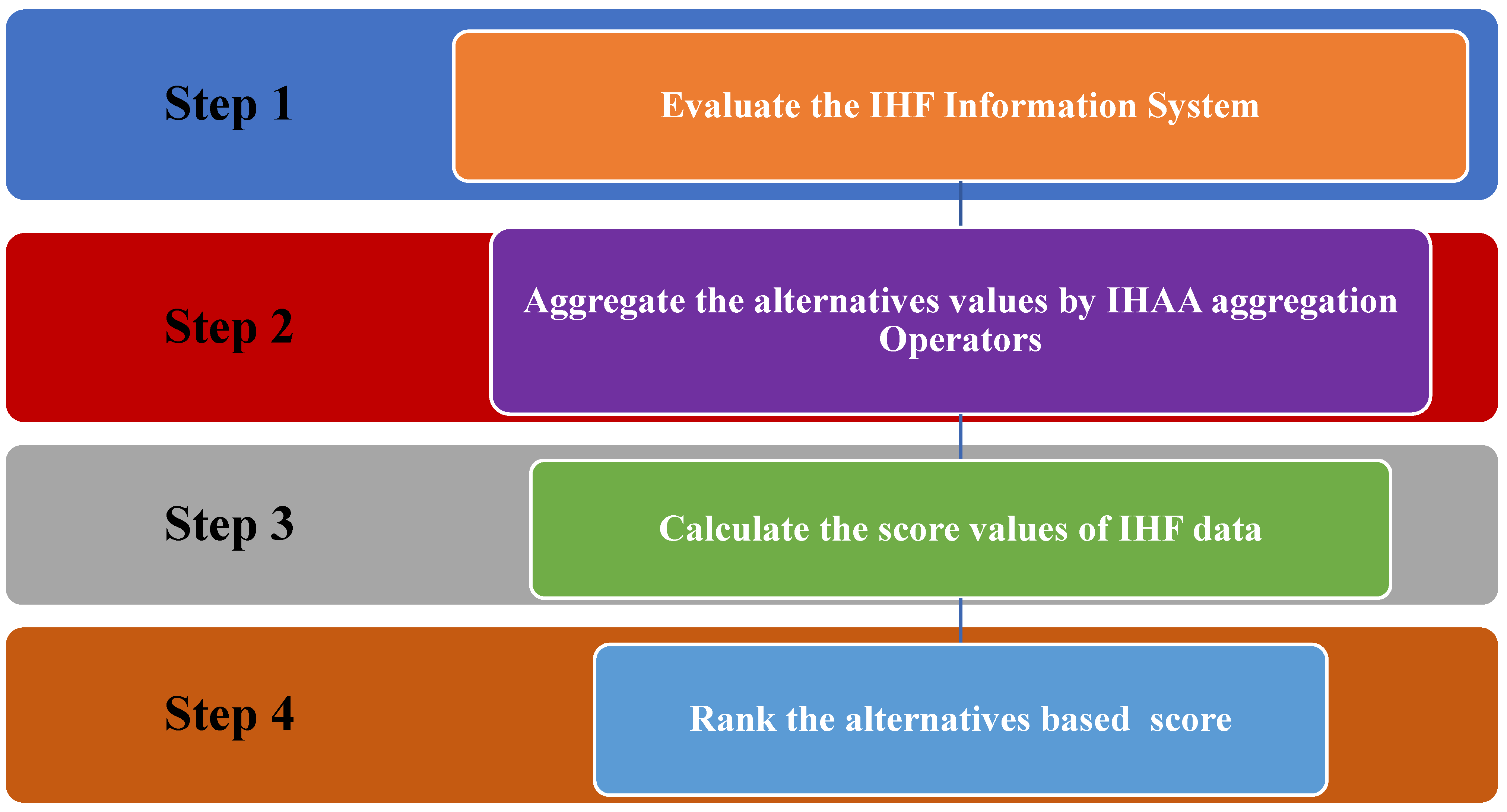
Figure 1. Flow chart of MADM.
Mathematics 11 02768 g001
Figure 2. Flow chart of three-way decision process.
Mathematics 11 02768 g002
Figure 3. Geometric representation of variations in regions.
Mathematics 11 02768 g003
Figure 4. Comparative analysis.
Mathematics 11 02768 g004
Table 1. Intuitionistic hesitant information system.
G 1 G 2 G 3 G 4
1 { { 0.13 , 0.31 } , { 0.12 , 0.43 } } { { 0.32 , 0.13 } , { 0.22 , 0.14 } } { { 0.0 , 0.13 } , { 0.19 , 0.17 } } { { 0.23 , 0.14 } , { 0.13 , 0.12 } }
2 { { 0.03 , 0.12 } , { 0.09 , 0.19 } } { { 0.0 , 0.14 } , { 0.12 , 0.23 } } { { 0.1 , 0.14 } , { 0.23 , 0.32 } } { { 0.11 , 0.21 } , { 0.01 , 0.34 } }
3 { { 0.02 , 0.32 } , { 0.1 , 0.12 } } { { 0.12 , 0.29 } , { 0.22 , 0.19 } } { { 0.21 , 0.52 } , { 0.18 , 0.23 } } { { 0.23 , 0.16 } , { 0.07 , 0.23 } }
4 { { 0.21 , 0.13 } , { 0.12 , 0.12 } } { { 0.13 , 0.14 } , { 0.15 , 0.13 } } { { 0.0 , 0.12 } , { 0.15 , 0.34 } } { { 0.31 , 0.23 } , { 0.29 , 0.22 } }
5 { { 0.21 , 0.22 } , { 0.19 , 0.9 } } { { 0.1 , 0.14 } , { 0.19 , 0.2 } } { { 0.24 , 0.21 } , { 0.23 , 0.56 } } { { 0.32 , 0.15 } { 0.12 , 0.28 } }
6 { { 0.14 , 0.03 } , { 0.17 , 0.11 } } { { 0.21 , 0.03 } , { 0.11 , 0.12 } } { { 0.32 , 0.07 } , { 0.72 , 0.2 } } { { 0.27 , 0.12 } { 0.12 , 0.34 } }
7 { { 0.12 , 0.05 } , { 0.09 , 0.15 } } { { 0.05 , 0.13 } , { 0.13 , 0.13 } } { { 0.11 , 0.14 } , { 0.65 , 0.01 } } { { 0.22 , 0.06 } , { 0.22 , 0.26 } }
8 { { 0.13 , 0.21 } , { 0.13 , 0.36 } } { { 0.17 , 0.46 } , { 0.0 , 0.12 } } { { 0.18 , 0.19 } , { 0.08 , 0.14 } } { { 0.43 , 0.12 } , { 0.12 , 0.17 } }
9 { { 0.11 , 0.22 } , { 0.04 , 0.32 } } { { 0.07 , 0.09 } , { 0.17 , 0.23 } } { { 0.07 , 0.14 } , { 0.36 , 0.32 } } { { 0.22 , 0.27 } , { 0.11 , 0.09 } }
10 { { 0.09 , 0.24 } , { 0.09 , 0.11 } } { { 0.11 , 0.05 } , { 0.22 , 0.24 } } { { 0.12 , 0.29 } , { 0.19 , 0.22 } } { { 0.13 , 0.08 } , { 0.12 , 0.05 } }
Table 2. Aggregation of the information of alternatives using I H F A A W A .
Objects\Operators I H F A A W A ϣ
1 ( 0.082465 ,   0.494573 )
2 ( 0.043971 ,   0.476253 )
3 ( 0.110119 ,   0.447884 )
4 ( 0.068807 ,   0.459562 )
5 ( 0.091355 ,   0.621606 )
6 ( 0.062992 ,   0.489813 )
7 ( 0.046929 ,   0.469006 )
8 ( 0.106456 ,   0.412838 )
9 ( 0.064632 ,   0.495332 )
10 ( 0.066298 ,   0.430755 )
Table 3. Score values of the objects.
Objects Score   Values
1 0.412108
2 0.432282
3 0.337765
4 0.390755
5 0.530251
6 0.426821
7 0.0000284
8 0.306382
9 0.4307
10 0.232225
Table 4. Ranking of alternatives.
OperatorRanking
I H F A A W A ϣ 10 > 7 > 8 > 3 > 4 > 1 > 6 > 9 > 2 > 5
Table 5. Intuitionistic hesitant conditional and decision attribute information.
G 1 G 2 G 3 G 4 D
1 { { 0.13 , 0.31 } , { 0.12 , 0.43 } } { { 0.32 , 0.13 } , { 0.22 , 0.14 } } { { 0.0 , 0.13 } , { 0.19 , 0.17 } } { { 0.23 , 0.14 } , { 0.13 , 0.12 } } Yes
2 { { 0.03 , 0.12 } , { 0.09 , 0.19 } } { { 0.0 , 0.14 } , { 0.12 , 0.23 } } { { 0.1 , 0.14 } , { 0.23 , 0.32 } } { { 0.11 , 0.21 } , { 0.01 , 0.34 } } Yes
3 { { 0.02 , 0.32 } , { 0.1 , 0.12 } } { { 0.12 , 0.29 } , { 0.22 , 0.19 } } { { 0.21 , 0.52 } , { 0.18 , 0.23 } } { { 0.23 , 0.16 } , { 0.07 , 0.23 } } Yes
4 { { 0.21 , 0.13 } , { 0.12 , 0.12 } } { { 0.13 , 0.14 } , { 0.15 , 0.13 } } { { 0.0 , 0.12 } , { 0.15 , 0.34 } } { { 0.31 , 0.23 } , { 0.29 , 0.22 } } No
5 { { 0.21 , 0.22 } , { 0.19 , 0.9 } } { { 0.1 , 0.14 } , { 0.19 , 0.2 } } { { 0.24 , 0.21 } , { 0.23 , 0.56 } } { { 0.32 , 0.15 } { 0.12 , 0.28 } } Yes
6 { { 0.14 , 0.03 } , { 0.17 , 0.11 } } { { 0.21 , 0.03 } , { 0.11 , 0.12 } } { { 0.32 , 0.07 } , { 0.72 , 0.2 } } { { 0.27 , 0.12 } { 0.12 , 0.34 } } No
7 { { 0.12 , 0.05 } , { 0.09 , 0.15 } } { { 0.05 , 0.13 } , { 0.13 , 0.13 } } { { 0.11 , 0.14 } , { 0.65 , 0.01 } } { { 0.22 , 0.06 } , { 0.22 , 0.26 } } No
8 { { 0.13 , 0.21 } , { 0.13 , 0.36 } } { { 0.17 , 0.46 } , { 0.0 , 0.12 } } { { 0.18 , 0.19 } , { 0.08 , 0.14 } } { { 0.43 , 0.12 } , { 0.12 , 0.17 } } Yes
9 { { 0.11 , 0.22 } , { 0.04 , 0.32 } } { { 0.07 , 0.09 } , { 0.17 , 0.23 } } { { 0.07 , 0.14 } , { 0.36 , 0.32 } } { { 0.22 , 0.27 } , { 0.11 , 0.09 } } No
10 { { 0.09 , 0.24 } , { 0.09 , 0.11 } } { { 0.11 , 0.05 } , { 0.22 , 0.24 } } { { 0.12 , 0.29 } , { 0.19 , 0.22 } } { { 0.13 , 0.08 } , { 0.12 , 0.05 } } No
Table 6. Effect of parameter .
Positive RegionsNegative RegionsBoundary Regions
= 1 { 1 , 3 , 5 , 8 } { 4 , 6 , 9 , 10 } { 2 , 7 }
= 2 { 1 , 5 } { } { 2 , 3 , 4 , 6 , 7 , 8 , 9 , 10 }
= 3 { 1 , 3 , 5 } { 8 } { 2 , 4 , 6 , 7 , 9 , 10 }
= 4 { 1 , 3 , 5 , 8 } { 6 , 9 , 10 } { 2 , 4 , 7 }
Disclaimer/Publisher’s Note: The statements, opinions and data contained in all publications are solely those of the individual author(s) and contributor(s) and not of MDPI and/or the editor(s). MDPI and/or the editor(s) disclaim responsibility for any injury to people or property resulting from any ideas, methods, instructions or products referred to in the content.