1. Introduction
Queueing theory is a rapidly developing branch of applied probability that helps solve problems related to the sharing and scheduling of finite resources that have to be used by competing users. Systems with heterogeneous customers have been investigated less in the existing queueing literature. The varying requirements of several types of customers for the required system resource, indicators of the quality of service, and their different importance and value all lead to their needing different treatments. In particular, a powerful tool for the enhancement of the operation of such systems is the assignment of different priorities in accessing the system resources for different types of customers. The theory of priority queues is pretty well developed in the case of single-server queues (see, e.g., [
1,
2,
3,
4,
5]). However, the operation of many real-world systems can be adequately described only by multi-server priority queueing systems. The problem of optimal management in such systems is much more complicated than in single-server systems due to the larger dimensionality of the stochastic process that describes the dynamics of the system. However, the importance of consideration of such priority queueing systems made them a popular subject of research; see, e.g., the papers [
6,
7,
8,
9,
10,
11,
12,
13,
14,
15,
16] published within the last two years.
There are a lot of various priority schemes (preemptive and non-preemptive, alternating, static and dynamic, changing and accumulating, etc.) known in the literature; some references can be found, e.g., in [
17]. All these schemes have their own advantages and disadvantages. For example, the static priorities assuming strict adherence to the established rules of picking up from the queue are more easily realized in real systems. The preemptive priorities suggesting service interruption in the case of the arrival of a customer who has a higher priority than the one receiving service are fine for high-priority customers but are discriminatory with respect to low-priority customers. The dynamic priorities (see, e.g., [
18,
19],) give more flexibility but require efforts to monitor the system states. Therefore, to better manage the operation of different real-world systems, different new priority schemes are generated in the literature. For example, the scheme proposed in [
17] suggests the maintenance of auxiliary finite input buffers with different rates of customer transfer to the main buffer. A proper choice of the capacity of the buffers and the corresponding rates allows one to reach any desired degree of non-preemptive priority for one class of customers over another. Another flexible scheme for providing non-preemptive priority was offered in [
20]. That scheme assumes the randomized choice of the next customer for service, with probabilities of choice depending on the length of the queue of the priority customers. The scheme was applied and analyzed for the single-server queue. In this paper, we extend the analysis to the case of a multi-server queue. It is worth noting that there exist works (see, e.g., [
21]) where a priority to certain flows, e.g., flows of handover users in cellular mobile networks or primary users in cognitive radio systems, is provided via different kinds of schemes of reservation of some servers of the multi-server queueing system for service of priority users. Here, we do not touch on such a possibility. Priority is provided via the proper strategy of customers picking up from the queues.
It is already well known that flows of customers receiving service in many telecommunication systems, contact centers, hospitals, etc., exhibit a so-called bursty nature. The instantaneous arrival rate may significantly fluctuate during system operation. This makes the very popular-in-the-literature, stationary Poisson model of the arrival process a poor descriptor of real flows. The use of this model is not suitable for reliable prediction of the main performance measures of the systems. It may lead to huge errors in the estimation of the required system resources sufficient for providing the desired quality of service. Therefore, in this paper, we assume that the arrival flows of two types of customers receiving service in the system are defined by the much more general Marked Markov Arrival Process (
), see, e.g., [
22,
23,
24]. The
is an extension of the Markov Arrival Process (
) for accounting for the possibility of heterogeneous customer arrivals. In contrast to the stationary Poisson arrival process, the
is suitable for modeling flows with a non-zero coefficient of correlation and high variation in inter-arrival times. For more information about the basic properties, particular cases, and possible applications, as well as about the analysis of the systems with the
, see, e.g., [
24,
25,
26,
27,
28,
29,
30,
31,
32,
33,
34,
35,
36,
37,
38,
39,
40,
41,
42,
43,
44]. The multi-server priority queues with
arrival process have been analyzed, e.g., in [
9,
13,
16,
17,
20,
45,
46,
47].
The model considered in this paper assumes a so-called phase-type (
) distribution of service times of both types (see, e.g., [
24,
48,
49,
50,
51,
52]). This distribution essentially generalizes the well-known exponential distribution but still allows us to obtain nice analytical results. It can be applied to approximate any non-negative random variable distribution. In particular, it allows taking into account the variance of a random variable while the exponential distribution has a coefficient of variation equal to 1. However, the use of this distribution instead of the exponential distribution for the description of, e.g., service time, leads to the necessity of extending the dimension of the state space of the Markovian process describing the dynamics of a queueing system. It is necessary to keep track of the state of the underlying process (phase) of the
distribution in each busy server. If the considered queueing system has many servers, it essentially complicates the analysis of the system. If the number of identical servers is equal to
N while the number of phases is equal to
then the direct way of accounting for the phase of the underlying processes of service on all servers leads to the necessity of operating with matrices of size
describing the dynamics of the service process. When at least one of the numbers
N and
M is relatively large (while the number
N of servers in real systems can be pretty large), operating with matrices of such a size can be difficult. This is why in this paper, we use another way to monitor the service process. This way assumes an account of the number of servers providing service at each of
M possible phases. In the case when
M is relatively small, the state space of the service processes becomes much smaller, namely,
For example, in many cases, the value of
M equal to 2 allows us to have a good catch on the variance of service time. For
the size of the matrices that have to be treated is equal to
, which may be much less than
This way of describing the service process in multi-server queues was offered in [
53,
54].
In those papers, the recursive formulas for the computation of the matrices defining transition rates of the multi-dimensional Markov process, which describes the service process in many servers without a service completion and at the moments of new service beginning or ending, are presented. Formulas for computation of these matrices for the value
n of the number of currently busy servers (among
N available servers),
depend on both
n and
This is not convenient, especially when it is required to make computations for several values of
N, e.g., in the process of computing the minimum required number
N of servers to guarantee the fixed values of the service quality indicators. In [
55], the formulas derived in [
53,
54] are modified to eliminate the use of the value of
N in recursive computations.
In the considered model, it is assumed that the parameters of
distribution of the service time of customers of different types may be different. To avoid the necessity of separately monitoring the number of each type of customer in service and make the analysis easier, we use the notation of the generalized phase-type distribution introduced in [
56,
57].
We take into consideration the possibility of customers departing from the buffers due to impatience. Many real-world systems are inherently characterized by the impatience of their customers. For example, customers (information units) in telecommunication networks can depart from the waiting area due to information obsolescence, users’ departure from the service zone, etc. In contact centers, impatience is explained by the psychology of users. In retail networks and health systems (such as blood banks or organ transplantation hospitals), impatience is explained by the restricted term of the suitability of the items required for service. Recent lists of related research on queues with impatient customers can be found, e.g., in [
58,
59,
60,
61].
Account of customers’ impatience makes the considered model potentially useful; beyond the evident applications in telecommunications, it is also useful in the following systems. When two competing flows of passengers or vehicles, which arrive from different directions, merge into one flow, a popular mechanism of merging implementation consists of admitting a certain percentage of users from one direction and another. The considered model can help answer the question of how to optimally redistribute the percentage when one of the queues becomes large. In call centers, agents simultaneously handle the voice requests, which are admitted via the buffer of a finite capacity, as well as the requests arriving via the Internet that are placed in the buffer of a potentially infinite capacity. Over time, agents select for service waiting voice requests and Internet requests in some proportion. However, when the buffer for voice requests becomes close to its capacity (exceeds some threshold) and there is a high risk of their loss, the agents can decrease the percentage of Internet users admitted for service and, correspondingly, increase the percentage of voice users.
The structure of this paper is as follows. In
Section 2, the model of the considered queueing system is completely defined. In
Section 3, a multi-dimensional Markov chain describes how the system operates. The generator of this chain is derived there, and the problems of the existence of the stationary distribution of this Markov chain and the computation of this distribution are briefly discussed. In
Section 4, formulas for the computation of some performance measures of the system are presented. Some numerical illustrations are presented in
Section 5. The paper is concluded in
Section 6.
2. Mathematical Model
We consider an
N-server queuing system with two buffers, the structure of which is displayed in
Figure 1.
The system processes customers of two types. The customer’s arrival in the system is described by the
which is defined by the underlying continuous-time Markov chain (
)
with the state space
, and the square matrices
and
of size
The negative diagonal entries of the matrix
define, up to the sign, the transition rates of the
from the corresponding states. The non-diagonal entries of the matrix
define the transition rates that do not lead to the arrival of any customer. The entries of the matrices
are the transition rates of the
that cause the arrival of a type-
l customer. More information about the
and its characteristics can be found, e.g., in [
24].
Let us denote the total customers’ arrival rate as
and type-
l customers’ arrival rate as
These intensities are determined by the formulas:
where the stationary probability vector
of process
is determined to be the one solution to the system
where the row vector
consists of 0 s and the column vector
consists of 1 s.
The service time of a type-
customer has the phase-type distribution
that is defined by the underlying continuous-time
with the state space
, the vector
and the matrix
. The stochastic row vector
determines the initial state of the process
at the service beginning epoch, and the subgenerator
defines rates of transition of the process
inside the state space
The service time finishes when the process
transits to the absorbing state. The mean service time of type-
l customers is calculated as
For further details on the
distribution, its moments, and specific cases, see, for example, [
24].
If a customer of any type arrives at the system when there is a free server, this customer immediately starts service. A type-2 customer joins the infinite buffer if there are no available servers during its arrival period. Let us call this buffer Buffer-2. If there are no free servers during the arrival epoch of a type-1 customer, this customer tries to join the finite buffer of capacity R (Buffer-1). This trial will be successful in the case of a not full buffer. The arriving customer is lost forever if Buffer-1 is full during the type-1 customer arrival moment.
If during the epoch when some server finishes the service only customers of one type are in the buffers, the customer of such a type is chosen for service. If there are customers of two types in the buffers at the service completion moment, the type of customer that will receive service next is defined according to the following rule. If the number of type-1 customers in the buffer is less than the parameter K, a type-1 customer is chosen for service with the probability , and with the complimentary probability , a type-2 customer starts service. If the number of type-1 customers in the buffer is greater or equal to K, a type-1 customer is chosen for service with the probability and with the complimentary probability a type-2 customer starts service. We assume that the parameters , and are control parameters, and the task of modeling is to develop a mathematical tool that allows us to find the optimal values of these parameters according to a fixed cost criterion.
Each type of customer is assumed to be impatient and depart from the system without service if the service does not start within an exponentially distributed time since the arrival moment. The total rate of customers’ reneging from the corresponding buffer depends on the number of customers staying in the buffer. We assume that if there are r customers in Buffer-1, the total rate of reneging by type-1 customers is equal to If there are i customers in the infinite Buffer-2, the total rate of type-2 customers reneging is equal to and if
Let us analyze the stationary behavior of the model under consideration.
3. The Process of the System States and Its Analysis
The operation of the system under study is described by the following regular irreducible
-dimensional continuous-time
where at time
- •
is the number of customers in the system,
- •
is the number of type-1 customers in Buffer-1, ;
- •
is the number of type-1 customers in service, ;
- •
is the state of the underlying process of the of customers,
- •
is the number of type-1 customers at the m-th phase of the service process,
- •
is the number of type-2 customers at the l-th phase of the service process,
One can see that the process
is complicated, and its analysis may be cumbersome. To make the investigation easier, we use the notion of the generalized phase-type distribution, see, [
56,
57]. Instead of the separate consideration of service processes of each type of customer, we suggest that the customer’s service time at a server has the generalized
(
) distribution having the parameters
where the vectors
and
and subgenerator
S are defined by the formulas:
The duration of service is governed by the underlying process
with the state space
where
The state of the process
during the service beginning epoch is defined according to the probabilistic vector
if a type-
l customer starts service. The transition rates into the absorbing state (which implies service completion on one of the busy servers) are given by the entries of the column vector
The use of allows us to significantly simplify the process of defining the dynamics of the system and, correspondingly, its analysis.
The following regular irreducible continuous-time
can be used to describe the behavior of the system under consideration:
The meaning of the first three components
is the same as for the
. The component
of the vector-valued process
denotes the number of customers at the
m-th phase of the
service process at the moment
t,
To describe the transition rates of the let us first introduce the following auxiliary matrices:
define the rates of transitions of the process which do not lead to the end of service provided that i servers are busy;
define the transition probabilities of the process when i servers are busy and a type-1 or type-2 customer is chosen for service, correspondingly;
define the transitions rates of the process which cause the finish of service if i servers are busy;
define the rates of exit of the process from its states when i customers are in service.
Note that the recursive algorithms for the computation of the matrices
and
are available in paper [
55] and represent the advanced modification of the algorithms earlier presented in [
53,
54] and used, e.g., in [
62,
63,
64].
We enumerate the components of the in the direct lexicographic order and the components in reverse lexicographic order. All states with the value i of the first component are called the level i of the
We refer to the chain’s infinitesimal generator as G. All possible transition rates of the chain under study during an infinitesimally short time interval are defined as the entries of the generator G.
The notation used up until this point, and the new notation are compiled in
Table 1 for clarity and to make the description of the shape of the blocks of the generator
G simpler.
Theorem 1. The generator G has the following block-three-diagonal form: The non-zero blocks determining the transition rates from level i to level j are defined as follows: Proof.
By analyzing every potential transition of the during an interval of infinitesimal length and reconstructing the rates of such transitions in block matrix form, the proof of the theorem is implemented.
Customers of both types arrive and are served one at a time. The possibility of more than one consumer entering the system or being served in a moment that lasts an infinite amount of time is negligibly small. Hence, the generator G has a block-tridiagonal structure, and all the matrices are zero ones for i and j, such as
The negative diagonal entries of the matrices define, up to the sign, the total rate of leaving the corresponding state. The can exit from its state in the following cases:
(1) The underlying arrival process changes its state. The rates of the arrival process transitions are defined by the modulus of the corresponding diagonal entries of the matrix if (the system is empty), for and for Note that if the underlying arrival process makes a transition from some state to the same state with a type-1 customer arrival when Buffer-1 is full, the customer is lost, and the exit from the corresponding state does not occur. The rates of these transitions are given by the corresponding diagonal elements of the matrix
(2) The transition in the service process on one of the servers if there are busy servers in the system. The rates of these transitions are defined by the modulus of the corresponding diagonal elements of the matrix (if i customers are served in the system and there is no customer in the buffers) and by the matrix (if there are customers in service and in the buffers).
(3) One of the customers leaves the system due to impatience. If a type-1 customer leaves Buffer-1, the rates of these transitions are defined by the diagonal elements of the matrices for and of the matrix for The diagonal elements of the matrices and of the matrix , are the transition rates in the case of a type-2 customer leaving Buffer-2 due to impatience.
The non-diagonal elements of the blocks determine the transition rates of the that do not lead to the change in the number of customers in the system These transitions are as follows:
(1) The transition in the underlying arrival process without the arrival of a new customer (the rates of these transitions are the non-diagonal elements of the matrix if , for and for ).
(2) The arrival of a type-1 customer when N customers are being served in the system and Buffer-1 is full. Note that in such a case, the arriving customer is not accepted into the system. The corresponding rates are given by the elements of the matrix
(3) The change of the state of the service underlying process without service completion. The rates of these transitions are defined by the non-diagonal elements of the matrices (if i servers are busy but the buffers are empty) and of the matrices (if all servers are busy and there are customers in the buffers).
Using all these reasonings, we prove the form of the blocks
The elements of the matrices define the transition rates of the components of the that lead to the increase in the number of customers i in the system by one. This can happen only if a new customer is admitted to the system. When there is an idle server at an arrival moment, the transition rates are given by the elements of the matrices if type- customer arrives. The Kronecker multiplier reflects the fact that the arriving customer immediately starts service and, therefore, installation of the initial state of its service underlying process is required. If all servers are busy and an arriving type-1 customer joins Buffer-1, the elements of the matrices define the corresponding rates. The Kronecker multiplier is replaced here by the Kronecker multiplier because the new service does not start, and no transition of the service underlying process occurs. If a type-2 customer arrives at the system and is appended to Buffer-2, the corresponding rates are defined by the matrices and The matrices and reflect the fact of increasing the number of customers of the corresponding type in the buffer.
Next, we explain the formation of the blocks Their elements specify the transition rates of the components of the that lead to the decrease in the number of customers i in the system by one. These transitions are the following:
(1) A customer leaves the system due to the successful completion of the service. In this case, the corresponding rates are given as the elements of the matrices: (i) if there are i customers in service and the buffers are empty; (ii) and if all servers are busy and there are customers in the buffers, and a type-1 customer from Buffer-1 is chosen for service. Arguing in a similar way, we obtain matrices and that are defined the corresponding rates if a type-2 customer from Buffer-2 goes to service.
(2) A customer leaves the buffer due to impatience. If a type-1 customer leaves the system, the corresponding rates are given by the matrices for and by the matrix for If a type-2 customer is lost due to impatience, the related rates are given by the matrices and □
Having obtained the generator G of the it is possible to analyze this
Theorem 2. The is ergodic for any choice of the system parameters.
Proof.
It is easy to prove that, due to the assumption that
when
the following limits exist:
where the matrix
Here, ⨀ is the symbol of the Hadamard product of matrices, see [
67]. Therefore, the
fits the category of asymptotically quasi-Toeplitz Markov chains (
), see the definition of
in [
68].
As follows from [
68], a sufficient ergodicity condition of the
can be presented in the form
where the row-vector
can be obtained as the only solution
Since
one can see that the ergodicity condition turns to
and is fulfilled for any system parameters. □
It follows from Theorem 2, that the following limits (stationary probabilities of the states of the
) exist:
Let us form the row vectors of these probabilities enumerated in the same order as the components of the .
To obtain the stationary probability vectors
we have to find the only solution to the following system:
called the equilibrium or Chapman–Kolmogorov equations.
This system has an infinite number of unknowns and equations, and the generator
G does not have a level-independent structure. Thus, the problem of solving it is not easy. To solve this system, we recommend using the numerically stable algorithm presented in [
69]. In contrast to the general algorithm for
proposed in [
68] and designed for the upper-Hessenberg structure of the generator, the algorithm presented in [
69] is oriented, namely, to solving Chapman–Kolmogorov equations with the block tridiagonal structure of the generator, which has the
under study.
5. Numerical Example
In the numerical examples, we investigate the influence of the control parameters , , and K on the system operation. Since we can only present three-dimensional graphs, first, we examine the impact of the probabilities and on the main performance characteristics of the system under the fixed value of K. Then, we examine the influence of the probability and threshold K under the fixed value of probability Finally, we illustrate the importance of considering the system with the Namely, we illustrate that the approximation of the by the superposition of two stationary Poisson arrival processes may lead to significant errors in the evaluation of the key performance measures of the system.
Experiment 1. Let us assume that the customers arrive at the system according to the
arrival process that is defined by the following matrices:
The total rate of type-1 and type-2 customers’ arrivals to the system is
The coefficient of correlation of successive inter-arrival times in this arrival process is
the squared coefficient of variation is
. The average rate of type-1 customers’ arrivals
the average rate of type-2 customers’ arrivals is
.
The service process for type-1 customers is defined by the vector and the matrix The mean service time of type-1 customers is , and the squared coefficient of variation of the service times is 1.24723.
The service process for type-2 customers is defined by the vector and the matrix The mean service time of type-2 customers is 1, and the squared coefficient of variation of the service times is 1.61091.
Let us fix the control parameter and suggest that the number of servers N is equal to 4 and the capacity R of Buffer-1 is 10. Let the rates of impatience of type-1 customers and type-2 customers be defined as and respectively.
Let us vary the probability over the interval [0, 1] with step 0.05 and the probability over the interval also with step 0.05.
Figure 2 presents the dependence of the probability
of an arbitrary type-1 customer loss upon arrival due to Buffer-1 overflow on the parameters
and
One can see from
Figure 2 that in the considered example, the loss probability
decreases with growth in the probabilities
and
It is evident that when the probabilities
and
grow, type-1 customers are chosen for service more often, and the probability of meeting Buffer-1 full upon type-1 customer arrival decreases. The minimal value of the loss probability
is achieved for
(what corresponds to the standard non-preemptive priority of type-1 customers) and is equal to 0.000018797.
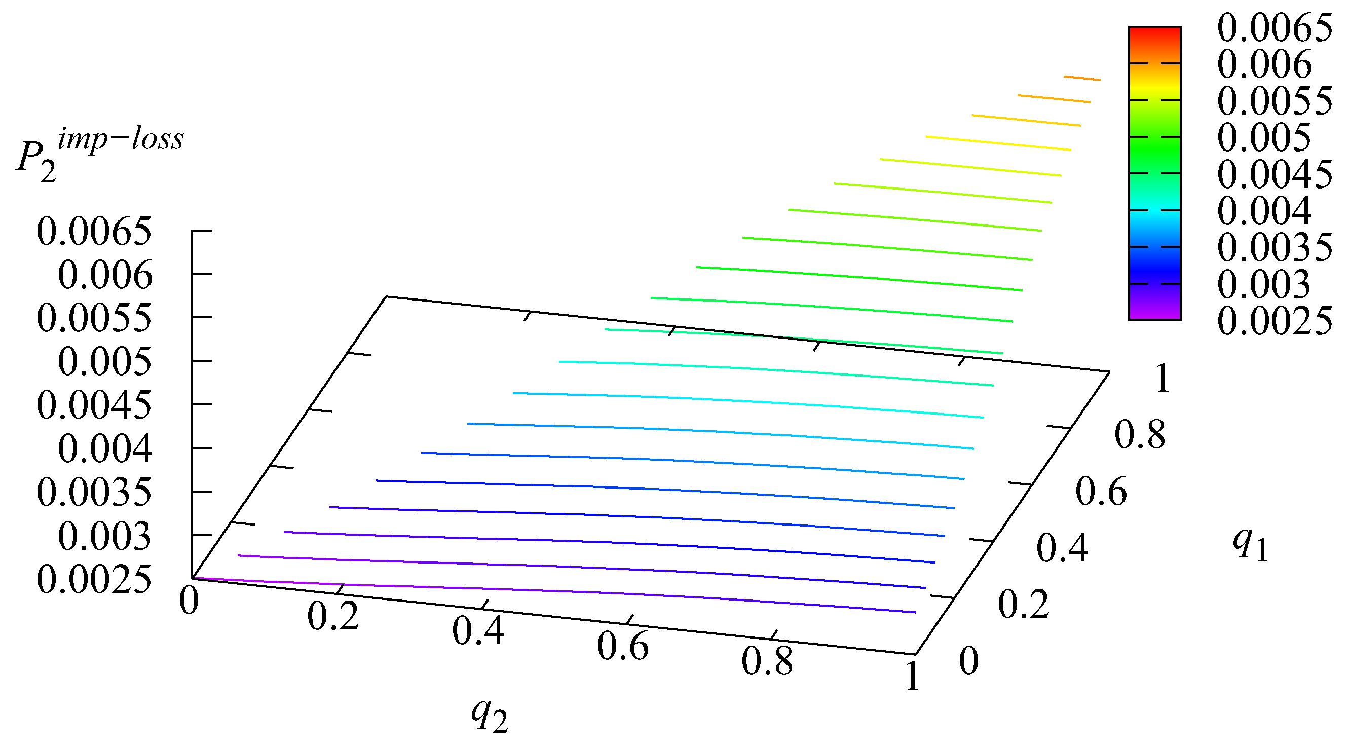
Figure 3 illustrates the dependence of the probability
of an arbitrary type-1 customer loss due to impatience on the parameters
and
One can see from
Figure 3 that in the considered example, the loss probability
sharply decreases with growth in the probability
and slightly decreases with growth in the probability
If the probability
is small and the number of customers in Buffer-1 is less than
, type-1 customers are rarely chosen for service. Thus, the number of type-1 customers staying in Buffer-1 is bigger for small values of
, and more customers leave the buffer due to impatience.
The dependence of the total probability
of an arbitrary type-1 customer loss on the parameters
and
is presented in
Figure 4.
The minimal value of the loss probability is also reached for and is equal to 0.0011.
Figure 5 illustrates the dependence of the probability
of an arbitrary type-2 customer loss due to impatience on the parameters
and
This probability evidently increases with growth in the probabilities and since the growth in these probabilities leads to worse conditions for type-2 customer service. More customers of this type stay in the infinite buffer, and consequently, more customers leave it due to impatience.
The dependence of the total probability
of an arbitrary customer loss on the parameters
and
is presented in
Figure 6.
In the considered case, the probability decreases with growth in the probability and increases with growth in the probability Note that for various input parameters, the dependence of the probability can be absolutely different. This is because the increase in probabilities implies lower probabilities of type-1 customers lost upon arrival and due to impatience but a higher probability of loss of type-2 customers. In the considered case, the minimal value of the loss probability is reached for and and is equal to 0.003326. So, to have minimal customer loss, we should always choose type-2 customers, if any, for service if the number of type-1 customers in the buffer is less than , and always choose type-1 customers otherwise. However, in real-world systems, the customers may have different importance to the system; that is, the charges for losing customers of different types may essentially differ.
Let us assume that the following economic criterion describes the system’s operating quality:
where
is a fee paid by the system in the case when a type-1 customer is lost, and
is a fee in the case when a type-2 customer from Buffer 2 is lost due to impatience.
The average losses of the system per unit of time are described by the economic criterion E. In order to optimize the system’s performance, we have to determine the probabilities and for which the economic criterion E assumes the lowest value.
Let us assume the following cost coefficients:
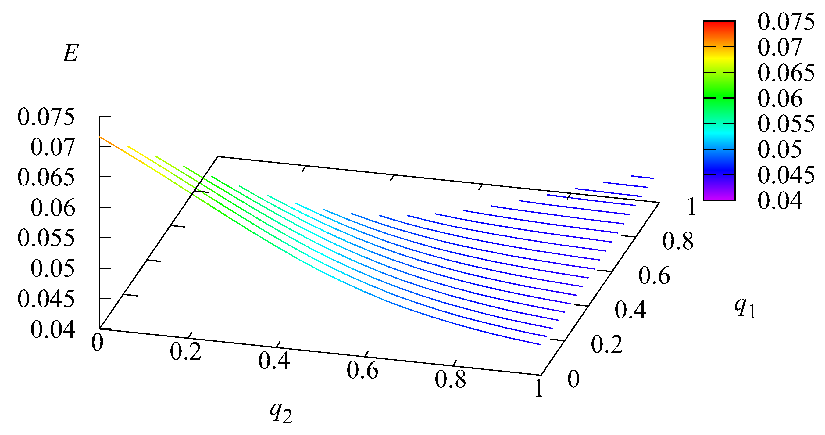
Figure 7 presents the dependence of the cost criterion
E on the parameters
and
.
The optimal value of the economic criterion is and is achieved when and Thus, if there are type-1 and type-2 customers in the buffers, it is reasonable to choose the type-1 customer for the next service with a probability of 0.35 if the number of type-1 customers in Buffer-1 is less than , and always choose the type-1 customer otherwise.
Experiment 2. In the second experiment, we analyze the dependence of the system performance measures on the control parameters and To this end, let us fix the probability , i.e., when the number of customers in the Buffer-1 exceeds the threshold then type-1 customers are always picked up for service. Additionally, let us increase the system load: we decrease the number of servers N to 3 and increase the capacity of Buffer-1 R from 10 to 20. The rest of the parameters are assumed to be the same as in the first experiment, including the arrival and service processes. We vary the control parameter K over the interval [2, 20] with step 1 and the probability over the interval [0, 1] with step 0.1.
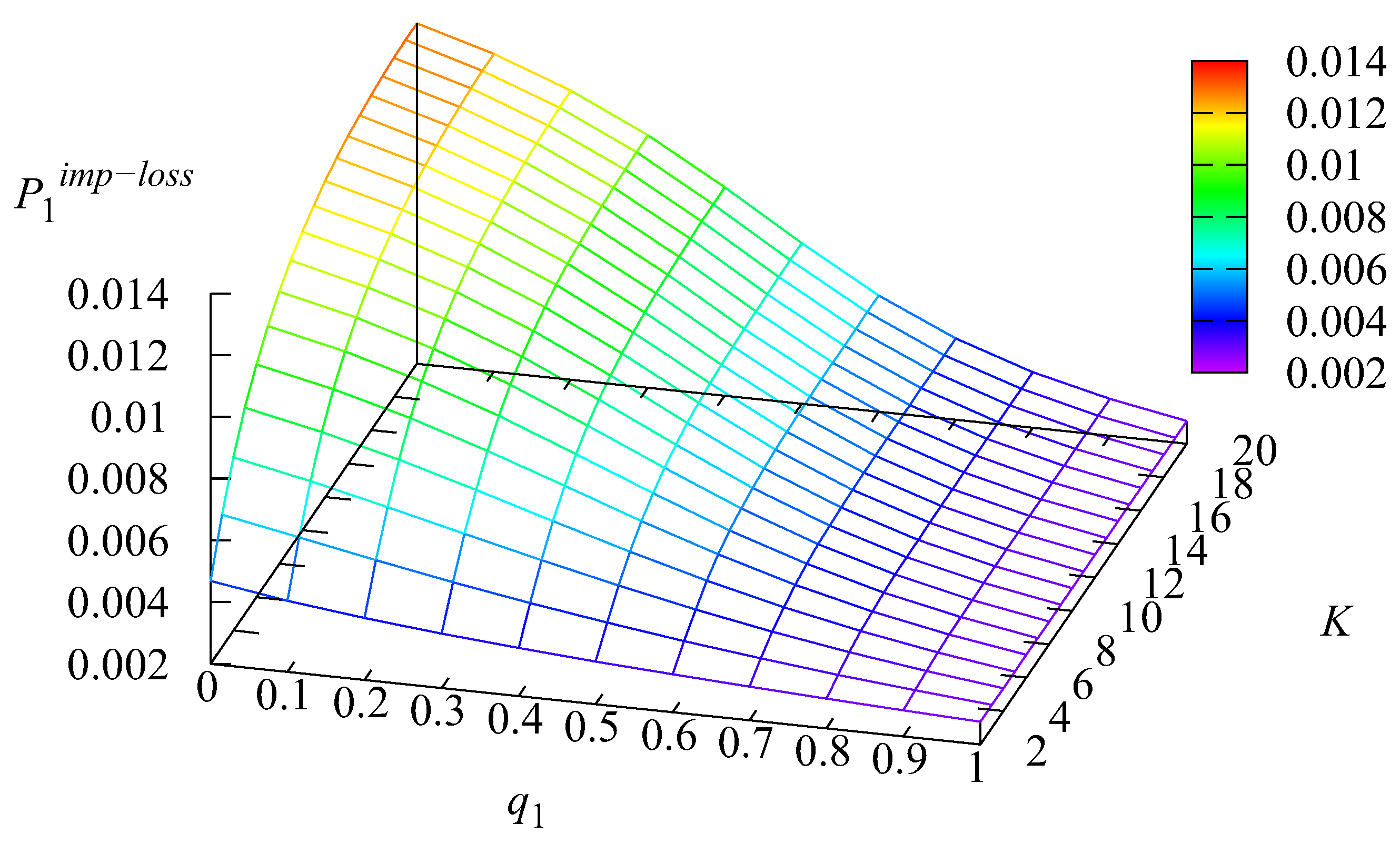
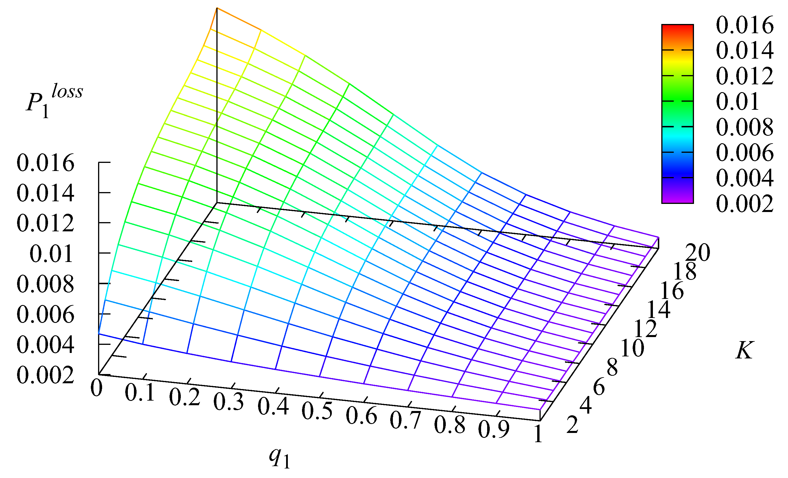
Figure 8 illustrates the dependence of the probability
of an arbitrary type-1 customer loss upon arrival due to Buffer-1 overflow on the parameters
K and
One can see from
Figure 8 that the probability
decreases with an increase in the probability
and increases with a growth in the parameter
K. The maximal value of the probability
is equal to
and is reached for
and
, i.e., when there are type-2 customers in the buffer, type-1 customers are chosen for service only if Buffer-1 is full. The minimal value of this probability is equal to
and is reached for
Note that in the case of
the parameter
K does not impact the system’s operation, and the system’s performance measures do not depend on
K.
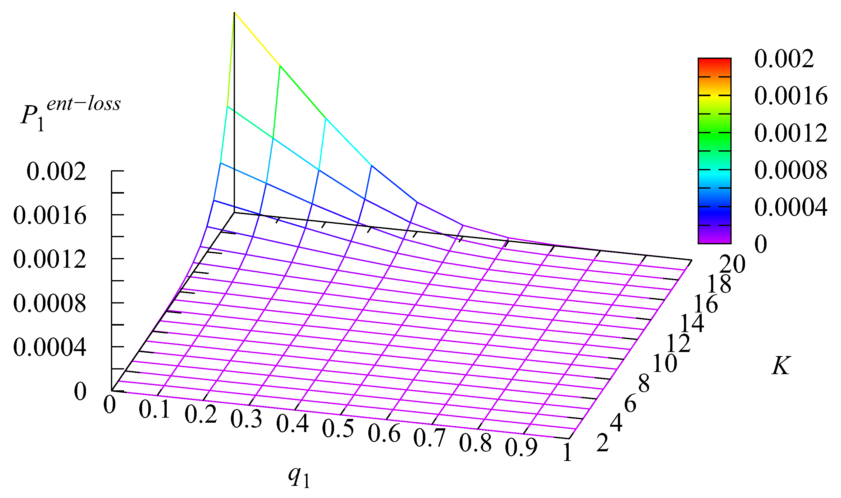
The dependence of the probability
of an arbitrary type-1 customer loss due to impatience in Buffer-1 on the parameters
K and
is presented in
Figure 9.
The probability
also increases with the decrease of the probability
and increases with growth in the parameter
K. The same behavior we can also observe in
Figure 10 that illustrates the dependence of the probability
of an arbitrary type-1 customer loss on the parameters
K and
The loss probability takes its minimal value 0.002738 for This loss mainly occurs due to type-1 customers’ impatience.
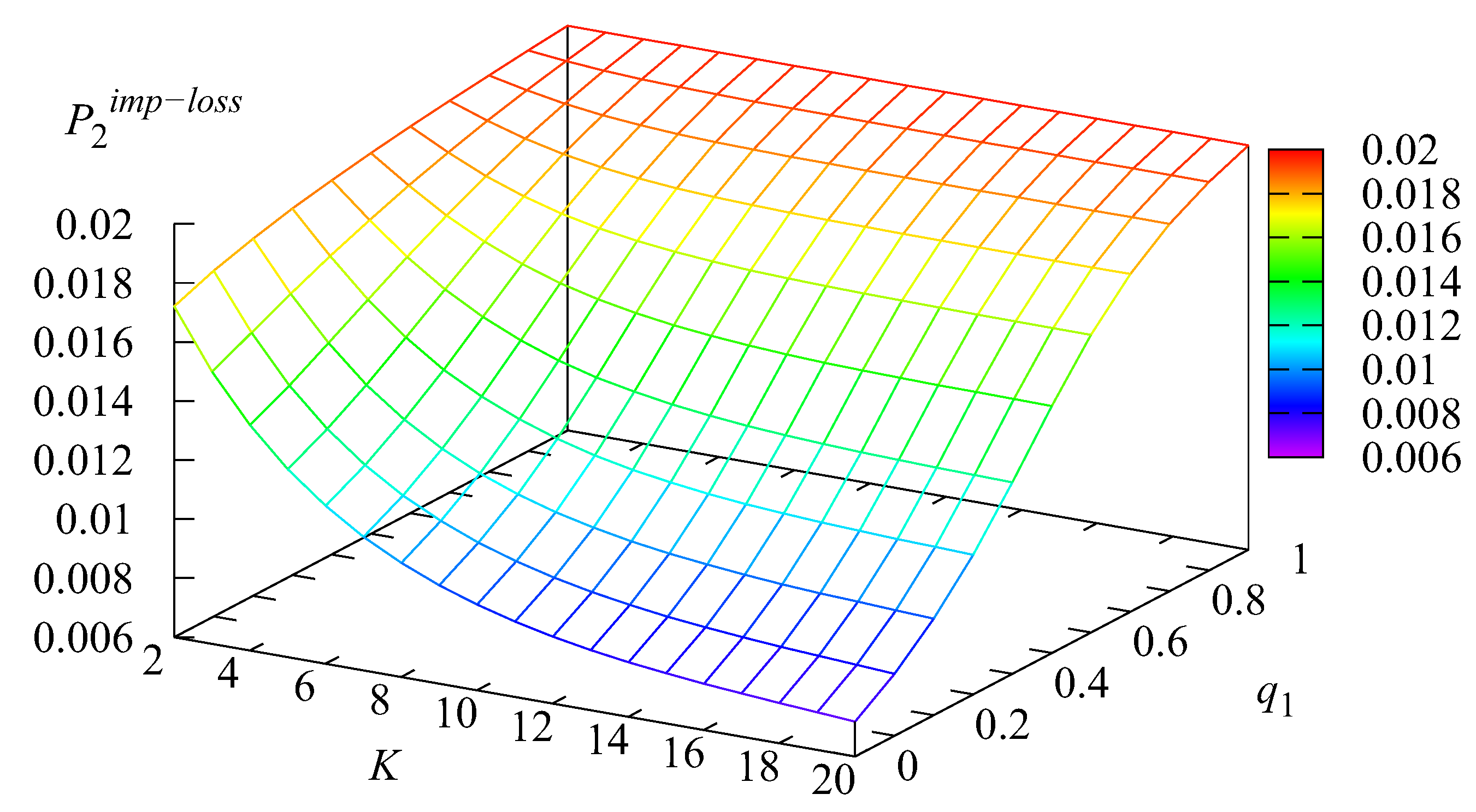
The probability
of an arbitrary type-2 customer loss due to impatience in Buffer-2 behaves oppositely. This probability grows with an increase in the probability
and a decrease in the parameter
K. The shape of the dependence of the probability
on the parameters
K and
is presented in
Figure 11.
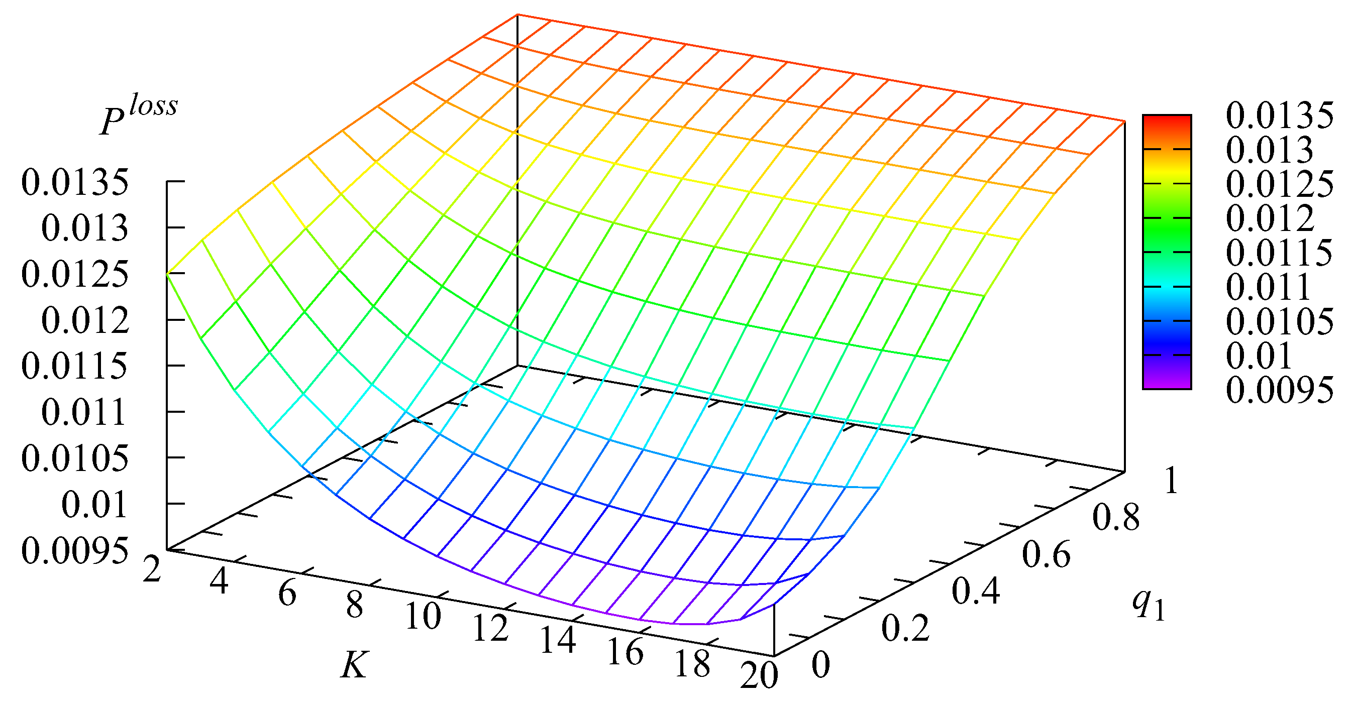
The dependence of the probability
of an arbitrary customer loss on the values
K and
is presented in
Figure 12.
The minimal value of the probability is equal to 0.009641 for and
The quality of system operation can be described by the economic criterion
, which is given in the same way as the criterion from the first experiment. The coefficients
and
also coincide with the cost coefficients from the previous experiment. The dependence of the cost criterion
on the parameters
and
K is presented in
Figure 13.
The economic criterion takes the optimal value for and
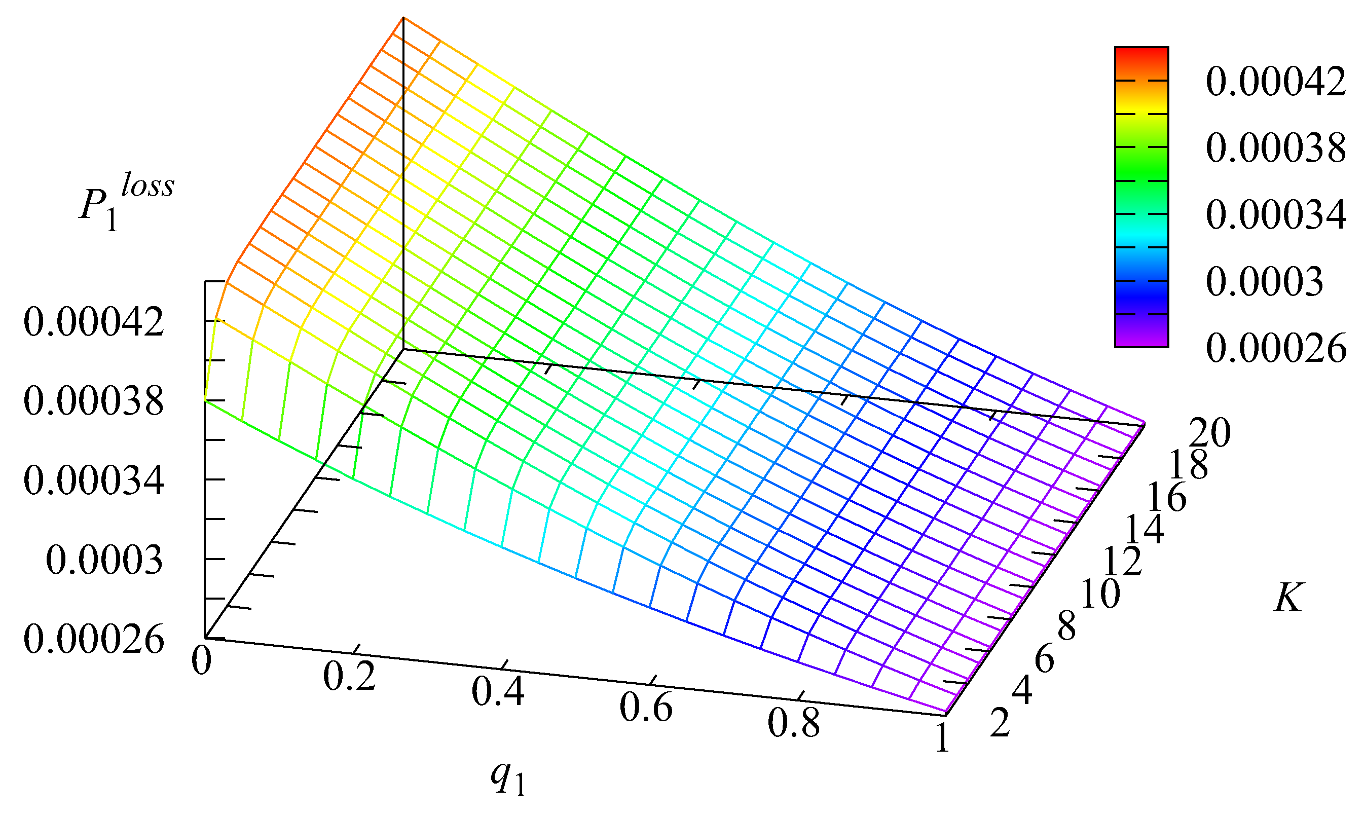
Experiment 3. In the third experiment, instead of a correlated arrival process, we consider two stationary Poisson arrival processes and will show that accounting for only the mean arrival rates and ignoring the correlation and variation of the inter-arrival times can lead to significant errors in assessing the performance of the system under consideration.
Consider the arrival process characterized by the value with the following matrices: It defines a heterogeneous stationary Poisson arrival process with two types of customers having arrival rates and The other parameters coincide with those presented in the second experiment. The control parameters and K are varied in the same way as in the previous experiment.
Figure 14,
Figure 15 and
Figure 16 show the dependence of the probabilities
,
and the cost criterion
E on the parameters
K and
in the case of the heterogeneous stationary Poisson arrival flow.
One can draw the conclusion that the correlation and variance of the arrival process have a significant impact on the systems’ performance indicators by comparing
Figure 10 and
Figure 14,
Figure 11 and
Figure 15, and
Figure 13 and
Figure 16, respectively. If someone tries to evaluate the system with correlated inter-arrival times using the model with the heterogeneous stationary Poisson arrival flow, he/she can obtain huge errors in the estimation. In the case of the heterogeneous stationary Poisson arrival flow, the minimal value of the probability
is equal to 0.000262, while in the case of the
the minimal value of this probability is 0.002738. The minimal value of the probability
is equal to 0.00087 for heterogeneous stationary Poisson arrival flow, while in the case of the
the minimal value of this probability is 0.00717. That means that the real values of the main loss probabilities can be 10 times higher than the values expected based on the model with heterogeneous stationary Poisson arrival flow.
The minimal value of the cost criterion in the case of the heterogeneous stationary Poisson arrival flow is equal to 0.00833988, which is 16 times less than this value for the case of the arrival process.
Therefore, ignorance of positive correlation leads to an overly optimistic prediction of the performance characteristics of the system and an underestimation of the requirements for providing the desired quality of service, such as service rates or the number of servers. This, along with the observation that flows in many real-world systems exhibit correlation and high variability in inter-arrival times, clearly motivates the necessity of analyzing systems with the .


