Constructing Optimal Designs for Order-of-Addition Experiments Using a Hybrid Algorithm

Abstract

For order-of-addition experiments, the response is affected by the addition order of the experimental materials. Consequently, the main interest focuses on creating a predictive model and an optimal design for optimizing the response. Van Nostrand proposed the pairwise-order (PWO) model for detecting PWO effects. Under the PWO model, the full PWO design is optimal under various criteria but is often unaffordable because of the large run size. In this paper, we consider the D-, A- and $M.S.$-optimal fractional PWO designs. We first present some results on information matrices. Then, a flexible and efficient algorithm is given for generating these optimal PWO designs. Numerical simulation shows that the generated design has an appealing efficiency in comparison with the full PWO design, though with only a small fraction of runs. Several comparisons with existing designs illustrate that the generated designs achieve better efficiencies, and the best PWO designs and some selected 100% efficient PWO designs generated by the new algorithm are reported.

1. Introduction

During the past decades, order-of-addition (OofA) experiments have been widely applied to the biochemistry [1] and foot industries [2] as well as chemical-related areas [3] In the mentioned experiments, several components are added into an apparatus sequentially rather than simultaneously, and different addition sequences of reactants yield different responses. However, as the number of components increases, the sample space suffers from a combinatorial explosion, and performing full design becomes unfeasible. Accordingly, our goal is to model for an OofA experiment and construct an informative and economical fractional design.

For the objective of optimizing and predicting the response, several statistical models are created for the OofA experiment: Refs. [4,5,6] proposed a PWO model with diminishing effects for pairwise factors; Ref. [7] added PWO factor interactions to account for sequencing effects not accounted for by pairwise main effects alone; Ref. [8] proposed a component-position (CP) model for order-of-addition using categorical explanatory variables. In this article, we only focus on the first-order PWO model. However, the PWO model is also a regression model. A family of criteria can be applied to find optimal designs under the PWO model, such as D-, A- and $M.S.$-optimal designs. The optimality proof indicates that a full PWO design with $m!$ distinct permutations of components is D-, A-, and $M.S.$-optimal, but the run size is extremely large. Taking $m=10$ as an example, there are $m!=3,628,800$ distinct permutations. Consequently, over three million runs of experiments should be implemented, which is impractical. Therefore, fractions of full PWO designs with a smaller number of runs are preferable.

Recently, four kinds of fractional PWO designs have been studied. Ref. [4] introduced a method for constructing optimal PWO designs. This method limits the run size to $m!/r!(2\le r\le m/2)$, which is also too many for experimenters to afford. For instance, if $m=10$, the method needs at least 30,240 runs to be implemented. Refs. [8,9] provided construction methods based on an orthogonal array; the resulting designs are component orthogonal arrays (COAs) and OofA orthogonal arrays (OofA-OAs), in which the run size is also inflexible. Ref. [10] provided a minimal-point design with $m(m-1)/2+1$ runs. The run size is small, but the efficiency is relatively low. However, theoretical constructions of these fractional PWO designs are highly dependent on run size. Ref. [11] applied the threshold-accepting algorithm to construct the optimal designs (D-efficiency for application) based on the pairwise-order (PWO) model and the tapered PWO model; the designs obtained by threshold-accepting algorithm for $4\le m\le 30$ with $n=m(m-1)/2+1,m(m-1)+1,3m(m-1)/2+1,$ respectively, are provided for practical uses.

This article gives serious consideration to constructing D-, A-, and $M.S.$-optimal PWO designs. The main contributions of this article are as follows. First, we construct a new hybrid algorithm for generating the PWO design, which is flexible with no restriction on run size. Second, D-, A-, and $M.S.$-optimal PWO designs can be constructed using the proposed algorithm. Third, the constructed designs possess high efficiencies compared with the full PWO design, though with a small fraction of runs. Some optimal PWO designs and fully efficient PWO designs are listed in the tables.

This paper is organized as follows. We first introduce the PWO model in Section 2. Section 3 gives a review of Fedorov’s exchange algorithm for constructing the D-optimal designs. Then, this algorithm is modified and extended for constructing A- and $M.S.$-optimal designs. Some theoretical results on the information matrix and algorithm are also provided in Section 3. In Section 4, based on the exchange algorithm and particle swarm optimization (PSO) algorithm, a novel hybrid algorithm is proposed to achieve D-, A- and $M.S.$-optimal PWO designs. Some numerical results are given in Section 5. Finally, concluding remarks are provided in Section 6.

2. Model Specification

Now, we introduce the Van Nostrand PWO model. Suppose there are m components denoted as $1,\dots ,m$. Any treatment in the OofA experiment corresponds to a permutation of $1,\dots ,m$, denoted as $\alpha$, and the first-order PWO model can be expressed as follow

$$\tau (\alpha )={\beta }_0+\sum _{1\le j<k\le m}{z}_{jk}(\alpha ){\beta }_{jk},$$

where each $z_{jk}(\alpha )$ is a PWO indicator between j and k,

$$z_{jk}(\alpha )=\left\{\begin{array}{cc}1\hfill & \mathrm{if}j\mathrm{precedes}k\mathrm{in}\alpha ,\hfill \\ -1\hfill & \mathrm{if}k\mathrm{precedes}j\mathrm{in}\alpha .\hfill \end{array}\right.$$

(1)

For an n-point PWO design, let Y be the n-dimensional response vector, Z be the design matrix with $\left(\genfrac{}{}{0pt}{}{m}{2}\right)$ columns corresponding to PWO indicators $z_{12},z_{13},\dots ,z_{(m-1)m}$, and $\beta =({\beta }_{12},{\beta }_{13},\dots ,$ ${\beta }_{(m-1)m}{)}^{\prime }$, where ${}^{\prime }$ denotes the transpose. Then, the first-order PWO model can be written as

$$Y=\mathbf{1}{\beta }_0+Z\beta +ϵ,$$

(2)

or

$$Y=X\tilde{\beta }+ϵ,$$

(3)

where $X={(\mathbf{1}Z)}_{n\times p}$ with $p=\left(\genfrac{}{}{0pt}{}{m}{2}\right)+1$ is the model matrix, $\tilde{\beta }={({\beta }_0,{\beta }^{\prime })}^{\prime }$ represents the parameter of interest, and the random error $ϵ\sim N(\mathbf{0},{\sigma }^{2}I)$. Ref. [7] extended the PWO model to the high-order case. Here, we only consider a first-order PWO model. The proposed algorithms also apply to a higher-order PWO model.

Furthermore, we refer to $\tilde{M}=X^{\prime }X/n$ as the information matrix of an n-point PWO design. Under the PWO model (3), the variance-covariance matrix of the least squares estimator of $\beta$ is proportional to $\tilde{M}$. Hence, it is desirable to maximize the matrix $\tilde{M}$ under some criteria. The popular criteria include the D-criterion $det{(\tilde{M})}^{1/p}$, the A-criterion $tr({\tilde{M}}^{-1})$, the $M.S.$-criterion $tr({\tilde{M}}^2)$ (see the reference [12]). Note that $tr({\tilde{M}}^{-1})$ is interpreted as $+\infty$ for singular $X^{\prime }X$. Let $X_f$ be the full PWO design and the corresponding information matrix be ${\tilde{M}}_f=X_f^{\prime }{X}_f/n$. For clarity, we take $m=3$ as an example to illustrate the characteristics of the full PWO design under D-, A- and $M.S.$-criteria. The levels of PWO factors in the full PWO design with three components are as follows

Table 1. Full PWO design with 3 components.

Run	Order-of-Addition	${\mathit{z}}_{12},{\mathit{z}}_{13},{\mathit{z}}_{23}$
1	1 2 3	1, 1, 1
2	1 3 2	1, 1, −1
3	2 1 3	−1, 1, 1
4	2 3 1	−1, −1, 1
5	3 1 2	1, −1−1
6	3 2 1	−1, −1, −1

.

From this table, table we obtain

$$X_f=\left(\begin{array}{cccc}\hfill 1& \hfill 1& \hfill 1& \hfill 1\\ \hfill 1& \hfill 1& \hfill 1& \hfill -1\\ \hfill 1& \hfill -1& \hfill 1& \hfill 1\\ \hfill 1& \hfill -1& \hfill -1& \hfill 1\\ \hfill 1& \hfill 1& \hfill -1& \hfill -1\\ \hfill 1& \hfill -1& \hfill -1& \hfill -1\end{array}\right),{\tilde{M}}_f=\left(\begin{array}{cccc}\hfill 1& \hfill 0& \hfill 0& \hfill 0\\ \hfill 0& \hfill 1& \hfill 1/3& \hfill -1/3\\ \hfill 0& \hfill 1/3& \hfill 1& \hfill 1/3\\ \hfill 0& \hfill -1/3& \hfill 1/3& \hfill 1\end{array}\right),$$

and $det({\tilde{M}}_f)=16/27,$ $tr({\tilde{M}}_f^{-1})=11/2$ and $tr({\tilde{M}}_f^2)=14/3$.

3. Exchange Algorithms for Constructing $\mathit{D}$-, $\mathit{A}$-, and $\mathit{M}.\mathit{S}.$-Optimal Designs

Theoretical constructions on optimal designs are always complicated; hence, computer algorithms are applied for constructing approximate and exact optimal designs in the literature. The exchange algorithm is one of the popular computer algorithms for constructing optimal designs for the cases with the design points being selected from a finite design space. [13] first proposed an exchange algorithm for generating D-optimal designs. This algorithm chooses n points to include in the design from a finite set of possible points called candidate points. It starts with nonsingular n-point designs and then adds and deletes one observation to achieve increases in the determinant. After that, some improved implementations are proposed based upon Fedorov’s exchange algorithm, such as the Kiefer round-off algorithm, the Mitchell algorithm, the Wan Schalkwyk algorithm, the combined Fedorov, the Wynn–Mitchell algorithm, and so on; see the references [14,15].

3.1. The Single-Point Exchange Procedure

Consider an n-point design $D={\left\{{\alpha }_i\right\}}_{i=1}^n$ under model (3), with a corresponding model matrix $X={(x_1,\dots ,x_n)}^{\prime }$. If $\tilde{M}=X^{\prime }X/n$, then the D-, A- and $M.S.$-criteria maximize $det{(\tilde{M})}^{1/p},$ $-tr({\tilde{M}}^{-1})$ and $-tr({\tilde{M}}^2)$, respectively, which are equivalent to maximizing $\varphi (D)=det(M),-tr(M^{-1})$ and $-tr(M^2)$, respectively, where $M=X^{\prime }X={\sum }_{i=1}^n{x}_i{x}_i^{\prime }$.

Inspired by Fedorov’s exchange algorithm, we develop a new exchange algorithm for generating D-, A- and $M.S.$-optimal designs simultaneously. This algorithm is realized by multiple iterations of the single-point exchange procedure which works as follows.

Single-point exchange procedure: 

Let X be the model matrix of the original design and $M=X^{\prime }X.$

(1) 

Find a vector x among the vectors of the complementary design such that $u(x)$ is maximum and add x to the current n-point design;

(2) 

Find a vector $x_i$ among the $n+1$ vectors of the current $n+1$-point design such that $v(x_i)$ is minimum and remove $x_i.$

When using the single-point exchange procedure for generating the D-, A- and $M.S.$-optimal designs, the objective functions are denoted as $u_{*}(x)$ and $v_{*}(x_i)$ with $\ast =D,A,M.S.$ and defined as below:

$$u_D(x)=x^{\prime }{M}^{-1}x,v_D(x_i)=x_i^{\prime }{M}_x^{-1}{x}_i;$$

(4)

$$u_A(x)=\frac{x^{\prime }{M}^{-2}x}{1+x^{\prime }{M}^{-1}x},v_A(x)=\frac{x_i^{\prime }{M}_x^{-2}{x}_i}{1-x_i^{\prime }{M}_x^{-1}{x}_i};$$

(5)

$$u_{M.S.}(x)=-x^{\prime }Mx,v_{M.S.}(x_i)=-x_i^{\prime }{M}_x{x}_i;$$

(6)

where $M={\sum }_{i=1}^n{x}_i{x}_i^{\prime }$ is the moment matrix of the current design and M is updated to $M_x=M+x{x}^{\prime }$ when a candidate point from the complementary design is added to the current design.

Here, the complementary design consists of all candidate points from the design space except for the n points of the current design.

Theorem 1. 

For D-, A-, and $M.S.$-criteria which maximize $\varphi (D)=det(M),-tr(M^{-1})$ and $-tr(M^2)$, respectively, the design generated by the single-point procedure with $u(x)$ and $v(x_i)$ defined as Equations (4)–(6) leads to no decrease in $\varphi (D).$

The proof of this theorem uses some matrix theories, and we present it in the Appendix A. This theorem implies that the exchange algorithm will return local D-, A- and $M.S.$-optimal designs over multiple iterations of the single-point exchange procedure.

3.2. The Technique for Avoiding the Singularity of the Matrix for the Exchange Algorithm

For generating optimal design using a computer search algorithm, the solution is often trapped into the local optimal design. Thus random exchange method is always used to avoid this drawback. For constructing D-, A- and $M.S.$-optimal designs using a computer search algorithm, a randomly selected initial design possibly corresponds to a singular moment matrix, a and computation problem then arises. This is a significant issue, especially for the case with a rather small number of n. Take the case with $n=\left(\genfrac{}{}{0pt}{}{m}{2}\right)+1(m=4,5)$ as an example. Among all $\left(\genfrac{}{}{0pt}{}{m!}{n}\right)$ options of n-point design, a large proportion of them correspond to a badly conditioned matrix M. As shown in Figure 1, all the reciprocal condition numbers are near 0, and the reciprocal condition number below ${10}^{-12}$ is counted in the first bin of each histogram with a probability exceeding $50\%$.

A randomly selected initial design will return a computationally singular matrix M with a large probability. For this reason, we address the issue of avoiding singularities of M and $M_x$ in the single-point exchange algorithm. Two types of techniques are provided regarding this issue. The first technique is to start with a nonsingular design instead of starting with a randomly selected design.

Remark 1. 

If the initial design has a nonsingular moment matrix, then by $M_x=\left|M\right|(1+x^{\prime }{M}^{-1}x)$ and $M_x-x_i{x}_i^{\prime }=\left|M_x\right|(1-x_i^{\prime }{M}_x^{-1}{x}_i)$, where $x_i^{\prime }{M}_x^{-1}{x}_i\le x^{\prime }{M}_x^{-1}x=\frac{x^{\prime }{M}^{-1}x}{1+x^{\prime }{M}^{-1}x}<1$, both $M_x$ and $M_x-x_i{x}_i^{\prime }$ are nonsingular matrices during each iteration of the single-point exchange algorithm which is performed recursively.

This technique is practical since a nonsingular initial design with n points can be obtained by appending $n-\left(\genfrac{}{}{0pt}{}{m}{2}\right)-1$ randomly selected distinct points to the minimal-point design provided in [10]. However, in the hybrid algorithm, the design is updated via both the single-point exchange procedure and some random exchange procedure.

The second technique is inspired by the DETMAX algorithm in [14], a specified nonsingular matrix multiplied by a very small positive parameter $\theta$ is added to matrix M or $M_x$. Taking M as an example, we do not consider $M^{-1}$ directly, but instead attempt to calculate ${(M+\theta (X_f^{\prime }{X}_f/N_f))}^{-1}$, where $N_f$ is the number of candidate points, and $X_f$ is the model matrix of the full design composed of all $N_f$ candidate points. Then, one technique that we can use to avoid the singularity of the matrix is as follows.

Remark 2. 

To avoid singularity, $x^{\prime }{(M+\theta (X_f^{\prime }{X}_f/N_f))}^{-1}x$ and $x_i^{\prime }{(M_x+\theta (X_f^{\prime }{X}_f/N_f))}^{-1}{x}_i$ are maximized and minimized in the single-point exchange algorithm with $u(x)$ and $v(x_i)$ being defined as Equations (4) and (5). The degree of error involved in considering these alternative matrices is less than θ.

To appreciate the degree of error involved in considering the alternative matrix, one can make the following calculations. Let

$$f(\theta )=x^{\prime }{(M+\theta (X_f^{\prime }{X}_f/N_f))}^{-1}x.$$

Then, apply the technique in Mitchell (2000) to extend $f(\theta )$ in a Taylor series about $\theta =0$ to obtain the linear approximation:

$$\begin{array}{ccc}\hfill f(\theta )& \cong & f(0)+\theta \left(\frac{df(\theta )}{d\theta }\right){|}_{\theta =0}\hfill \\ & =& x^{\prime }{M}^{-1}x-\theta \left(x^{\prime }{(M+\theta (X_f^{\prime }{X}_f/N_f))}^{-1}(X_f^{\prime }{X}_f)/N_f{(M+\theta (X_f^{\prime }{X}_f/N_f))}^{-1}x\right){|}_{\theta =0}\hfill \\ & =& x^{\prime }{M}^{-1}x-\theta x^{\prime }{M}^{-1}{X}_f^{\prime }{X}_f{M}^{-1}x/N_f.\hfill \end{array}$$

For small $\theta$, the error in considering $x^{\prime }{(M+\theta (X_f^{\prime }{X}_f/N_f))}^{-1}x$ instead of $x^{\prime }{M}^{-1}x$ is nearly $\theta x^{\prime }{M}^{-1}{X}_f^{\prime }{X}_f{M}^{-1}x/N_f$. In the proposed algorithm, the value of $\theta$ is set at 0.005, which is found to be quite satisfactory in simulations. This choice based on the run size of the full PWO is sufficiently large such that $x^{\prime }{M}^{-1}{X}_f^{\prime }{X}_f{M}^{-1}x/N_f<1$, and the error will be less than $0.5\%$.

Note that in this paper, we adopt the technique described in Remark 2 to avoid the singularity of the matrix.

3.3. The Performance of the Exchange Algorithm

Now, we discuss the performance of the exchange algorithm. The single-point exchange procedure is performed recursively, and the D-, A- and $M.S.$-efficiencies of the generated designs are calculated. For brevity, the cases with $m=4,5,6,7$ components are considered and the run sizes are fixed at $n=m(m-1)$. The following Figure 2 shows that the efficiencies are deeply increased in former iterations but then stabilized and slow on one value as the number of iterations increased. Therefore, the exchange algorithm yields locally optimal designs that approximate a global optimal design in a reasonable number of iterations.

To illustrate the performance of the exchange algorithm for constructing D-, A- and $M.S.$-optimal designs, 1000 designs are generated by the exchange algorithm concerning each pair of the objective functions defined in Equations (4)–(6). The initial designs are randomly selected. We list the minimum, average, and maximum efficiencies of the generated designs in

Table 2. Efficiencies of 1000 designs generated by the exchange algorithm.

		D-Efficiency			A-Efficiency			$\mathit{M}.\mathit{S}.$-Efficiency
m	Runs	Min	Ave	Max	Min	Ave	Max	Min	Ave	Max
4	12	97.4%	99.8%	100%	32.1%	65.3%	92.4%	76.3%	97.7%	100%
5	20	94.2%	96.0%	97.0%	19.5%	51.7%	73.9%	74.4%	96.5%	98.2%
6	30	93.8%	95.8%	97.1%	19.1%	48.0%	69.5%	95.2%	96.8%	98.1%
7	42	93.7%	95.3%	96.7%	33.4%	47.7%	63.4%	95.9%	97.1%	98.0%

. The generated designs are largely depended on the initial designs, most of them are locally optimal designs and some of them even have lower efficiencies than 80%; see the numbers in bold font. Thus, in the next section, we propose a more robust hybrid algorithm that combines the exchange algorithm and the particle swarm algorithm to produce approximate optimal designs with higher efficiency than designs generated by the exchange algorithm.

4. Constructions on $\mathit{D}$-, $\mathit{A}$- and $\mathit{M}.\mathit{S}.$-Optimal PWO Designs Using a Hybrid Algorithm Combining the Exchange Algorithm and PSO Algorithm

Before introducing the new algorithm, we add some details of the PSO algorithm. PSO is a population-based stochastic algorithm for optimization. Each population member is described as a particle that moves around a search space testing new criterion values. All particles survive from the beginning of a trial until the end, and their interactions result in iterative improvement of the quality of the problem solutions over time. The most common type of implementation defines the particles’ behavior as adjusting toward each of its personal best position (local-best) and global-best position so that its trajectory shifts to new regions of the search space and the particles gradually cluster around the optima. To generate optimal experimental designs, a particularly challenging task is to redefine the particle designs’ movement toward its personal local-best design and global-best design. A review of some recent applications of PSO and its variants to tackle various types of efficient experimental design is [16]. Since finding optimal PWO designs for the OofA experiment is to solve a discrete optimization problem, we utilize an update procedure for the particle designs that is similar to the modified PSO algorithms in [17,18]. Each particle design relates to its personal local-best design which is derived by exchange procedures starting from itself. During each iteration, the current particle design is adjusted toward its personal local-best design as well as the global-best design by exchanging points with each other.

Now, we introduce a new hybrid algorithm called Ex-PSO algorithm, which combines the single-point exchange algorithm and PSO algorithm for generating D-, A-, and $M.S.$-optimal designs. The single-point exchange algorithm is used for generating the local-best design concerning each particle design. The PSO algorithm ensures the particle designs gradually cluster around the optimal PWO design. To avoid singularity, the technique proposed in Remark 2 is used; hence, a parameter $\theta$ with a small value is involved in this algorithm.

Since the Ex-PSO algorithm involves a set of parameters denoted as $s,t_{ex},t_{pso},\theta ,c_1,c_2$, we also refer to it as Ex-PSO $(m,n;s,t_{ex},t_{pso},\theta ,c_1,c_2)$ for generating optimal PWO design with m components and n runs. For clarity, we create a programming chart to illustrate the steps of Ex-PSO $(m,n;s,t_{ex},t_{pso},\theta ,c_1,c_2)$. Further, we explain the optimization process and the uses of these parameters as follows. Denote ${\mathcal{L}}_k$s and $\mathcal{G}$ as the local-best designs and the global-best design, respectively. These designs are updated during each iteration of the Ex-PSO algorithm. Each local-best design ${\mathcal{L}}_k$ is derived from the current particle design $D_k$ via a fixed number of iterations of the single-point exchange procedure, denoted as $t_{ex}$. In addition, the global-best design $\mathcal{G}$ is the optimal local-best design that maximizes $\varphi ({\mathcal{L}}_k)$. The number of iterations of the PSO algorithm is denoted as $t_{pso}$. Meanwhile, two parameters are used to control the PSO behavior of the Ex-PSO algorithm: $c_1$ and $c_2$, which account for the velocities at which each current design drifts toward the corresponding local-best and global-best design. More specifically, during each iteration of the PSO algorithm, we randomly exchange $c_1$ points from the difference set $D_k\setminus {\mathcal{L}}_k$ with $c_1$ points from ${\mathcal{L}}_k\setminus D_k$ and then randomly exchange $c_2$ points from the difference set $D_k\setminus \mathcal{G}$ with $c_2$ points from $\mathcal{G}\setminus D_k$. This procedure corresponds to the “Update $D_k$ by PSO" box in the programming chart.

Finally, we note that the time complexity for each iteration is $O(n^3)$. However, the search procedure of PSO also relates to the full design which is a combinatorial large set with $m!$ points, so Ex-PSO algorithm may be time-consuming for large m. The Ex-PSO algorithm (Algorithm 1) implemented in MATLAB running on Intel(R) Core(TM) i7-8550U GHz with 8 GB Memory. Take the case of $m=6,n=16$ for example; it takes 30.42 seconds for running Ex-PSO $(6,16;10,20,100,0.005,1,1)$.

Algorithm 1 Ex-PSO $(m,n;s,t_{ex},t_{pso},\theta ,c_1,c_2)$

1: Randomly initialize $D_k,k=1,\dots ,s$. 2: Calculate $\varphi (D_k),k=1,\dots ,s$. 3: Initial ${\mathcal{L}}_k\leftarrow D_k,k=1,\dots ,s$ and $\mathcal{G}\leftarrow argma{x}_{1\le k\le s}\varphi ({\mathcal{L}}_k)$ 4: for $i=1$ to $t_{pso}$ do 5:    Update each $D_k$ by single-point exchange procedure 6:    Calculate $\varphi (D_k),k=1,\dots ,s$ 7:    if $\varphi (D_k)>\varphi ({\mathcal{L}}_k)$ then 8:      Update ${\mathcal{L}}_k$ by $D_k$ 9:    end if 10:    if $\varphi ({\mathcal{L}}_k)>\varphi (\mathcal{G})$ then 11:      Update $\mathcal{G}$ by ${\mathcal{L}}_k$ 12:    end if 13: end for 14: return $\mathcal{G}$

5. Numerical Simulations

In this section, we illustrate the performances of the obtained designs constructed by Algorithm 1. For brevity, the generated designs are denoted as Ex-PSO-D, Ex-PSO-D and Ex-PSO-M.S. designs that respectively correspond to the objective functions (4)–(6) which are considered in the exchange algorithm. Numerical simulations show that these designs are powerful for fitting PWO models in terms of the D-, A- and $M.S.$-efficiencies. The efficiencies are derived from comparison with the full PWO design since the information matrix of the full PWO design has been proven to be universally optimal. Therefore, we have the D-, A- and $M.S.$-efficiencies that calculate $\frac{det{(\tilde{M})}^{1/p}}{det{({\tilde{M}}_f)}^{1/p}}$, $\frac{tr({\tilde{M}}_f^{-1})}{tr({\tilde{M}}^{-1})}$ and $\frac{tr({\tilde{M}}_f^2)}{tr({\tilde{M}}^2)}$, respectively, where $\tilde{M}$ and ${\tilde{M}}_f$ are the information matrices of the obtained design and full PWO design, respectively, and p is the number of the columns of the model matrix X.

The number of PSO particles (s), the maximum iteration counts of the single-point exchange algorithm and PSO algorithm ($t_{ex},t_{pso}$), and the numbers of pairs of exchanging points with which each particle design drifts toward the local-best and global-best design $(c_1,c_2)$, control the optimization process of Ex-PSO algorithm. It seems reasonable that these parameters should be increased for large n and m. In our test of searching for optimal PWO designs with $m=4,5,6,7$ components, we recommend that these parameters be set at $s=10$, $t_{ex}=20$, $t_{pso}=100$, $c_1=c_2=1$. Furthermore, we recommend setting the maximum iteration counts of the exchange algorithm and PSO at $t_{ex}=20$ and $t_{pso}=100$, respectively, which achieves high computational efficiency. Further, to demonstrate the performance of such a set of parameters, we randomly run the algorithm Ex-PSO $(m,n;10,20,100,0.005,1,1)$ one hundred times for generating the Ex-PSO-D designs, because the exchange algorithm seems inefficient under A-optimal criterion, as shown in Figure 3. Therefore, one hundred Ex-PSO-D designs with $m=4,5,6,7$ components and $n=m(m-1)$ runs are generated, and

Table 3. An Ex-PSO-D design with 4 components and 12 runs.

Run	Order-of-Addition	${\mathit{z}}_{12},{\mathit{z}}_{13},{\mathit{z}}_{14},{\mathit{z}}_{23},{\mathit{z}}_{24},{\mathit{z}}_{34}$
1	1 4 2 3	1, 1, 1, 1, −1, −1
2	1 2 4 3	1, 1, 1, 1, 1, −1
3	1 3 2 4	1, 1, 1, −1, 1, 1
4	2 1 3 4	−1, 1, 1, 1, 1, 1
5	2 4 3 1	−1, −1, −1, 1, 1, −1
6	2 3 4 1	−1, −1, −1, 1, 1, 1
7	3 1 4 2	1, −1, 1, −1, −1, 1
8	3 2 1 4	−1, −1, 1, −1, 1, 1
9	3 4 1 2	1, −1, −1, −1, −1, 1
10	4 1 3 2	1, 1, −1, −1, −1, −1
11	4 2 1 3	−1, 1, −1, 1, −1, −1
12	4 3 2 1	−1, −1, −1, −1, −1, −1

highlights that all Ex-PSO-D designs reach at least $93\%$ of the efficiency of the full PWO design. For the cases with large m, the settings on maximum iterations, $t_{ex}$ and $t_{pso}$ may not be enough, but the Ex-PSO algorithm still returns approximate optimal PWO designs; see

Table 4. Comparison of $det{(\tilde{M})}^{1/p}$ and D-efficiency of PWO designs.

m	n	${\mathit{D}}_{\mathbf{peng}}$	${\mathit{D}}_{\mathbf{coa}}$	${\mathit{D}}_{\mathbf{ta}}$	${\mathit{D}}_{\mathbf{ex}}$	${\mathit{D}}_{\mathbf{ex}-\mathbf{pso}}$
4	7	-	-	0.6966 (89.6%)	0.6966 (89.6%)	0.6966 (89.6%)
	12	0.7773 (100%)	0.7064 (90.9%)	0.7773 (100%)	0.7773 (100%)	0.7773 (100%)
5	11	-	-	0.6379 (90.3%)	0.6211 (87.9%)	0.6379 (90.3%)
	20	-	0.6354 (89.9%)	0.6855 (97.0%)	0.6840 (96.8%)	0.6855 (97.0%)
	60	0.7067 (100%)	-	0.7067 (100%)	0.7061 (99.9%)	0.7067 (100%)
6	16	-	-	0.5778 (88.1%)	0.5612 (85.6%)	0.6002 (91.5%)
	30	-	0.5710 (87.1%)	0.6344 (96.7%)	0.6372 (97.2%)	0.6381 (97.3%)
	120	0.6558 (100%)	-	0.6552 (99.9%)	0.6555 (99.95%)	0.6558 (100%)
7	22	-	-	0.5016 (81.2%)	0.5325 (86.2%)	0.5409 (87.6%)
	42	-	0.5800 (93.9%)	0.5958 (96.4%)	0.5996 (97.0%)	0.5998 (97.1%)
	840	0.6178 (100%)	-	0.6178 (100%)	0.6177 (99.99%)	0.6178 (100%)

,

Table 5. Comparison of $tr({\tilde{M}}^{-1})$ and A-efficiency of PWO designs.

m	n	${\mathit{D}}_{\mathbf{peng}}$	${\mathit{D}}_{\mathbf{coa}}$	${\mathit{D}}_{\mathbf{ta}}$	${\mathit{D}}_{\mathbf{ex}}$	${\mathit{D}}_{\mathbf{ex}-\mathbf{pso}}$
4	7	-	-	17.5000 (67.4%)	-	14.8750 (79.3%)
	12	11.8000 (100%)	14.5000 (81.4%)	11.8000 (100%)	11.8000 (100%)	11.8000 (100%)
5	11	-	-	28.2898 (74.2%)	-	26.4773 (79.3%)
	20	-	26.0000 (80.8%)	22.4550 (93.5%)	22.3910 (93.8%)	22.3311 (94.0%)
	60	21.0000 (100%)	-	21.0337 (99.8%)	21.0000 (100%)	21.0000 (100%)
6	16	-	-	46.0558 (72.0%)	-	40.8428 (81.2%)
	30	-	45.3736 (73.0%)	35.3203 (93.8%)	35.0989 (94.4%)	35.0144 (94.7%)
	120	33.1429 (100%)	-	33.2443 (99.7%)	33.2023 (99.8%)	33.1721 (99.9%)
7	22	-	-	76.4729 (63.1%)	-	72.4088 (66.6%)
	42	-	57.1177 (84.5%)	51.6845 (93.4%)	51.0578 (94.5%)	51.5024 (93.7%)
	840	48.2500 (100%)	-	48.2583 (99.98%)	48.2738 (99.95%)	48.2555 (99.99%)

Note: $D_{ex}$ with $n=m(m-1)/2+1$ is omitted because it reports an error of “singular design". When running the optFederov function from the AlgDesign package in R.

and

Table 6. Comparison of $tr({\tilde{M}}^2)$ and $M.S.$-efficiency of PWO designs.

m	n	${\mathit{D}}_{\mathbf{peng}}$	${\mathit{D}}_{\mathbf{coa}}$	${\mathit{D}}_{\mathbf{ta}}$	${\mathit{D}}_{\mathbf{ex}-\mathbf{pso}}$
4	7	-	-	10.4694 (92.3%)	10.4694 (92.3%)
	12	9.6667 (100%)	10.3333 (93.6%)	9.6667 (100%)	9.6667 (100%)
5	11	-	-	18.5207 (95.4%)	18.5207 (95.4%)
	20	-	19.0000 (93.0%)	18.0400 (97.9%)	18.0000 (98.2%)
	60	17.6667 (100%)	-	17.6667 (100%)	17.6667 (100%)
6	16	-	-	31.0000 (94.6%)	30.9688 (94.7%)
	30	-	31.3333 (93.6%)	29.8756 (98.2%)	29.8311 (98.3%)
	120	29.3333 (100%)	-	29.3556 (99.92%)	29.3733 (99.89%)
7	22	-	-	47.5702 (95.3%)	47.7686 (94.9%)
	42	-	45.8095 (99.0%)	45.9048 (98.8%)	46.1905 (98.1%)
	840	45.3333 (100%)	-	45.3349 (99.99%)	45.3368 (99.99%)

in the following part.

To illustrate the advantages of the obtained designs for fitting PWO model, we compare the Ex-PSO-D designs for four components and 12 runs with the optimal PWO design in [4].

Example 1. 

The following is a Ex-PSO-D design with 4 components and 12 runs generated by Ex-PSO $(4,12;10,20,100,0.005,1,1).$

The information matrix of this design under the first-order PWO model is

$$\tilde{M}=\left(\begin{array}{ccccccc}\hfill 1& \hfill 0& \hfill 0& \hfill 0& \hfill 0& \hfill 0& \hfill 0\\ \hfill 0& \hfill 1& \hfill 1/3& \hfill 1/3& \hfill -1/3& \hfill -1/3& \hfill 0\\ \hfill 0& \hfill 1/3& \hfill 1& \hfill 1/3& \hfill 1/3& \hfill 0& \hfill -1/3\\ \hfill 0& \hfill 1/3& \hfill 1/3& \hfill 1& \hfill 0& \hfill 1/3& \hfill 1/3\\ \hfill 0& \hfill -1/3& \hfill 1/3& \hfill 0& \hfill 1& \hfill 1/3& \hfill -1/3\\ \hfill 0& \hfill -1/3& \hfill 0& \hfill 1/3& \hfill 1/3& \hfill 1& \hfill 1/3\\ \hfill 0& \hfill 0& \hfill -1/3& \hfill 1/3& \hfill -1/3& \hfill 1/3& \hfill 1\end{array}\right).$$

If the rows are rearranged, this design is the same as the optimal PWO design with $4!/2!$ runs constructed by [4]. This design also features projective properties [6]. All 4 subsets of three components correspond to two-times-replicated three-component designs.

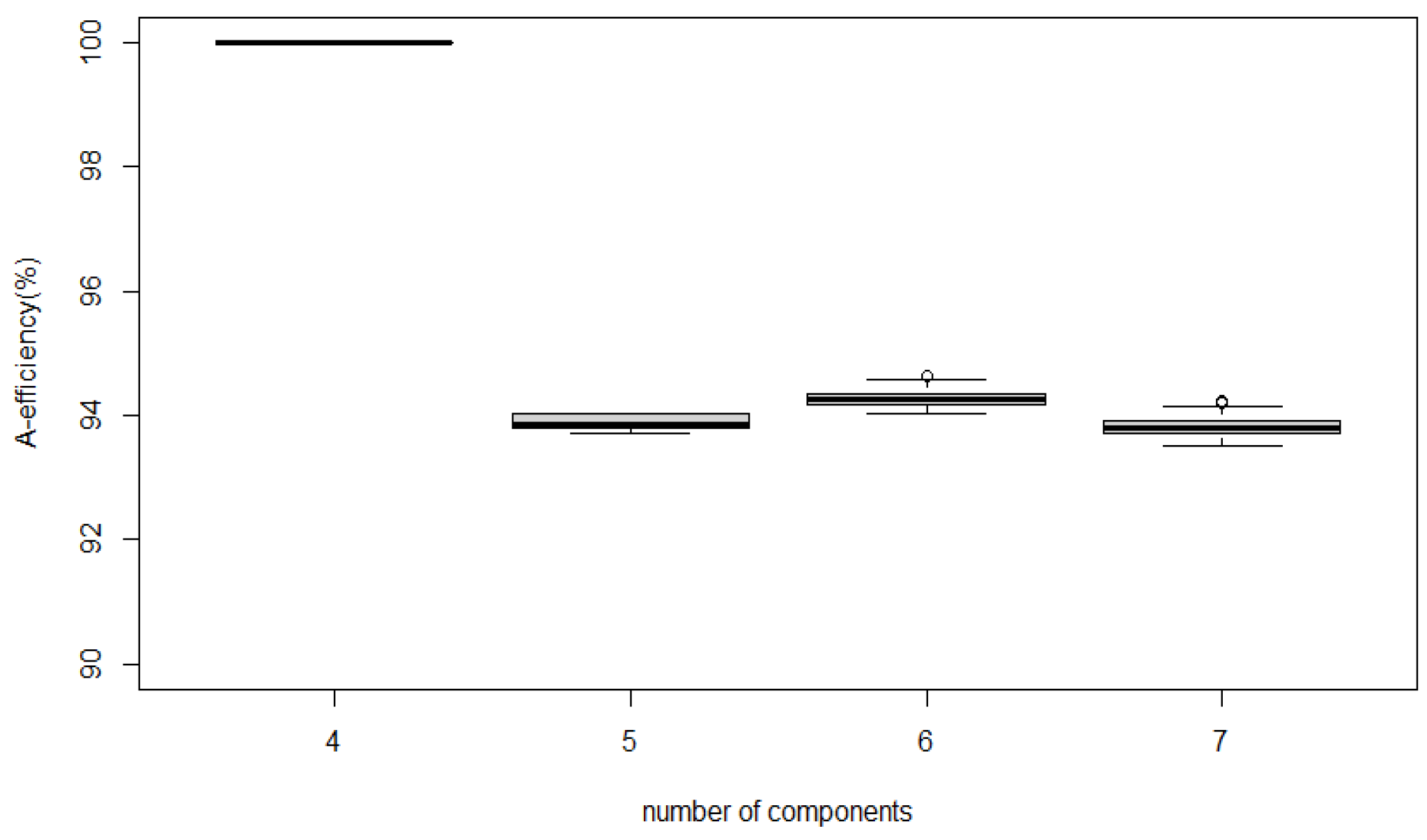
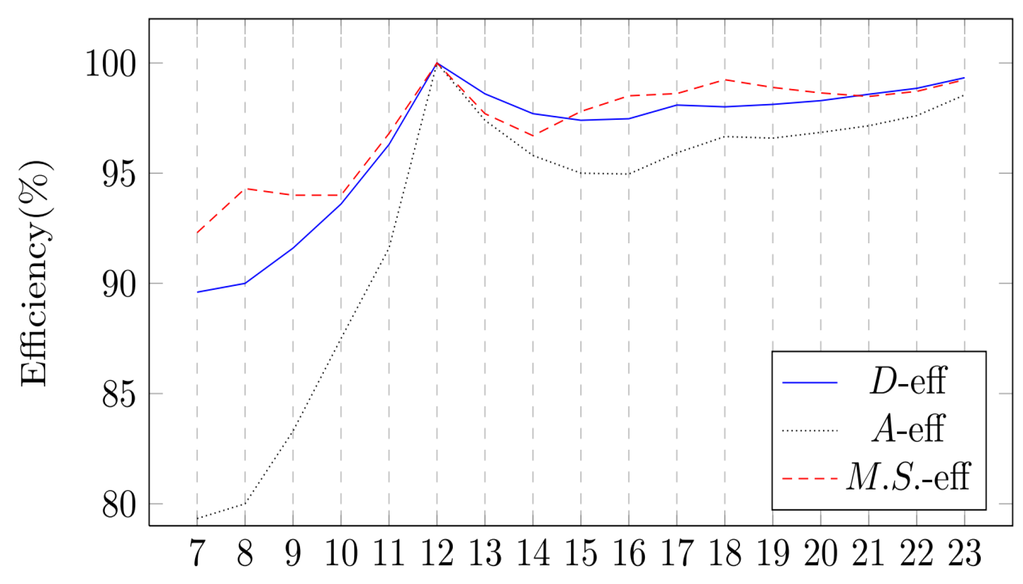
Furthermore, for the OofA experiment with four components, we generated optimal PWO designs with seven to 23 runs using the Ex-PSO algorithm. Figure 4 shows the efficiencies of these designs. All the obtained designs with $n\ge 12$ reach at least $95\%$ efficiency of the full PWO design, though with less than one-fifth of the runs. Especially for the cases with $n=12$, the design attains the same efficiency as the full PWO design.

Furthermore, we compare four types of fractional PWO designs, which are COA, and the corresponding designs obtained by the threshold-accepting algorithm [11], the Federov’s exchange algorithm (which iteratively optimizes a delta function of the $x_i$ and x where $x_i$ is in the design and x is not, see reference to Section 3.3 in [13],) and the Ex-PSO algorithm, denoted as $D_{coa}$, $D_{ta}$, $D_{ex}$ and $D_{ex-pso}$, respectively. $D_{ta}$ is the best result obtained over repeated runs of the threshold-accepting algorithm with up to $10,000,000$ iterations, $D_{ex}$ is generated by the optFederov function (implemented in the R library AlgDesign) with $nRepeats=5$, and $D_{ex-pso}$ is the best result obtained over five repeated runs of the Ex-PSO algorithm with $t_{ex}=20$ and $t_{pso}=100$. The optimal PWO design constructed by [4] which serves as a benchmark for evaluating fractional PWO designs is also listed here and denoted as $D_{peng}$. In addition, the new hybrid algorithm needs an exhaustive search over the design space during the single-point exchange procedure, and it can be computationally expensive if m is large. Hence, we only report designs with $n=m(m-1)/2+1,m(m-1),m!/r!(r=\lfloor m/2\rfloor )$ where $4\le m\le 7$. Nevertheless, given the tremendous growth in computational resources available, it is feasible to conduct the Ex-PSO algorithm for constructing designs with $m>7$.

Table 4, Table 5 and Table 6 exhibit the values of $det{(\tilde{M})}^{1/p}$, $tr({\tilde{M}}^{-1})$, $tr({\tilde{M}}^2)$, and D-, A- and $M.S.$-efficiency (in parentheses) for the corresponding designs. Note that the larger the value of $det{(\tilde{M})}^{1/p}$ is, the better, while smaller values of $tr({\tilde{M}}^{-1})$ and $tr({\tilde{M}}^2)$ are better. For any number of components, $D_{mp}$ is not unique and the corresponding $tr({\tilde{M}}^{-1})$ or $tr({\tilde{M}}^2)$ is by no means a fixed value. Hence, $D_{mp}$ is not listed in Table 5 and Table 6. From the tables, we can find that $D_{ex-pso}$ reaches a higher efficiency than the other types of designs under the PWO model in most cases. Further, we report the best PWO designs with $n=m(m-1)/2+1,m(m-1)$ and $4\le m\le 7$ under the D-, A- and $M.S.$-optimal criteria in

Table A1. D-Optimal PWO designs for $m=4$.

7 Runs				12 Runs
				Runs 1–7				Runs 8–12
1	2	3	4	1	2	4	3	3	2	1	4
1	3	4	2	1	2	3	4	3	2	4	1
2	1	4	3	1	3	4	2	4	1	3	2
3	1	2	4	2	1	4	3	4	2	1	3
3	2	4	1	2	3	4	1	4	2	3	1
4	1	3	2	3	1	4	2	4	3	1	2
4	2	3	1

,

Table A2. D-Optimal PWO designs for $m=5$.

11 Runs					20 Runs
					Runs 1–10					Runs 11–20
1	5	3	4	2	1	5	2	3	4	3	5	4	1	2
2	5	3	4	1	1	2	5	4	3	3	4	2	1	5
2	3	1	4	5	1	3	4	2	5	4	1	5	3	2
2	4	1	3	5	1	4	2	3	5	4	3	1	5	2
3	2	5	1	4	2	1	4	3	5	4	3	5	1	2
3	4	5	1	2	2	5	4	1	3	4	5	3	2	1
4	2	5	1	3	2	3	4	5	1	5	1	3	2	4
4	3	1	2	5	2	4	5	3	1	5	2	3	1	4
4	5	3	2	1	3	2	1	5	4	5	3	1	4	2
5	1	2	4	3	3	5	2	1	4	5	4	2	1	3
5	4	2	3	1

,

Table A3. D-Optimal PWO designs for $m=6$.

16 Runs						30 Runs
						Runs 1–15						Runs 16–30
1	6	5	2	4	3	1	6	2	5	3	4	4	5	1	6	2	3
1	2	4	5	3	6	1	2	6	3	5	4	4	5	2	6	1	3
1	5	3	6	4	2	1	3	4	2	5	6	4	5	3	1	2	6
2	1	3	5	4	6	1	4	6	3	5	2	5	2	1	3	6	4
2	3	6	5	4	1	2	1	5	4	6	3	5	2	3	1	4	6
3	1	4	2	6	5	2	6	4	1	5	3	5	4	1	3	6	2
3	2	5	1	6	4	2	3	5	4	6	1	5	4	3	6	1	2
3	4	5	1	6	2	3	1	5	2	6	4	5	6	3	1	2	4
4	1	3	5	2	6	3	1	6	4	2	5	5	6	3	4	2	1
4	2	5	1	6	3	3	2	6	5	1	4	6	1	5	4	2	3
4	3	6	5	2	1	3	2	4	1	6	5	6	1	2	3	4	5
5	2	6	3	1	4	3	4	6	1	5	2	6	2	1	4	5	3
5	4	6	3	1	2	3	5	6	2	1	4	6	2	4	3	5	1
6	1	4	2	3	5	4	2	1	3	5	6	6	3	5	4	2	1
6	3	2	4	1	5	4	2	6	5	3	1	6	5	1	3	2	4
6	5	1	3	2	4

,

Table A4. D-Optimal PWO designs for $m=7$.

22 Runs							42 Runs
							Runs 1–21							Runs 22–42
1	7	5	2	6	4	3	1	7	6	5	2	3	4	4	3	7	5	6	2	1
1	4	3	6	5	7	2	1	4	7	2	3	6	5	4	7	2	1	5	6	3
2	5	6	1	3	4	7	1	4	3	2	7	6	5	4	6	2	1	7	5	3
2	6	3	4	7	1	5	1	5	6	4	2	7	3	4	6	5	3	7	1	2
3	1	2	5	6	7	4	1	6	2	4	5	3	7	5	1	6	4	7	3	2
3	2	7	4	6	5	1	2	1	4	3	6	7	5	5	2	1	7	4	6	3
3	7	5	6	1	4	2	2	3	7	1	6	4	5	5	2	3	6	4	1	7
3	5	4	1	7	6	2	2	3	5	4	7	6	1	5	3	1	4	6	7	2
4	2	1	7	5	3	6	2	5	7	1	3	4	6	5	7	2	6	1	4	3
4	5	6	1	2	7	3	2	5	4	7	3	6	1	6	1	7	2	3	4	5
5	2	7	1	6	3	4	2	5	6	1	3	7	4	6	1	5	3	4	2	7
5	3	6	7	2	4	1	2	6	7	5	4	3	1	6	3	2	4	7	5	1
5	4	6	3	2	7	1	2	6	4	7	3	5	1	6	3	4	5	1	2	7
5	7	4	2	3	6	1	3	1	7	2	5	6	4	6	7	1	3	5	2	4
6	1	7	5	3	4	2	3	1	5	6	2	7	4	6	7	1	4	2	5	3
6	2	1	3	7	5	4	3	2	4	1	6	5	7	7	3	1	4	5	2	6
6	2	5	4	7	3	1	3	7	5	4	1	2	6	7	3	6	4	2	5	1
6	4	1	3	2	5	7	3	6	5	7	4	2	1	7	4	1	6	2	3	5
6	7	4	3	2	5	1	4	1	3	2	5	6	7	7	4	5	3	6	1	2
7	1	3	2	5	4	6	4	1	5	7	3	2	6	7	6	3	2	1	5	4
7	1	4	6	2	5	3	4	2	6	3	1	5	7	7	6	5	4	1	3	2
7	6	3	2	1	4	5

,

Table A5. A-Optimal PWO designs for $m=4$.

7 Runs				12 Runs
				Runs 1–7				Runs 8–12
1	3	4	2	1	4	3	2	3	1	2	4
2	1	4	3	1	2	3	4	3	2	4	1
2	3	1	4	2	1	3	4	3	4	2	1
3	1	2	4	2	1	4	3	4	1	3	2
3	2	4	1	2	4	3	1	4	1	2	3
4	1	2	3	3	1	4	2	4	2	3	1
4	3	2	1

,

Table A6. A-Optimal PWO designs for $m=5$.

11 Runs					20 Runs
					Runs 1–10					Runs 11–20
1	4	2	3	5	1	5	3	4	2	3	5	1	4	2
2	1	5	4	3	1	2	5	4	3	3	5	2	4	1
2	1	3	4	5	1	3	2	4	5	4	1	5	2	3
2	3	5	4	1	2	1	4	3	5	4	2	1	3	5
2	4	5	1	3	2	5	4	3	1	4	2	5	1	3
3	4	1	2	5	2	3	5	4	1	4	3	1	5	2
4	1	3	5	2	2	3	4	1	5	4	5	3	2	1
4	3	2	5	1	3	1	4	2	5	5	1	2	4	3
4	5	2	3	1	3	2	1	5	4	5	2	3	1	4
5	1	3	4	2	3	2	4	5	1	5	4	1	3	2
5	3	1	2	4

,

Table A7. A-Optimal PWO designs for $m=6$.

16 Runs						30 Runs
						Runs 1–15						Runs 16–30
2	1	5	6	3	4	1	3	2	6	4	5	4	1	5	2	3	6
3	1	2	4	5	6	1	3	5	6	2	4	4	2	1	3	5	6
3	1	6	4	5	2	1	4	2	6	3	5	4	3	2	5	6	1
3	5	2	4	1	6	1	4	3	6	2	5	4	6	1	2	3	5
3	5	6	4	1	2	2	1	6	4	5	3	4	5	1	6	3	2
4	2	3	6	5	1	2	1	6	3	5	4	5	2	3	1	4	6
4	3	6	2	1	5	2	1	4	5	6	3	5	2	4	6	1	3
4	5	6	2	3	1	2	3	5	1	6	4	5	3	4	1	2	6
5	1	6	4	3	2	2	5	3	6	4	1	5	6	1	3	4	2
5	1	3	4	6	2	2	5	4	3	1	6	6	1	4	2	5	3
5	3	2	6	1	4	3	1	2	5	4	6	6	2	1	5	3	4
6	1	5	2	4	3	3	1	4	5	6	2	6	2	3	4	5	1
6	1	3	4	5	2	3	2	4	6	1	5	6	4	3	1	5	2
6	2	3	5	1	4	3	4	6	5	2	1	6	5	1	2	4	3
6	2	4	5	1	3	3	5	2	6	1	4	6	5	4	3	2	1
6	5	3	4	1	2

,

Table A8. A-Optimal PWO designs for $m=7$.

22 Runs							42 Runs
							Runs 1–21							Runs 22–42
1	3	7	4	2	6	5	1	2	7	3	5	4	6	4	7	3	6	1	5	2
1	5	4	6	3	7	2	1	3	7	6	5	2	4	4	7	6	1	2	5	3
1	6	7	4	5	3	2	1	5	4	6	3	7	2	4	5	2	1	3	6	7
1	6	3	4	5	7	2	1	6	2	5	3	4	7	5	1	7	4	3	6	2
2	7	6	1	4	3	5	1	6	4	7	3	2	5	5	3	6	4	1	7	2
2	4	5	6	1	3	7	1	6	4	5	2	7	3	5	7	3	2	4	1	6
2	6	5	4	3	1	7	2	1	4	5	7	6	3	5	7	3	6	1	4	2
3	6	1	5	7	2	4	2	7	6	5	1	4	3	5	6	4	3	1	2	7
3	6	2	5	1	4	7	2	4	3	5	6	7	1	6	1	7	3	5	2	4
3	6	4	2	7	1	5	2	4	5	6	1	3	7	6	1	3	4	5	2	7
4	1	6	2	7	3	5	2	6	5	4	7	1	3	6	1	5	3	7	4	2
4	1	5	2	7	3	6	3	1	2	4	6	7	5	6	2	3	5	1	4	7
4	2	3	5	6	7	1	3	1	7	2	6	4	5	6	2	4	1	7	5	3
4	3	1	7	5	6	2	3	2	7	1	5	4	6	6	3	5	2	7	4	1
4	7	6	5	3	1	2	3	4	2	1	7	5	6	6	7	4	3	1	2	5
5	3	2	7	4	1	6	3	4	5	7	1	2	6	6	7	5	2	3	1	4
5	6	3	1	4	2	7	3	6	2	7	1	4	5	7	1	5	2	6	4	3
7	1	6	2	4	5	3	4	2	6	3	1	5	7	7	2	1	3	5	6	4
7	1	3	2	5	6	4	4	2	6	7	5	1	3	7	4	5	1	6	2	3
7	5	2	3	1	4	6	4	2	3	1	6	5	7	7	5	2	6	3	1	4
7	6	3	4	2	1	5	4	3	7	6	5	2	1	7	6	3	4	2	5	1
7	6	5	4	2	1	3

,

Table A9. $M.S.$-Optimal PWO designs for $m=4$.

7 Runs				12 Runs
				Runs 1–7				Runs 8–12
1	2	4	3	1	4	3	2	2	3	1	4
2	1	3	4	1	4	2	3	3	2	1	4
2	4	3	1	1	2	3	4	3	4	1	2
3	1	4	2	1	3	2	4	3	4	2	1
3	2	4	1	2	4	1	3	4	2	1	3
4	1	3	2	2	4	3	1	4	3	1	2
4	2	1	3

,

Table A10. $M.S.$-Optimal PWO designs for $m=5$.

11 Runs					20 Runs
					Runs 1–10					Runs 11–20
1	5	2	4	3	1	5	3	4	2	3	5	2	1	4
1	5	3	4	2	1	2	5	4	3	4	1	3	2	5
1	3	2	4	5	1	3	4	5	2	4	2	5	1	3
2	5	1	4	3	2	1	4	3	5	4	2	3	1	5
2	5	3	4	1	2	1	5	3	4	4	3	1	5	2
2	3	1	4	5	2	3	1	4	5	4	5	1	2	3
3	5	1	4	2	2	3	4	5	1	4	5	3	2	1
3	5	2	4	1	3	1	4	2	5	5	1	2	4	3
4	1	2	3	5	3	2	5	4	1	5	3	2	4	1
4	3	2	1	5	3	5	1	4	2	5	4	2	3	1
4	5	2	1	3

,

Table A11. $M.S.$-Optimal PWO designs for $m=6$.

16 Runs						30 Runs
						Runs 1–15						Runs 16–30
1	2	6	4	5	3	1	4	2	3	5	6	4	2	1	6	3	5
1	3	4	6	5	2	1	4	3	2	6	5	4	5	6	2	3	1
1	5	2	4	3	6	1	4	5	3	6	2	5	1	6	3	4	2
2	6	3	4	5	1	2	1	6	5	3	4	5	1	2	6	4	3
2	5	1	3	4	6	2	6	4	5	1	3	5	2	1	3	4	6
3	2	6	1	5	4	2	3	5	6	1	4	5	3	1	2	4	6
3	4	1	2	5	6	2	3	4	1	5	6	5	3	6	4	2	1
3	5	1	6	4	2	2	4	6	5	3	1	5	4	2	3	6	1
4	1	3	6	2	5	3	1	6	5	2	4	5	4	6	1	3	2
4	2	3	5	6	1	3	2	5	4	1	6	6	1	2	3	4	5
4	6	5	3	1	2	3	2	6	4	1	5	6	2	1	5	4	3
5	3	6	2	4	1	3	4	6	2	5	1	6	3	1	4	2	5
5	4	2	1	6	3	3	4	6	5	1	2	6	3	1	5	2	4
5	6	1	4	3	2	4	1	3	5	2	6	6	4	3	5	2	1
6	1	2	3	5	4	4	1	6	2	5	3	6	5	4	1	2	3
6	4	2	1	5	3

,

Table A12. $M.S.$-Optimal PWO designs for $m=7$.

22 Runs							42 Runs
							Runs 1–21							Runs 22–42
1	2	3	6	7	4	5	1	7	2	6	3	4	5	4	2	6	7	3	5	1
1	2	5	7	6	3	4	1	7	2	4	5	6	3	4	3	5	1	7	2	6
1	4	3	6	2	5	7	1	7	5	3	2	6	4	4	7	5	3	2	1	6
2	1	6	5	4	3	7	1	3	2	5	7	4	6	4	5	3	6	2	1	7
2	5	4	6	3	1	7	1	3	4	5	6	2	7	4	5	7	6	2	1	3
3	4	1	7	5	6	2	1	4	3	2	6	7	5	4	6	3	7	1	5	2
3	4	2	7	6	5	1	1	5	7	4	2	3	6	5	2	1	6	4	3	7
4	5	2	6	7	1	3	1	6	5	2	4	7	3	5	3	2	4	7	6	1
4	5	3	1	7	2	6	2	7	5	1	3	4	6	5	4	1	6	3	7	2
4	6	1	7	2	5	3	2	3	4	1	6	5	7	5	7	4	2	3	6	1
5	2	1	7	3	4	6	2	3	5	6	4	7	1	5	6	7	3	1	2	4
5	3	6	1	7	4	2	2	4	7	6	1	5	3	6	1	4	2	5	3	7
5	3	6	2	4	7	1	2	4	3	7	1	6	5	6	1	5	3	4	7	2
6	1	4	5	7	3	2	2	5	3	7	1	4	6	6	2	5	1	7	4	3
6	3	2	1	7	4	5	2	6	3	1	7	5	4	6	5	3	4	1	2	7
6	3	5	7	1	2	4	3	1	4	6	7	2	5	6	7	2	5	4	1	3
6	7	5	4	2	3	1	3	2	6	4	5	1	7	6	7	4	5	1	2	3
7	1	5	4	6	3	2	3	7	6	4	2	5	1	7	1	3	6	5	4	2
7	2	4	3	1	5	6	3	7	5	6	1	2	4	7	4	6	1	3	2	5
7	3	2	6	1	5	4	3	6	7	2	1	4	5	7	5	3	4	1	2	6
7	5	1	3	2	4	6	4	2	1	7	5	6	3	7	6	3	5	2	1	4
7	6	2	4	5	1	3

in appendix.

We conclude this section with some numerical results on constructions of fractional PWO designs which have the same correlation structure as the full PWO design. Since these designs are 100% efficient under diverse design criteria including the D-, A-, $M.S.$-optimal criteria, we call them fully efficient PWO designs. Using the Ex-PSO algorithm, we find the following results.

Remark 3. 

Removing $p (<m)$ components from a fully efficient PWO design with m components will result in a fully efficient PWO design with $m-p$ components.

Remark 4. 

The fully efficient PWO designs exist for the cases (i) $m=4,5$, $n=12k (k\ge 1)$; (ii) $m=6$, $n=24k (k\ge 1)$; and (iii) $m=7$, $n=24.$

For saving space, some selected fully efficient PWO designs with minimized runs for $m=4,5,6,7$ are exhibited in

Table 7. Selected fully efficient PWO designs for $m=4,5,6,7$.

$\mathit{m}=4$	$\mathit{m}=5$	$\mathit{m}=6$		$\mathit{m}=7$
		Runs 1–12	Runs 13–24	Runs 1–12	Runs 13–24
1 2 4 3	1 2 3 5 4	1 2 5 4 6 3	4 2 1 3 6 5	1 2 3 7 4 6 5	4 5 2 6 7 1 3
1 3 4 2	1 4 3 5 2	1 2 5 4 6 3	4 2 5 3 6 1	1 5 6 3 2 7 4	4 6 3 7 1 2 5
1 3 2 4	1 5 3 2 4	1 3 4 2 5 6	4 6 3 2 5 1	1 6 5 7 4 2 3	4 7 1 3 6 5 2
2 1 4 3	2 4 3 1 5	1 3 6 2 5 4	5 1 2 4 3 6	1 7 4 3 2 5 6	5 2 4 3 6 1 7
2 3 1 4	2 5 1 4 3	1 4 6 5 2 3	5 4 3 2 1 6	2 5 4 1 7 6 3	6 1 2 4 5 7 3
2 3 4 1	3 1 4 2 5	2 3 4 5 1 6	5 2 1 6 3 4	2 7 6 3 1 5 4	6 4 2 1 3 7 5
3 1 4 2	3 2 4 5 1	2 6 1 5 3 4	5 3 6 2 1 4	3 2 1 6 4 7 5	6 5 1 3 4 7 2
3 2 4 1	3 5 4 2 1	2 6 4 3 1 5	5 6 4 1 2 3	3 2 6 5 7 4 1	6 7 2 3 4 5 1
4 1 2 3	4 2 1 5 3	3 1 2 6 4 5	6 2 1 4 3 5	3 4 1 5 7 2 6	7 4 6 5 3 2 1
4 2 1 3	4 5 1 2 3	3 1 5 6 4 2	6 2 5 3 4 1	3 5 1 4 6 2 7	7 2 1 5 3 4 6
4 3 1 2	5 2 3 1 4	3 5 2 4 6 1	6 3 5 1 4 2	3 5 7 6 2 1 4	7 5 1 2 6 4 3
4 3 2 1	5 4 3 1 2	4 1 5 6 3 2	6 4 5 1 3 2	4 2 5 3 7 1 6	7 5 3 6 4 1 2

, other fully efficient PWO designs and the MATLAB codes for the Ex-PSO algorithm are available upon request.

6. Concluding Remarks

In this article, we have presented a new hybrid algorithm for searching optimal PWO designs for OofA experiments. This algorithm starts with a set of randomly selected particle designs. It combines the single-point exchange algorithm for generating the local-best design related to each particle and the PSO algorithm for clustering the particle designs gradually around the global optimal design. We have addressed two points for this stochastic optimization technique: (i) the selection of initial particle designs; and (ii) the definition of the particle designs’ movement toward its personal local-best or global-best design. As the sample space is a large combinatorial set of $m!$ points, it’s satisfying to randomly select points for initial designs. In addition, the movement is defined as randomly exchanging points to adjust the particle design toward the target design. Our generated design has an appealing efficiency in comparison with the full PWO design, though with only a small fraction of runs. It also achieves better efficiency compared with the existing designs. In addition, we have reported optimal PWO designs and some selected 100% efficient PWO designs for application.

To illustrate the effectiveness of our model and designs, we provide a real-life OofA experiment. The data is from the four-drug data in Table 3 of [8]. The first-order PWO model fits using the data from the fully efficient PWO design with 12 runs (runs {1,2,6,7,10,11,16,18,20,21,22,24} of four-drug data) as well as the full design with 24 runs (i) with an adjusted R square of 0.93 (vs. 0.77), (ii) an RMSE of 2.19 (vs. 3.53) based on 5 (vs. 17) degrees of freedom. For further comparison, we consider variable selection to simplify the first-order PWO model. We start with a model with intercept only and perform stepwise regression with the AIC criterion. By using the data of fully efficient design, the stepwise regression leads to the following PWO model: $y=44.22-3.82z_{23}+6.02z_{34}+2.79z_{12}-2.96z_{14}+1.37z_{13}$, which has an adjusted R square of 0.95, an RMSE of 2.00 with 6 degrees of freedom. When using the data of full design, the stepwise regression leads to the following PWO model: $y=45.22-3.91z_{12}+3.86z_{23}-1.59z_{13}$, which has an adjusted R square of 0.79, an RMSE of 3.43 with 20 degrees of freedom. Thus, the first-order PWO model is sufficient for the four-drug OofA experiment. Meanwhile, the fully efficient design has an appealing efficiency, though with only a half run of the full design. However, in some applications, we are persuaded that the first-order PWO model cannot account for all systematic effects caused by component ordering; thus, we shall consider the second-order PWO model to obtain a lower error. This approach can be referred to [7].

In addition, from the viewpoint of model robustness, it is interesting to examine how our designs behave under high-order PWO models. From the perspective of model parsimony, we only consider the second-order PWO model with only a few interactions of two PWO factors sharing a common component being entertained, and recommend using the fully efficient PWO designs for analysis. We omit the details to save space but note that, even under such augmented models, the fully efficient PWO designs tend to perform well, particularly under the D-, $M.S.$-criteria and often under the A-criterion. For example, the fully efficient design for $m=6,n=24$, has D-, A-, $M.S.$-efficiencies of at least 90%, under such augmented model. This allows further flexibility in model selection with a provision for penalty for the additional parameters that correspond to two-factor interactions. As before, one remains assured of relatively high design efficiency under the model that one arrives at.

As pointed out by reviewers, our work can be extended using alternation optimization techniques, such as the memetic optimization algorithm based on local searches [19]. We conclude with the hope that the present endeavor will generate further interest in optimal designs for OofA experiments and related topics.