Improving Stock Market Predictions: An Equity Forecasting Scanner Using Long Short-Term Memory Method with Dynamic Indicators for Malaysia Stock Market

Abstract

Stock market predictions are a challenging problem due to the dynamic and complex nature of financial data. This study proposes an approach that integrates the domain knowledge of investors with a long-short-term memory (LSTM) algorithm for predicting stock prices. The proposed approach involves collecting data from investors in the form of technical indicators and using them as input for the LSTM model. The model is then trained and tested using a dataset of 100 stocks. The accuracy of the model is evaluated using various metrics, including the average prediction accuracy, average cumulative return, Sharpe ratio, and maximum drawdown. The results are compared to the performance of other strategies, including the random selection of technical indicators. The simulation results demonstrate that the proposed model outperforms the other strategies in terms of accuracy and performance in a 100-stock investment simulation, highlighting the potential of integrating investor domain knowledge with machine learning algorithms for stock price prediction.

1. Introduction

Stock forecasting is a critical task for investors, financial analysts, and computer scientists. Accurate stock price predictions can help investors make informed trading decisions, resulting in significant benefits. However, stock price prediction is a complex problem due to the numerous variables that can affect stock prices, such as economic conditions, market trends, company news, and geopolitical events. Therefore, developing a reliable and accurate model for stock price prediction is a challenging task.

Traditional methods of stock price prediction, such as technical analysis, involve analyzing historical stock data manually to identify trading opportunities [1]. However, analyzing large amounts of data manually can be time-consuming and challenging for investors. To overcome these limitations, researchers have turned to machine learning techniques to help predict stock prices. Machine learning algorithms can handle vast amounts of complex data, identify hidden patterns, and reveal complex relationships that are difficult to detect manually.

Recent research has shown that combining machine learning algorithms with technical and fundamental indicators can improve stock price prediction efficiency by 60% to 80% [2]. However, most previous works lack flexibility and dynamism in their prediction models. Previous works have employed feature selection algorithms to filter out the most popular features, but this approach can result in input that is full of randomness and excludes essential technical indicators specific to a stock. Therefore, a better solution is to allow domain users, such as investors, to customize the prediction model using their preferred indicators as input parameters.

This paper aims to fill the gap in the stock price prediction model’s lack of flexibility and dynamism, enabling investors to make more meaningful predictions that will assist them in making informed trading decisions. In this paper, we propose a novel approach to stock forecasting using LSTM with dynamic indicators that incorporates investor domain knowledge and outperforms the traditional approach of randomly selecting technical indicators as input. We have conducted an extensive evaluation of the proposed model using a dataset of 100 stocks from the Malaysian stock market, demonstrating superior prediction accuracy, cumulative return, and risk performance compared to existing approaches. We provide evidence that integrating the domain knowledge of investors into the prediction model can significantly enhance the accuracy and performance of the model. We demonstrate the effectiveness of LSTM models in capturing the temporal dependencies and patterns in stock market data, enabling accurate and reliable forecasting.

The remaining sections of this paper are organized as follows: Section 2 will cover related work on machine learning algorithms used for equity forecasting; Section 3 will cover the design of the proposed model using the LSTM method; Section 4 will cover the experiments to evaluate the effectiveness of the proposed model; Section 5 will cover the results of the experiments for four different strategies: article model, buy-and-hold, optimistic model, and the proposed model; Section 6 will cover the discussion on the outcome of the proposed model; and Section 7 will cover the conclusion of this paper.

2. Related Works

In recent times, stock prices have become increasingly dynamic and volatile due to the easy availability of information through technology such as social media and online news. This has led to a greater number of reactions to stocks, resulting in high volatility in stock prices in the market. Predicting stock prices, therefore, heavily relies on the analysis of vast amounts of data, which is where machine learning comes into play. Machine learning algorithms such as evolutionary algorithms (e.g., genetic algorithms (GAs) [3]), artificial neural networks (ANNs), long-short-term memory (LSTM), and support vector machines (SVMs) are widely used as stock price prediction models [4,5].

In today’s dynamic and volatile stock markets, machine learning algorithms play a crucial role in predicting stock prices. Genetic algorithms (GAs), which are a type of evolutionary algorithm, are one such algorithm that has been widely used to optimize the combination of technical indicators for maximum trading profits.

A recent study [6] proposed a stock trading model based on optimized technical indicators using GAs. The authors used historical stock prices of Dow Jones’, New York, NY, USA, 30 stocks from 1997 to 2017 as training data to determine the best parameters for relative strength index (RSI) and simple moving average (SMA) combinations in the time series of the stocks. They then used these optimized technical indicators as input features in a deep neural network (DNN) to predict the buy and sell positions. The results showed that the GA+DNN model achieved 11.93% of the average annualized return of 30 stocks, which was better than the model that used random technical indicators. The GA was able to determine the important technical indicators that had yielded the highest results in the past and solved the difficulty of setting the hyperparameters for different stock indicators.

However, one limitation of this approach is that the selection of GA hyperparameters such as crossover rate and mutation rate should be determined carefully to avoid meaningless combinations of technical indicators. Furthermore, when a GA is used in the feature optimization process, more hyperparameters (GAs hyperparameters and neural networks’ hyperparameters) need to be fine-tuned during the training process, which requires more time.

Another study [7] used GAs to optimize the hyperparameters of different technical indicators for trading rules. They considered a total of six technical indicators with different meanings and adopted GAs to find a trading rule that had generated the highest profit in the past. The results showed that the derived strategies generated an average profit of 21% to 54% even though the index of the India Cement Stock Price Index (ICSPI), New Delhi, India, was decreasing during the validation period. However, this approach does not account for the movement behavior of stocks throughout history, which is important for investors’ decision-making. Therefore, it is better to include the optimized trading rules as input parameters for machine learning models to learn the movement behavior of stocks.

In conclusion, GAs have shown consistent results in finding the best hyperparameters of technical indicators for generating positive profits in the stock market. However, some limitations need to be addressed, such as the careful selection of hyperparameters and the consideration of stock movement behavior in the decision-making process.

In addition to GAs, artificial neural networks (ANNs) are also often used to predict stock prices. According to [8], the ANN model is the most commonly used machine learning model in stock price prediction. An ANN is designed to simulate the processing of information by human brain cells, which enables it to learn complex, nonlinear relationships between data. One limitation of an ANN is that it cannot detect the long-term dependency between historical prices.

In [9], the authors used ANNs to forecast the S&P 500 index, New York, USA, based on 60 financial and fundamental features (2003–2013 period). They used fuzzy c-means clustering (FCM) and principal component analysis (PCA) to reduce the complexity of the input data and extract the features that had a strong relationship with the stock index. PCA is a powerful unsupervised linear technique for feature extraction and dimension reduction, and FCM is a well-known data clustering technique. The pre-processed data was then supplied to ANNs to make predictions. The results showed that the introduction of PCA techniques not only reduced the complexity of the data but also increased the prediction accuracy of the ANN model. The maximum accuracy achieved was about 59%. The ANN model was also evaluated in a trading simulation to find out whether the high predictability of ANN models implies high returns in stock trading. The trading simulation results proved that incorporating PCA with ANNs generated higher returns than the benchmark technical analysis buy-and-sell strategy.

In [10], the authors used the National Association of Securities Dealers Automated Quotations (NASDAQ), New York, NY, USA, stock market index for 2017 and 2018 as training data. They considered both technical indicators and financial news as extra features in prediction, resulting in 151 to 611 dimensions in the input dataset. They used the synthetic minority over-sampling technique (SMOTE) to balance the label and the increasing window cross-validation method to preserve the time series behavior of the data during the validation process. They also introduced dropout layers in the ANN model to avoid overfitting issues. The results showed that the ANN model achieved between 50% and 68% accuracy on average, an 85.2% positive annualized return, and a 4.6% Sharpe ratio in the trading simulation. The strength of the approach proposed by this study is that the model not only considers technical, fundamental, and sentiment data from financial news but also focuses on retaining the time series behavior of stock prices during the validation process.

Overall, all the above ANN models have shown consistent results in both machine learning validation and trading simulation. To increase the overall performance of the stock prediction model, [9] applied feature engineering techniques such as FCM and PCA, while [10] balanced the label and retained the time series behavior of the data during the validation process. However, they have limitations, such as the inability of ANNs to detect long-term dependence between historical prices and the loss of information after applying PCA components to the technical indicators. To address these limitations, the LSTM algorithm can be used, as it can capture both non-linearity and sequential information in the data.

The LSTM is a powerful time series model that is derived from the recurrent neural network (RNN) structure [11,12]. Unlike RNNs, LSTM can memorize long-term sequential information by using extra memory lines and control gates, making it a suitable algorithm for time series problems such as stock prediction [13]. In the traditional RNN structure, the neural network concatenates the hidden layer output of the previous time step (h_t−1) with the input of the next time step (x_t), and these procedures are repeated until the latest time frame of input data is reached. However, the RNN structure has a limitation in that it is not able to store long-term memory and tends to put more emphasis on recent memory, resulting in difficulty in capturing long-term dependencies in the data. LSTM solves this problem by having extra gates that control the information stored in memory, allowing it to decide which past information is valuable in making predictions and thus memorizing long-term dependencies in the data. Figure 1 illustrates the working procedure of a single unit of LSTM.

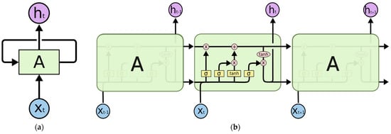
Figure 1. Single unit of an LSTM cell (folded and unfolded) [14]: (a) recurrent neural networks have loops; (b) the repeating module in an LSTM contains four interacting layers.

Each time-step X_t−1, X_t, and X_t+1 will go through the LSTM unit that is named “A”. Each time step will result in hidden state outputs h_t−1, h_t, and h_t+1, respectively, and all-time steps will go through the same unit. The hidden state output produced at each time step would also be brought to another time step so that the time dependency could be learned by the model. LSTM is suitable for any problem that involves sequential information, such as stock forecasting, traffic prediction [15], etc.

Two papers have been reviewed that compare the performance of LSTM and ANNs in the stock forecasting domain. [16] conducted research on combining optimal technical indicators with LSTM in stock prediction and compared the performance of LSTM with that of ANN and SVM models. The results show that using optimal technical indicators produces promising results, with the highest accuracy of 64% achieved by LSTM. In comparison with other models, LSTM outperformed other models when supplied with relevant input parameters, reducing its complexity, and increasing its performance. [17] conducted comprehensive research that compared the performance of LSTM, ANNs, and uncertainty-aware attention (UA) in stock price prediction using different types of market environments. The results showed that LSTM and UA models performed better than ANNs in developing and less developed markets, where time series algorithms are more suitable for handling such data.

In both papers, evaluating the algorithm in the stock forecasting problem is divided into two methods: machine learning evaluation and trading simulation evaluation. Prediction accuracy is calculated in machine learning evaluation, while in trading simulation evaluation, the model is evaluated as a trading system, and popular portfolio metrics such as percentage return and risk metrics (Sharpe ratio, Sortino ratio, and maximum drawdown) are calculated to measure the overall trading portfolio performance.

In conclusion, the previous literature has shown that technical indicators alone are insufficient for accurate stock trend prediction, with state-of-the-art performance typically ranging from 50% to 70% [18,19,20,21]. As such, it is essential to explore other data sources to improve the accuracy of stock forecasting. In our proposed method, we aim to integrate the domain knowledge of investors with an LSTM algorithm to improve its overall performance for predicting stock prices.

3. Methods

Figure 2 shows the process of obtaining the optimal LSTM model for the proposed model.

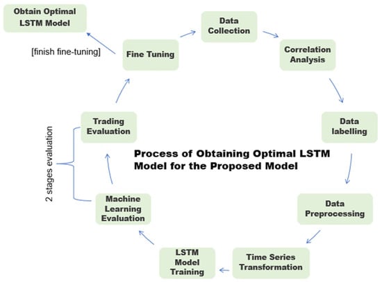
Figure 2. Process of obtaining the optimal LSTM model for the proposed model.

The design of the proposed model involved nine stages (see Figure 2) to determine the optimal LSTM model. Many possible technical indicator combinations will be used to study and obtain the optimal LSTM model so that the proposed model can closely simulate the real-world situation where many investors will use different indicator combinations as the input to the real-time model. Thus, the goal is to determine the optimal LSTM model that can accommodate and achieve averagely promising results across all 100 stocks with different types of input indicator combinations. Each stage of the process of obtaining the optimal LSTM model for the proposed model is discussed as follows:

3.1. Data Collection

The development of a prediction model starts with collecting stock data from historical prices of the selected stock using the Yahoo Finance API provided by the Python (Python Software Foundation, Fredericksburg, Virginia) platform. This data includes the open, close, high, low, volume, and adjusted closing prices of 100 selected stocks listed on Bursa Malaysia, Kuala Lumpur, Malaysia, (see Table 1) from the beginning of the listing to 30 June 2022.

Table 1. A list of the 100 selected stocks listed on Bursa Malaysia.

Stock Listing Code in Bursa Malaysia (.KL)
6888.KL	5225.KL	6033.KL	5139.KL	5210.KL	5398.KL	7153.KL	5236.KL	5279.KL	4588.KL
1023.KL	1961.KL	4065.KL	5099.KL	1818.KL	0078.KL	5878.KL	3069.KL	5288.KL	5005.KL
7277.KL	2445.KL	8869.KL	2488.KL	2852.KL	2291.KL	6633.KL	5286.KL	7155.KL	5292.KL
6947.KL	1155.KL	1295.KL	1015.KL	2836.KL	0208.KL	5284.KL	9385.KL	8664.KL	6963.KL
3182.KL	6012.KL	1066.KL	6399.KL	7204.KL	5102.KL	3859.KL	0138.KL	5211.KL	0097.KL
4715.KL	3816.KL	4197.KL	8176.KL	1619.KL	3255.KL	5264.KL	5258.KL	5176.KL	5246.KL
3034.KL	5296.KL	5285.KL	5106.KL	7148.KL	3301.KL	5014.KL	7160.KL	7106.KL	7293.KL
5168.KL	4707.KL	4863.KL	1562.KL	5222.KL	5227.KL	1171.KL	7084.KL	6139.KL	4677.KL
5819.KL	5183.KL	5347.KL	5248.KL	3689.KL	3336.KL	3867.KL	5218.KL	5031.KL	5109.KL
1082.KL	5681.KL	7113.KL	4162.KL	0128.KL	0166.KL	1651.KL	4731.KL	5148.KL	6742.KL

In addition, the data between 1 January 2019 and 30 June 2022 will be used for the simulation, while the remaining data (before 1 January 2019) will be used as a model training dataset. A feature expansion will then be carried out based on this data. One crucial aspect of feature expansion is calculating 22 technical indicators: exponential moving average, simple moving average, sum over period, minimum in period, maximum in period, Aroon, Adx, moving average convergence divergence, momentum, commodity channel index, relative strength index, Williams %R, price rate-of-change, stochastic relative strength index, volatility ratio, standard deviation, variance, standard error, on-balance volume, Bollinger bands, volume oscillator, and linear regression, which can be customized by the investor based on their preferences (see Table 2).

Table 2. A list of indicators used for the proposed model.

Indicators	Formula
Exponential Moving Average	$f\left(c,N\right)={price}_c\ast \frac{2}{(N+1)}+f\left(c-1,N\right)\ast (1-\frac{2}{(N+1)})$
Simple Moving Average	$f\left(N\right)=\frac{1}{N}{\displaystyle \sum _{i=1}^N}{price}_i$
Sum Over Period	$f\left(c,N\right)={\displaystyle \sum _{i=0}^{N-1}}{price}_{c-i}$
Minimum In Period	$f\left(c,N\right)=\mathrm{m}\mathrm{i}\mathrm{n}[{price}_c,{price}_{c-1},\cdots ,{price}_{c-N+1}]$
Maximum In Period	$f\left(c,N\right)=\mathrm{m}\mathrm{a}\mathrm{x}[{price}_c,{price}_{c-1},\cdots ,{price}_{c-N+1}]$
Aroon	$f_{up}\left(c,N\right)=\frac{N-\mathrm{m}\mathrm{a}\mathrm{x}[{price}_c,{price}_{c-1},\cdots ,{price}_{c-N+1}]}{N}\ast 100$ $f_{down}\left(c,N\right)=\frac{N-\mathrm{m}\mathrm{i}\mathrm{n}[{price}_c,{price}_{c-1},\cdots ,{price}_{c-N+1}]}{N}\ast 100$
Average Directional Index	$h_{+DI}(c,N)=\left(\frac{{\sum }_{i=c}^{N-1}{(high}_i-{high}_{i-1})-\left(\frac{{\sum }_{i=c}^{N-1}{(high}_i-{high}_{i-1})}{N}\right)+{(high}_c-{high}_{c-1})}{average true range}\right)\ast 100$ $h_{-DI}\left(c,N\right)=\left(\frac{{\sum }_{i=c}^{N-1}{(low}_{i-1}-{low}_i)-\left(\frac{{\sum }_{i=c}^{N-1}{(low}_{i-1}-{low}_i)}{N}\right)+{(low}_{c-1}-{low}_c)}{average true range}\right)\ast 100$ $g(c,N)=\left(\frac{\left|h_{+DI}(c,N)-h_{-DI}(c,N)\right|}{\left|h_{+DI}(c,N)+h_{-DI}(c,N)\right|}\right)$ $f\left(c,N\right)=\frac{\left(avg[g\left(c-1\right),\cdots ,g(c-N\left)\right]\ast (N-1)\right)+g\left(c\right)}{N}$
Moving Average Convergence Divergence	$f\left(c,N_1,N_2\right)=g\left(c,N_1\right)-g(c,N_2)$ $g\left(c,N\right)={price}_t\ast \frac{2}{(N+1)}+f\left(c-1,N\right)\ast (1-\frac{2}{(N+1)})$
Momentum	$f\left(c,m\right)={close}_c-{close}_{c-m}$
Commodity Channel Index	$f\left(N\right)=\frac{g\left(N\right)-h\left(N\right)}{0.015\ast \left(\frac{{\sum }_{i=1}^n\left|g\left(N\right)-h\left(N\right)\right|}{nN}\right)}$ $g\left(N\right)={\displaystyle \sum _{i=1}^N}\left(\frac{{high}_i+{low}_i+{close}_i}{3}\right)$ $h\left(N\right)=\frac{1}{N}{\displaystyle \sum _{i=1}^N}{price}_i$
Relative Strength Index	$f\left(c,N\right)=100-\left(\frac{100}{1-\frac{avg[{gain}_c,\cdots ,{gain}_{c-N+1}]\ast (N-1)+{gain}_c}{avg[{loss}_c,\cdots ,{loss}_{c-N+1}]\ast (N-1)+{loss}_c}}\right)$
Williams %R	$f\left(c,N\right)=\frac{\mathrm{m}\mathrm{a}\mathrm{x}[{price}_c,\cdots ,{price}_{c-N+1}]-{close}_c}{\mathrm{m}\mathrm{a}\mathrm{x}[{price}_c,\cdots ,{price}_{c-N+1}]-\mathrm{m}\mathrm{i}\mathrm{n}[{price}_c,\cdots ,{price}_{c-N+1}]}$
Price Rate-Of-Change	$f\left(c\right)=\left(\frac{{price}_c}{{price}_{c-1}}-1\right)\ast 100$
Stochastic Relative Strength Index	$f\left(c,N\right)=\frac{g\left(c,N\right)-\mathrm{m}\mathrm{i}\mathrm{n}[g\left(c,N\right),\cdots ,g\left(c-N+1,N\right)]}{\mathrm{m}\mathrm{a}\mathrm{x}[g\left(c,N\right),\cdots ,g\left(c-N+1,N\right)]-\mathrm{m}\mathrm{i}\mathrm{n}[g\left(c,N\right),\cdots ,g\left(c-N+1,N\right)]}$ $g\left(c,N\right)=100-\left(\frac{100}{1-\frac{avg[{gain}_c,\cdots ,{gain}_{c-N+1}]\ast (N-1)+{gain}_c}{avg[{loss}_c,\cdots ,{loss}_{c-N+1}]\ast (N-1)+{loss}_c}}\right)$
Volatility Ratio	$f\left(c,N\right)=\frac{\mathrm{m}\mathrm{a}\mathrm{x}[\left|{high}_c-{low}_c\right|,\left|{high}_c-{close}_{c-1}\right|,\left|{close}_{c-1}-{low}_c\right|]}{g(c,N)}$ $g\left(c,N\right)={price}_c\ast \frac{2}{(N+1)}+f\left(c-1\right)\ast (1-\frac{2}{(N+1)})$
Standard Deviation	$f\left(x,N\right)=\sqrt{\frac{{\sum }_{i=1}^N{(x_i-\stackrel{-}{x})}^2}{N-1}}$
Variance	$f(x,N)=\frac{{\sum }_{i=1}^N{(x_i-\stackrel{-}{x})}^2}{N}$
Standard Error	$f\left(x,N\right)=\frac{\sqrt{\frac{{\sum }_{i=1}^N{(x_i-\stackrel{-}{x})}^2}{N-1}}}{\sqrt{N}}$
On-Balance Volume	$f\left(c\right)=f\left(c-1\right)+\left\{\begin{array}{r}volume,\hspace{1em}\hspace{1em}\hspace{1em}{close}_c>{close}_{c-1}\\ 0,\hspace{1em}\hspace{1em}\hspace{1em}{close}_c={close}_{c-1}\\ -volume,\hspace{1em}\hspace{1em}\hspace{1em}{close}_c<{close}_{c-1}\end{array}\right.$
Bollinger Bands	$f_{up}\left(N\right)=g\left(N\right)+k\ast h\left(N\right)$ $f_{down}\left(N\right)=g\left(N\right)-k\ast h\left(N\right)$ $g\left(N\right)=\frac{1}{N}{\displaystyle \sum _{i=1}^N}\frac{{high}_i+{low}_i+{close}_i}{3}$ $h\left(N\right)=\sqrt{\frac{{\sum }_{i=1}^N{\left(\frac{{high}_i+{low}_i+{close}_i}{3}-\left(\stackrel{-}{\frac{high+low+close}{3}}\right)\right)}^2}{N-1}}$
Volume Oscillator	$f\left(N_1,N_2\right)=g\left(N_1\right)-g\left(N_2\right)$ $g\left(N\right)=\frac{1}{N}{\displaystyle \sum _{i=1}^N}{volume}_i$
Linear Regression	$Y=a+bX$

N = number of days within a period; m = m days ago; c = current; k = number of standard deviations; a = intercept (the value of Y when X = 0); b = the slope of the line; X = the explanatory variable; Y = the dependent variable.

However, calculating technical indicators manually using code is both time-consuming and inefficient. To address this issue, Python (Python Software Foundation, Fredericksburg, Virginia) offers the Ta-lib library, which can automatically generate the necessary technical indicator values by calling a function. Utilizing the Ta-lib library can help avoid human errors in the calculation process and save significant time in model development.

3.2. Correlation Analysis and Data Labeling

To further improve the accuracy of the model, it is necessary to analyze the correlation between the selected features and the stock closing prices. This correlation analysis will help identify the features that have a strong influence on stock prices and exclude those that are not significantly correlated. By reducing the number of input features, the noise present in the data can be minimized, and the dimension of the data can be reduced, which is an important step in developing a robust prediction model.

After the correlation analysis, the data labeling process will be carried out, which is crucial in formulating the stock trend prediction problem as a binary classification problem. The labeling condition defined in Equation (1) will be used to label the data as “up” or “down” based on the forecast horizon and the previous day’s closing price.

$${Label}_{2CL}(P_i)=\left\{\begin{array}{c}“Up”,if\frac{\left(C_{t+s}{-C}_t\right)}{C_t}>0\\ “Down”,if\frac{\left(C_{t+s}{-C}_t\right)}{C_t}\le 0\end{array}\right.$$

(1)

The selected window size and forecast horizon will determine the time frame used for prediction. For example, if the window size is set to 5 and the forecast horizon is set to 1, the model will use the first five days’ stock prices to predict the close price of the sixth day. If the close price of the 6th day is higher than that of the 5th day, then the data will be labeled “up”, otherwise “down”. It is worth noting that since text cannot be included in the calculation during the model training, “1” will be used to represent “up” and “0” will be used to represent “down”.

3.3. Data Pre-Processing and Time Series Transformation

After data labeling, the next step is to scale the data into the range of 0 to 1 using Min-Max scaling. This is important, as neural networks tend to perform better with data that have a standardized range [22]. However, it is crucial to compute the scaling factors on the training set only and then apply the transformation to both the training and testing sets. Some beginners mistakenly computed the scaling factors using the whole dataset as training data without separating the dataset into training data and test data individually. It will lead to a look-ahead bias in the model and make the result less reliable when tested on unseen data if the test data is part of the training data used to compute the scaling factors. To prevent such bias, the dataset will be divided into a training set and a test set in a 70:30 ratio. Algorithm 1 shows the pseudocode of the dataset separated into train data and test data.

Algorithm 1 Pseudocode of the Data Separating into Train Data and Test Data

var x_train = [];//fetched data from the beginning of listing to 30 June 2022

for (let i = 0; i < x_train.length; i++) {

x_train_new.push(x_train[i].slice(0, Math.round(x_train[i].length × 0.7)));

x_test_new.push(x_train[i].slice(Math.round(x_train[i].length × 0.7),    x_train[i].length + 1)); }

y_train_new.push(label.slice(0, Math.round(label.length × 0.7)));

y_test_new.push(label.slice(Math.round(label.length × 0.7), label.length + 1));

last_train_date = dateStock[Math.round(dateStock.length × 0.7) − 1];

dateStock = dateStock.slice(Math.round(dateStock.length × 0.7), dateStock.length + 1)

for (let i = 0; i < indicator.length; i++) {

ind_train_new.push(indicator[i].slice(0, Math.round(indicator[i].length × 0.7)));

ind_test_new.push(indicator[i].slice(Math.round(indicator[i].length × 0.7), indicator[i].length + 1)); }

The scaling factors will be calculated based on the training set and then applied to both sets. Additionally, a time-series transformation will be applied as LSTM networks require input in 3D format: sample, time-step, and variable. As shown in Figure 3, the first dimension represents the number of samples, the second dimension represents the number of time steps, and the last dimension represents the number of variables in each time step. The number of time steps and horizons used in the proposed model are 2 and 1, respectively.

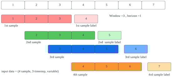
Figure 3. Time series input format.

3.4. LSTM Model Training and Model Evaluation

After the input data has been pre-processed, the LSTM model training will begin, followed by evaluation using the testing data. The evaluation process will involve two stages, namely machine learning evaluation and trading evaluation. In the machine learning evaluation, the prediction accuracy of the LSTM model on the testing data will be computed. Additionally, the predicted result score will be divided into buy (greater than or equal to 0.7), hold (between 0.3 and 0.7), and sell (less than or equal to 0.3). So, if the predicted score is greater than or equal to 0.7, the predicted result will be marked as 1 (recommend to buy); otherwise, it will be marked as 0 (not recommended to buy). In contrast, the trading evaluation will involve evaluating the LSTM model as a trading system, where a “buy” operation will be made if the model predicts an “up” trend at any moment during the testing data, and the return on investment will be calculated. Portfolio evaluation metrics such as cumulative return, Sharpe ratio, and maximum drawdown will be calculated to measure the performance of the proposed model in a stock trading simulation. Additionally, the LSTM model’s trading performance will be compared with the buy-and-hold and optimistic strategies, which are the most fundamental strategies used in the stock market. The buy-and-hold strategy involves buying the stock at the beginning of the testing data period and selling it at the end of the period [23], while the optimistic strategy buys the stock at the current time step and sells it at the next time step if the current stock price is higher than the previous stock price, expecting the stock price to continue to increase in the future. The performance of the proposed model is expected to outperform these two strategies. After the evaluation process, the results, including prediction accuracy and trading simulation performance, will be presented to users. Additionally, by comparing the performance of the proposed model with these two strategies, users can gain a better understanding of the strengths and weaknesses of the model. Figure 4 and Figure 5 illustrate the buy-and-hold and optimistic strategies, respectively.

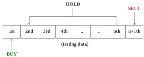
Figure 4. Illustration of the buy-and-hold strategy.

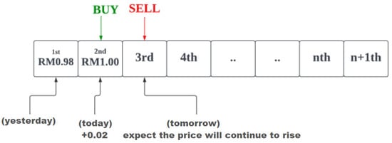
Figure 5. Illustration of an optimistic strategy.

Overall, the proposed model aims to provide reliable predictions and perform better than traditional buy-and-hold and optimistic strategies, as shown through the evaluation process. Algorithm 2 shows the pseudocode of the evaluation process.

Algorithm 2 Pseudocode of the Evaluation Process

var time_step = 2, horizon = 1, npcheck = [],npcheck_percent = [],checksum = 0,

checksum_percent = 0, optimistic = 0, count_operation_done = 0;

var decision_buy = [...y_pred];//computed from Algorithm 3

var actual_close = x_test_new[3].slice(time_step − 1, x_test_new[3].length)

for (let i = 0; i < decision_buy.length; i++) {

if (i + horizon < actual_close.length) {

if (decision_buy[i] == 1) {

count_operation_done++;

checksum += (actual_close[i + horizon]) − (actual_close[i]);

checksum_percent += ((actual_close[i + horizon]) − (actual_close[i]))/

(actual_close[i]);

npcheck.push((actual_close[i + horizon]) − (actual_close[i]));

npcheck_percent.push(((actual_close[i + horizon]) − (actual_close[i]))/

(actual_close[i])); }

if (i − 1 > 0) {

if ((actual_close[i]) > (actual_close[i v 1])) {

optimistic += (actual_close[i + 1]) − (actual_close[i]); } } } }

var avg_return = (checksum/count_operation_done);

var avg_return_percent = (checksum_percent/count_operation_done);

var std_return = getStandardDeviation(npcheck);

var std_return_percent = getStandardDeviation(npcheck_percent);

var sharpe_ratio = (avg_return/std_return) × Math.sqrt(252);

var sharpe_ratio_percent = (avg_return_percent/std_return_percent) × Math.sqrt(252);

var Buy_hold = (actual_close[actual_close.length − 1] − actual_close[0]);

3.5. Fine-Tuning

In this stage, the model training process and model evaluation process will be repeated multiple times with different combinations of indicators as model input so that an architecture design of the LSTM model that works well, in general, can be determined. The model will be further fine-tuned to find out the best hyperparameters, such as the number of time steps, forecast horizon, and decision threshold. After multiple runs of fine-tuning, the optimal model architecture will be determined based on the number of indicators selected by the investor. During the fine-tuning process, a combination of technical indicators that work well will be obtained. The proposed model will rank each of the combinations based on their prediction accuracy.

3.6. System Architecture and Design of the Proposed Stock Prediction Model

The proposed stock prediction model’s system architecture design is illustrated in Figure 6, with the output size of each phase represented by a gray box. The input data will be in the form of a time series, as shown in Figure 3.

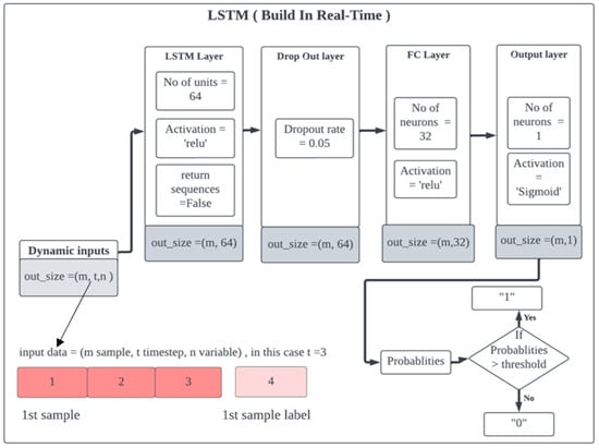
Figure 6. System architecture and design of the stock prediction model.

The model consists of different types of layers, starting with the first hidden layer, which is an LSTM layer with 64 units. The LSTM layer, also known as the RNN layer, will learn the time-series dependency present in the data. Each time step in each input data set will go through all 64 LSTM units, resulting in an output size of (number of samples = m, 64). 64 represents the number of hidden state outputs accumulated from the first-time step to the last time step in each sample.

The activation function used in the LSTM layer is the rectified linear unit (ReLU), which will output the input directly if it is positive; otherwise, it will output zero (see Equation (2)).

$$f\left(x\right)=max\left(0,x\right)$$

(2)

On the other hand, the initial weight of each neuron is assigned using a uniform distribution (see Equation (3)). The a and b are denoted as the minimum value and maximum value, respectively.

$$f\left(x\right)=\frac{1}{\left(b-a\right)}$$

(3)

Next, the data will be passed to the dropout layer, where 5% of the LSTM hidden nodes will be turned off randomly during each training operation to increase the generalization capability of the model and reduce overfitting issues. Finally, the data will be passed to the dense layer with 32 neurons. The purpose of adding a fully connected layer (FC) is to perform classification learning based on the LSTM hidden state data. The activation function used in the LSTM layer is ReLU. The proposed model is an improvement over previous models, which only used the LSTM layer to learn the temporal features and time dependency of the data but did not include any layers for the classification learning.

The output of the dense layer consists of one neuron. The activation function used is a sigmoid function, which will always return a value between 0 and 1, return a value close to zero for a small value, and return a value close to 1 for a large value (see Equation (4)).

$$sigmoid\left(x\right)=\frac{1}{1+e^{-x}}$$

(4)

The proposed LSTM+FC layer model can learn and extract temporal features using the LSTM layer and learn the classification of data using the FC layer. The final output of the model will be in the form of probabilities, and the model will predict the data as “1” if the probability is greater than the threshold and “0” otherwise. The Adam optimizer is used in this training model to update the weight during the training. The set learning rate and epochs for the Adam optimizer are 0.001 and 100, respectively.

The n, y and ŷ are denoted as the number of the data points, the actual label of the data point, and the predicted probability of the data point, respectively. The binary cross-entropy (BCE) method (see Equation (5)) will be used as a loss function to evaluate the predictive and target output values during the training.

$$f\left(x\right)=-\frac{1}{n}\sum _{i=1}^n\left(y_i·\log {\widehat{y}}_i+\left(1-y_i\right)·\log \left(1-{\widehat{y}}_i\right)\right)$$

(5)

The binary accuracy (BA) method (see Equation (6)) will be used as a metric in this LSTM model to calculate the percentage of predicted values that match the actual values of the binary labels.

$$f\left(x\right)=\left\{\begin{array}{c}0,\hspace{1em}\frac{TP+TN}{TP+TN+FP+FN}<0.5\\ 1,\hspace{1em}\frac{TP+TN}{TP+TN+FP+FN}\ge 0.5\end{array}\right.$$

(6)

The true positive (TF), true negative (TN), false positive (FP), and false negative (FN) are denoted as correctly indicating the presence of a condition, correctly indicating the absence of a condition, wrongly indicating a condition is present, and wrongly indicating a condition is absent, respectively. Overall, the proposed stock prediction model is designed to learn from time-series data using LSTM and FC layers, with the aim of accurately predicting the direction of the stock price movement. The model’s output will be probabilities, which can be used to make informed trading decisions. Algorithm 3 shows the pseudocode of the data transformation to a time series.

Algorithm 3 Pseudocode of the Data Transformation to a Time Series

//Creating the LSTM Model

var time_step = 2, horizion = 1;

var x_train_scaled = [];//min max normilzation

const model = tf.sequential();

model.add(tf.layers.lstm({ units: 64, activation: ‘relu’, inputShape: [time_step,

(x_train_new_scaled.length + ind_train_new_scaled.length)], returnSequences: false }))

model.add(tf.layers.dropout({ rate: 0.05 }));

model.add(tf.layers.dense({ units: 32, activation: ‘relu’ }));

model.add(tf.layers.dense({ units: 1, activation: ‘sigmoid’ }));

//Compiling the model

model.compile({

optimizer: tf.train.adam(0.001),

loss: tf.metrics.binaryCrossentropy,

metrics: tf.metrics.binaryAccuracy });

model.fit(x, y, {

batchSize: xtrain.length,

epochs: 100,

verbose: 2

}).then(async(history) => {

var y_hat = [],y_pred = [];

//convert it to array

const values = model.predict(xt).dataSync();

const y_score = Array.from(values);

//today prediction

today.print();

const valuest = model.predict(today).dataSync();

var y_scoret = Array.from(valuest);

y_score.forEach((data, index) => {

if (data >= 0.7) {

y_pred.push(1);

} else {

y_pred.push(0); }

})

const testacc = model.evaluate(xt, yt);

var count_acc_70 = 0;

y_pred.forEach((data, index) => {

if (y_pred[index] == ytest[index]) {

count_acc_70++; }

})

const accuray = [count_acc_70/y_pred.length];

4. Experiments

To evaluate the effectiveness of the proposed model, a simulation was conducted to predict the price movement of 100 stocks between 1 January 2019 and 30 June 2022. The model training data did not include stock data between 1 January 2019 and 30 June 2022, to avoid look-ahead bias and allow the proposed model to make predictions based on unseen data. The evaluation of the proposed model was based on four performance metrics: prediction accuracy, cumulative return, Sharpe ratio, and maximum drawdown. The simulation process also compared the performance of the proposed model strategy with the buy-and-hold strategy, the optimistic strategy, and the prediction method used in a previous article [16], which selected random indicators and applied feature extraction to filter the best-voted features for training. To account for the random initialization of some LSTM algorithm parameters, such as the weight of nodes in each gate, three simulation rounds were conducted per stock to obtain the average accuracy rate and average trading performance. Figure 7 illustrates the simulation procedure for testing the proposed model’s prediction accuracy and trading performance.

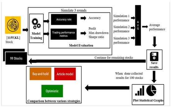
Figure 7. Simulation of the prediction test procedure for the proposed model.

5. Results

5.1. Average Prediction Accuracy Rate Results for the Simulation

After running simulations for all 100 stocks, the results were presented and compared using several performance metrics. Figure 8 displays the average prediction accuracy distribution of the 100 stocks for four different strategies, and Table 3 shows the statistics of the accuracy rate of the 100 stocks for four different strategies.

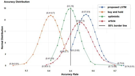
Figure 8. Average accuracy results for 100 stocks for four different strategies.

Table 3. Statistics of the accuracy rate of the 100 stocks for four different strategies.

Strategy	Accuracy Rate
	Mean	Max.	Min.	St. Dev.	Skew.	Kurt.
Proposed model	0.57	0.74	50	0.045	1.29	2.72
Article model	0.54	0.70	39	0.053	−0.06	0.75
Buy-and-hold	0.41	0.48	23	0.045	−1.43	3.04
Optimistic model	0.49	0.72	41	0.039	2.10	10.32

The blue curve represents the proposed model, and each blue dot on the graph represents the average model accuracy of a specific stock. The proposed model achieved at least 50% accuracy for all 100 stocks, which indicates it has passed the first part of the test. Furthermore, the proposed model outperformed the other three strategies, achieving the highest average accuracy rate of around 57%. The prediction approach used in the article [16] obtained an average accuracy of 54% and a minimum accuracy of 39%, which is less than 50%. Therefore, the proposed model is better than the prediction approach used in the article [16]. The buy-and-hold and optimistic strategies achieved significantly lower accuracy rates than the proposed and article models because they lacked statistical analysis. Therefore, machine learning models are expected to outperform these strategies.

5.2. Average Cumulative Return Results for the Simulation

After evaluating the prediction accuracy rate, the proposed model was assessed from a trading perspective. Figure 9 displays the average cumulative return distribution for the 100 stocks under each of the four strategies, along with a summary table, and Table 4 shows the statistics of the cumulative return of the 100 stocks for the four different strategies.

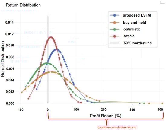
Figure 9. Average cumulative return of 100 stocks for four different strategies.

Table 4. Statistics of the cumulative return of the 100 stocks for four different strategies.

Strategy	Cumulative Return (%)						Number of Stock
	Mean	Max.	Min.	St. Dev.	Skew.	Kurt.	Positive Return	Negative Return
Proposed model	29	372	−40	43.15	3.82	22.94	90	10
Article model	10	119	−70	35.11	0.66	1.32	59	41
Buy-and-hold	12	409	−94	74.16	2.93	12.06	41	59
Optimistic model	−3	343	−80	57.85	2.72	12.48	30	70

The black line in the graph represents the zero cumulative return boundary, where values below it denote a negative cumulative return. Ideally, the graph should skew towards positive returns, indicating profitable trades. As shown in Table 2, 90% of the stocks under the proposed model simulation achieved positive cumulative returns, while the buy-and-hold, optimistic, and article models only had 41%, 30%, and 59% of the stocks with positive returns, respectively. This suggests that the proposed model outperforms the other strategies. Additionally, the proposed model recorded the highest average cumulative return of 29% across the 100 stocks, with the lowest maximum capital losses among the strategies, amounting to only about 40% of profits.

5.3. Average Sharpe Ratio and Maximum Drawdown Results for the Simulation

In addition to accuracy and cumulative return, the proposed model was also evaluated based on risk performance using the Sharpe ratio and maximum drawdown distribution. Figure 10 shows the Sharpe ratio distribution of the 100 stocks, and Table 5 shows the statistics of the Sharpe ratio of the 100 stocks for four different strategies.

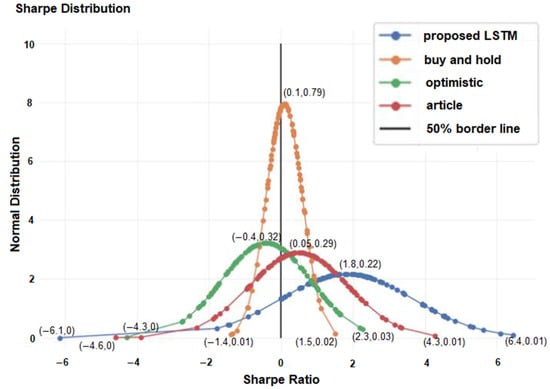
Figure 10. Average Sharpe ratio of 100 stocks for four different strategies.

Table 5. Statistics of the Sharpe ratio of the 100 stocks for four different strategies.

Strategy	Sharpe Ratio
	Mean	Max.	Min.	St. Dev.	Skew.	Kurt.
Proposed model	1.83	6.44	−6.14	0.045	−0.40	2.88
Article model	0.49	4.27	−4.58	0.053	−0.42	2.08
Buy-and-hold	0.09	1.51	−1.38	0.045	−0.29	1.10
Optimistic model	−0.41	2.27	−4.28	0.039	−0.15	−0.12

It indicates that the proposed model outperformed the other strategies, achieving a high Sharpe ratio value of 1.83. Figure 11 shows the maximum drawdown distribution, and Table 6 shows the statistic of the maximum drawdown of the 100 stocks for four different strategies.

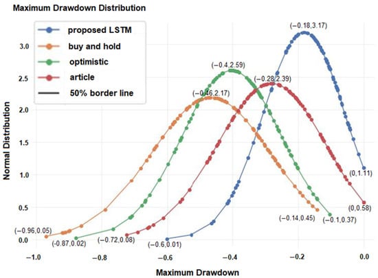
Figure 11. Average maximum drawdown of 100 stocks for four different strategies.

Table 6. Statistics of the maximum drawdown of the 100 stocks for four different strategies.

Strategy	Maximum Drawdown
	Mean	Max.	Min.	St. Dev.	Skew.	Kurt.
Proposed model	−0.18	−0.60	0.00	0.045	−1.07	0.68
Article model	−0.28	−0.72	0.00	0.053	−0.55	−0.14
Buy-and-hold	−0.46	−0.96	−0.14	0.045	−0.72	0.46
Optimistic model	−0.40	−0.87	−0.10	0.039	−0.53	0.10

It indicates that the proposed model is the least risky strategy, with an average maximum drawdown value of around −0.18 (−18%). Overall, the results indicate that the proposed model is the most reliable and effective strategy compared to the buy-and-hold, optimistic, and article models, with high accuracy, a positive cumulative return, a high Sharpe ratio, and low maximum drawdown values. These results demonstrate the potential of the proposed model for predicting stock prices and supporting trading decisions.

6. Discussion

The simulation results indicate that the proposed model is superior to the prediction approach used by the previous work’s method, which randomly selected technical indicators. The proposed model achieved the highest average prediction accuracy among the strategies, around 57%, with a maximum accuracy of around 74%. While 57% may not seem satisfactory, it is difficult to evaluate the model’s success based on prediction accuracy alone, as it can still achieve a higher investment return if the capital gains from correct predictions are higher than the capital losses from incorrect predictions. Therefore, the proposed model was also evaluated as a trading system using a trading simulation.

The overall portfolio performance comparison between the four strategies shows that the proposed model is the best strategy. It achieved the highest average cumulative return of around 29% across 100 stocks, with a positive cumulative return for 90 stocks, outperforming the previous work’s approach. This is clear evidence that the proposed model can detect the stock movement that leads to high returns. The proposed method also has the lowest risk as measured by the Sharpe ratio and the maximum drawdown. The Sharpe ratio of 1.83 indicates a return of 1.83% per unit of risk taken, while the maximum drawdown of only −18% indicates that the proposed method and strategy experienced the lowest risk in history. Table 7 shows the comparison of the experiment results among the related works and the proposed model.

Table 7. Comparison of the experiment results among the related works and the proposed model.

Article	Methods	Dataset	Element	Train, Validate and Test Data Ratio	Dataset Records	Accuracy
[16]	SVM	3 Indian stocks	6 technical indicators	N/A	2 years	52.03%
	Logistic regression					52.98%
	Embedded layer LSTM					55.53%
	Optimal LSTM					59.26%
[9]	ANN	Technical indicators and fundamental indicators S&P 500 Index ETF (SPY) return	60 financial and economical features	70%:15%:15%	377 days	58.1%
[24]	ANN	25 Colombian Stocks	9 technical indicators	75%:0%:25%	372 days	76%
	SVM					78%
[25]	Tf-idf algorithm feature extraction + SVM	AAPL on S&P 500	5 fundamental and 4 technical indicators	80%:0%:20%	1467 days	49.17%
	joint learning feature extraction + SVM					54.92%
	CNN feature extraction + SVM					45.60%
	CNN feature extraction + LSTM					51.32%
	joint learning feature extraction + LSTM					55.44%
[26]	Decision Tree	NIFTY 50 Indian stock market index	75 technical indicators	70%:0%:30%	4977 days	75.08%
	Naïve Bayes					71.26%
	Multi-Layer Perceptron					76.02%
	Random Forest					80.44%
	SVM					78.63%
	History Bits					87.36%
Proposed model	LSTM	100 Bursa Malaysia stocks	22 technical indicators	70%:0%:30%	>3000days (depend on the stock listing date)	57%

According to the article model, the average accuracy among the support vector machine, logistic regression, embedded layer LSTM, and optimal LSTM models (article model) is 52.03%, 52.98%, 55.53%, and 59.26%, respectively, using the three Indian stocks [16]. However, the average accuracy of the article model is 41% using 100 stocks in Malaysia, which is 17% lower compared to the article result. On the other hand, the average accuracy of the proposed model is greater than that of the support vector machine, logistic regression, and embedded layer LSTM in the article [16]. In addition, the proposed method has a better performance compared to the CNN + LSTM model and joint learning + LSTM model in article [25], which obtained 51.32% and 55.44%, respectively, of the prediction accuracy. Other than LSTM algorithms, such as ANN, SVM, random forest, etc., in articles [24,26], greater than 70% prediction accuracy was obtained, which is far better than the LSTM performance result.

In conclusion, the proposed model is an effective approach for stock prediction and trading, with superior performance compared to other strategies. It achieved high prediction accuracy and high investment returns while minimizing risks. The simulation results validate the proposed model’s effectiveness in predicting and trading stocks, making it a promising tool for investors and traders in the stock market.

7. Conclusions

In conclusion, this study has provided evidence that involving investors in the data input process can lead to more meaningful stock predictions and trading strategies. By integrating domain knowledge with machine learning techniques, such as the LSTM algorithm, the proposed approach achieved superior results compared to the previous work’s approach of randomly selecting technical indicators. The higher average prediction accuracy, cumulative return, and lower trading risk demonstrated the effectiveness of this approach in detecting stock movements that lead to high returns.

This study highlights the importance of incorporating domain knowledge and the limitations of relying solely on machine learning techniques. Randomly selecting technical indicators as input data could introduce noise and overlook significant indicators, leading to suboptimal performance. Therefore, this approach has the potential to improve the accuracy of prediction models in other domains that require domain knowledge and expertise.

The limitation of this study is that it only performed well in bullish stocks but not in bearish stocks. Therefore, we aimed to investigate and improve the model so that it can generalize well to all stocks, regardless of their future state. On the other hand, this study only tested 100 Malaysian stocks with historical data and 22 technical indicators. The proposed model can be further studied using remaining Malaysian and foreign stocks with additional fundamental indicators, sentiment analysis (e.g., financial news), the gross domestic product index, etc. In this study, prediction accuracy and accumulative return profit are used as evaluation metrics. However, this study does not cover the root-mean-square deviation, mean absolute percentage error, median absolute error, precision, receiver-operating characteristic analysis, etc. Therefore, those metrics should be covered in future studies.

Future studies could further improve the proposed model by allowing investors to customize fundamental indicators such as the PE ratio and EPS. This would provide additional domain knowledge and increase the model’s accuracy in detecting significant movements in the stock market. Additionally, future research could explore the use of other machine learning techniques and their potential integration with domain knowledge to further improve stock prediction and trading strategies.

References

- Sawale, G.J.; Rawat, M.K. Stock Market Prediction using Sentiment Analysis and Machine Learning Approach. In Proceedings of the 2022 4th International Conference on Smart Systems and Inventive Technology, Tirunelveli, India, 20–22 January 2022. [Google Scholar]
- Li, L.; Wu, Y.; Ou, Y.; Li, Q.; Zhou, Y.; Chen, D. Research on machine learning algorithms and feature extraction for Time Series. In Proceedings of the 2017 IEEE 28th Annual International Symposium on Personal, Indoor, and Mobile Radio Communications, Montreal, QC, Canada, 8–13 October 2017. [Google Scholar]
- Wu, T.-Y.; Li, H.; Chu, S.C. CPPE: An Improved Phasmatodea Population Evolution Algorithm with Chaotic Maps. Mathematics 2023, 11, 1977. [Google Scholar]
- Chhajer, P.; Shah, M.; Kshirsagar, A. The applications of artificial neural networks, support vector machines, and long–short term memory for stock market prediction. Decis. Anal. J. 2022, 2, 100015. [Google Scholar] [CrossRef]
- Wu, M.-E.; Syu, J.-H.; Chen, C.-M. Kelly-based options trading strategies on settlement date via supervised learning algorithms. Comput. Econ. 2022, 59, 1627–1644. [Google Scholar] [CrossRef]
- Sezer, O.B.; Ozbayoglu, M.; Dogdu, E. A deep neural-network based stock trading system based on evolutionary optimized technical analysis parameters. Procedia Comput. Sci. 2017, 114, 473–480. [Google Scholar] [CrossRef]
- Naik, R.L.; Ramesh, D.; Manjula, B.; Govardhan, A. Prediction of Stock Market Index Using Genetic Algorithm. Comput. Sci. Inf. Syst. 2012, 3, 162–171. [Google Scholar]
- Nti, I.K.; Adekoya, A.F.; Weyori, B.A. A systematic review of fundamental and technical analysis of stock market predictions. Artif. Intell. Rev. 2019, 53, 3007–3057. [Google Scholar] [CrossRef]
- Zhong, X.; Enke, D. A comprehensive cluster and classification mining procedure for Daily Stock Market Return Forecasting. Neurocomputing 2017, 267, 152–168. [Google Scholar] [CrossRef]
- Picasso, A.; Merello, S.; Ma, Y.; Oneto, L.; Cambria, E. Technical analysis and sentiment embeddings for market trend prediction. Expert Syst. Appl. 2019, 135, 60–70. [Google Scholar] [CrossRef]
- Kader, A.; Izzati, N. A Review of Long Short-Term Memory Approach for Time Series Analysis and Forecasting. In Proceedings of the 2nd International Conference on Emerging Technologies and Intelligent Systems, 2–3 September 2022. [Google Scholar]
- Kumar, S.; Damaraju, A.; Kumar, A.; Kumari, S.; Chen, C.-M. LSTM Network for Transportation Mode Detection. J. Internet Technol. 2021, 22, 891–902. [Google Scholar] [CrossRef]
- Moghar, A.; Hamiche, M. Stock market prediction using LSTM recurrent neural network. Procedia Comput. Sci. 2020, 170, 1168–1173. [Google Scholar] [CrossRef]
- Understanding LSTM Networks. Available online: https://colah.github.io/posts/2015-08-Understanding-LSTMs/ (accessed on 23 May 2023).
- Zhang, S.M.; Su, X.; Jiang, X.-H.; Chen, M.L.; Wu, T.Y. A traffic prediction method of bicycle-sharing based on long and short term memory network. J. Netw. Intel. 2019, 4, 17–29. [Google Scholar]
- Agrawal, M.; Khan, A.U.; Shukla, P.K. Stock Price Prediction using Technical Indicators: A Predictive Model using Optimal Deep Learning. Int. J. Recent Technol. Eng. 2019, 8, 2297–2305. [Google Scholar] [CrossRef]
- Gao, P.; Zhang, R.; Yang, X. The application of stock index price prediction with neural network. Math. Comput. Appl. 2020, 3, 53. [Google Scholar] [CrossRef]
- Joiner, D.; Vezeau, A.; Wong, A.; Hains, G.; Khmelevsky, Y. Algorithmic Trading and Short-term Forecast for Financial Time Series with Machine Learning Models; State of the Art and Perspectives. In Proceedings of the 2022 IEEE International Conference on Recent Advances in Systems Science and Engineering, Tainan, Taiwan, 7–10 November 2022. [Google Scholar]
- Kurani, A.; Doshi, P.; Vakharia, A.; Shah, M. A Comprehensive Comparative Study of Artificial Neural Network (ANN) and Support Vector Machines (SVM) on Stock Forecasting. Ann. Data Sci. 2023, 10, 183–208. [Google Scholar] [CrossRef]
- Hu, Z.; Zhao, Y.; Matloob, K. A Survey of Forex and Stock Price Prediction Using Deep Learning. Appl. Syst. Innov. 2021, 4, 9. [Google Scholar] [CrossRef]
- Sheth, D.; Shah, M. Predicting stock market using machine learning: Best and accurate way to know future stock prices. Int. J. Syst. Assur. Eng. Manag. 2023, 14, 1–18. [Google Scholar] [CrossRef]
- Weckman, G.; Lakshminarayanan, S. Identifying Technical Indicators for Stock Market Prediction with Neural Networks. In Proceedings of the IIE Annual Conference, Houston, TX, USA, 15–19 May 2004. [Google Scholar]
- Nelson, D.M.; Pereira, A.C.; de Oliveira, R.A. Stock market’s price movement prediction with LSTM neural networks. In Proceedings of the 2017 International Joint Conference on Neural Networks, Anchorage, AK, USA, 14–19 May 2017. [Google Scholar]
- Bustos, O.; Pomares, A.; Gonzalez, E. A comparison between SVM and multilayer perceptron in predicting an emerging financial market: Colombian stock market 2017. In Proceedings of the 2017 Congreso Internacional de Innovacion y Tendencias en Ingenieria, Bogota, Colombia, 4–6 October 2017. [Google Scholar]
- Liu, Y.; Zeng, Q.; Yang, H.; Carrio, A. Stock Price Movement Prediction from Financial News with Deep Learning and Knowledge Graph Embedding. In Proceedings of the 15th Pacific Rim Knowledge Acquisition Workshop, Nanjing, China, 28–29 August 2018; pp. 102–113. [Google Scholar]
- Sakhare, N.N.; Shaik, I.S.; Saha, S. Prediction of stock market movement via technical analysis of stock data stored on blockchain using novel History Bits based machine learning algorithm. IET Softw. 2022. [Google Scholar] [CrossRef]
Disclaimer/Publisher’s Note: The statements, opinions and data contained in all publications are solely those of the individual author(s) and contributor(s) and not of MDPI and/or the editor(s). MDPI and/or the editor(s) disclaim responsibility for any injury to people or property resulting from any ideas, methods, instructions or products referred to in the content. |
© 2023 by the authors. Licensee MDPI, Basel, Switzerland. This article is an open access article distributed under the terms and conditions of the Creative Commons Attribution (CC BY) license (https://creativecommons.org/licenses/by/4.0/).