Article

Intrusion Detection in Networks by Wasserstein Enabled Many-Objective Evolutionary Algorithms

by
Andrea Ponti
1,2,*,
Antonio Candelieri
1,
Ilaria Giordani
3,4 and
Francesco Archetti
2,3
1
Department of Economics, Management and Statistics, University of Milano-Bicocca, 20126 Milan, Italy
2
Consorzio Milano Ricerche, 20125 Milan, Italy
3
Department of Computer Science, Systems and Communication, University of Milano-Bicocca, 20126 Milan, Italy
4
Oaks S.R.L., 20125 Milan, Italy
*
Author to whom correspondence should be addressed.
Mathematics 2023, 11(10), 2342; https://doi.org/10.3390/math11102342
Submission received: 29 March 2023 / Revised: 10 May 2023 / Accepted: 16 May 2023 / Published: 17 May 2023
(This article belongs to the Special Issue Combinatorial Optimization and Applications)

Abstract

:
This manuscript explores the problem of deploying sensors in networks to detect intrusions as effectively as possible. In water distribution networks, intrusions can cause a spread of contaminants over the whole network; we are searching for locations for where to install sensors in order to detect intrusion contaminations as early as possible. Monitoring epidemics can also be modelled into this framework. Given a network of interactions between people, we want to identify which “small” set of people to monitor in order to enable early outbreak detection. In the domain of the Web, bloggers publish posts and refer to other bloggers using hyperlinks. Sensors are a set of blogs that catch links to most of the stories that propagate over the blogosphere. In the sensor placement problem, we have to manage a trade-off between different objectives. To solve the resulting multi-objective optimization problem, we use a multi-objective evolutionary algorithm based on the Tchebycheff scalarization (MOEA/D). The key contribution of this paper is to interpret the weight vectors in the scalarization as probability measures. This allows us to use the Wasserstein distance to drive their selection instead of the Euclidean distance. This approach results not only in a new algorithm (MOEA/D/W) with better computational results than standard MOEA/D but also in a new design approach that can be generalized to other evolutionary algorithms.

1. Introduction

1.1. Motivations

In the current manuscript, we explore the general problem of detecting outbreaks in networks, where we are given, or obtain through simulation, a representation of a dynamic process propagating over the network, and we want to select a set of nodes at which to deploy sensors in order to monitor the propagation process and detect the outbreak/intrusion as early and effectively as possible.
In water distribution networks (WDNs), accidental or malicious intrusions can cause contaminants to spread over the network: the decision we face is the selection of locations of sensors to detect these contaminations as quickly as possible. Epidemic scenarios also fit into this setting: given a network of interacting people, our problem is to choose a small set of people whose surveillance enables the early detection of any disease outbreak, when very few people are already infected [1,2]. In the domain of Web, bloggers publish posts and use hyperlinks to other content on the web: we want to select a set of blogs to links to most of the stories that propagate over the blogosphere [3,4]. In outbreak detection, there are different criteria one may want to optimize. The main is the time to detect a cascade or the spreading of contaminated water; another could be to minimize the population affected by the outbreak.
In this paper, we focus on the problem of optimal sensor placement (OSP) for contaminant detection in WDNs, which is a major concern for citizens and governments alike. Indeed, the WDN is the most vulnerable module in a water supply and distribution system due to the large number of unprotected access points. An effective placement of sensors is a key element in a contamination warning system, both for budgetary and technical reasons, which constrain the number of sensors and their locations. The sensor placement is also a critical element in the detection and localization of water leaks, which in turn impact the quantity of lost water and energy consumption in network operations. There are several objectives making sensor placement a multi-objective problem (MOP). In MOPs, there is not a unique solution but a set of solutions, each representing a trade-off between different objectives, which is expressed by the notion of dominance. The solution representing the optimal (non-dominated) trade-offs is the Pareto set, whose image in the objective space is the Pareto front.
In the present paper, we describe a mixed integer programming formulation for sensor placement in WDNs that incorporates the dynamics of contamination events from simulation models and is represented as a time series of contaminant concentrations. These time series are used to estimate the detection time at different sensors and the volume of contaminated water.
Even for cheap objective functions, locating the complete Pareto set may not be possible: the OSP problem is NP-hard, requiring efficient approximate methods, as evolutionary algorithms, to generate a good approximation of the Pareto set. The authors believe that considering only the average value of the objective function over all the scenarios does not correctly capture the “risk” elements of the placement. Therefore, we propose using the standard deviation of the objective function as a companion objective. The evaluation of the objective functions is expensive due to the simulation of multiple contamination events. Simulating the contaminant propagation allows us to compute both the average minimum detection time related to the placement of sensors and its standard deviation. Two more objectives considered in the current paper are the amount of water consumed before detection and its standard deviation.
Among the heuristics to solve multi-objective optimization problems, evolutionary algorithms have shown particular versatility and efficiency. There are two main strategies in the design of multi-objective evolutionary algorithms (MOEAs): (i) Pareto-based evolving populations of possible solutions, comparing and ranking them according to Pareto dominance [5]; (ii) decomposition-based [6], whose basic idea is to decompose MOPs, through aggregating functions, into several single objective problems and optimize them simultaneously in a collaborative manner. Since the optimal solution of each subproblem is proved to be Pareto optimal, the collection of optimal solutions obtained by varying the aggregation parameters can be considered a good approximation of the Pareto set. The key problem in many-objective problems (i.e., with more than two objectives) is that the number of incomparable solutions dominates the population, reducing the selection pressure and leading to poor convergence to the Pareto front. It is also more difficult to preserve diversity in the solution set.
The algorithm proposed in this paper, MOEA/D/W, is built upon the Pymoo implementation of the MOEA/D algorithm. MOEA/D decomposes the multi-objective into single-objective problems associated with an aggregation weight vector. The scalarized problems are solved with a single-objective algorithm, and the set of their solutions represents an approximation of the Pareto Set (Front). There are two basic design decisions: the scalarizing function (linear or Tchebycheff are the most common, but others are possible) and the choice of aggregation vectors. The key contribution of this paper is to interpret the weight vectors as probability measures and, in particular, as points in the unit simplex since they are always positive, and they all sum to one. This allows us to use the Wasserstein distance between the weight vectors instead of the Euclidean distance.
The Wasserstein distance, also known as the optimal transport distance, is a mathematically principled method to align probability distributions. Originated by a paper by Monge [7], it received its linear programming formulation in Kantorovich [8]. A complete mathematical formulation is presented in [9], while [10] offers a complete review of the recent theoretical and computational advances. Notably, it has found applications in machine learning from shape analysis to image interpolation, domain adaptation [11], parameter estimation in simulation models [12], structured data on graphs [13], active learning [14] and adversarial networks [15]. The optimal transport distance has many important properties.
The key research question addressed in the present paper is whether the computational efficiency of a MOEA/D algorithm can be improved using Wasserstein-enabled operators and whether this improvement increases with the number of objectives.

1.2. Contributions

  • The contributions of this paper are listed below.
  • A risk-aware optimal sensor placement model.
  • A many-objective optimization formalization of the optimal sensor placement problem, where the objectives are the mean and the standard deviation of the detection time over a set of simulated contamination events along with the amount of contaminated water consumed before detection and its variance.
  • The representation of the weights in the decomposition as discrete probability distributions whose distance is computed by the Wasserstein distance.
  • The formulation of a Wasserstein enabled selection of the weight parameters in the scalarization.
  • A set of computational results, for standard benchmark problems and a real-world application, which demonstrates that MOEA/D/W has a significant performance improvement over MOEA/D.

1.3. Organization of the Paper

Section 2 provides a short presentation of related works. Section 3 introduces the Wasserstein distance. Section 4 analyzes the optimal sensors’ placement problem and the evaluation of the objective functions. Section 5 describes the proposed algorithm MOEA/D/W. Section 6 presents the setting of computational experiments and their results. Section 7 contains concluding remarks.

2. Related Works

In the previous section, we briefly introduced the issue of sensor placements, multi-objective evolutionary algorithms, and the Wasserstein distance; here, we provide a more specific analysis of related works.
A closely related paper is [16]. Its novelty was to consider optimal sensor placement as a simulation optimization problem and sensor placements as a discrete probability distribution, which are specifically considered as histograms. The algorithm proposed, MOEA/WST, is based on the Pareto sampling strategy and built on NSGA-II. The selection of the parents for the next generation was performed on the basis of the Wasserstein distance.
The novelty of the current paper over the previous one (Ponti et al., 2021) is given by several factors:
  • The number of objectives has been augmented from 2 (mean detection time and its standard deviation) to 4, including the mean amount of water consumed and its standard deviation.
  • While the paper [16] was focused on the Pareto sampling strategy of non-dominated sorting, the current paper is based on decomposition, which is usually held to be higher performing for many-objective problems.
  • This has required a new strategy to map the MOEA/D algorithm into the Wasserstein base MOEA/D/W.
  • The set of test functions has been substantially augmented including DTLZ2.
Significant papers are: [17], where a regret-based scalarization function based on the Tchebysheff distance in the NSGA-II framework is introduced for the optimal sensor placement; [18], which considers jointly both leak localization and sensor placement; and [19], whose approach is risk based. Another Pareto-based approach is proposed in [20], where the inclusion of individuals in the approximate Pareto set is decided according to their contribution to the improvement of the hypervolume.
Another related paper to ours is [21], in which the objectives are the number of sensors and the risk of contamination. The algorithm NSGA-II is used to solve the multi-objective problem. These papers show several advantages of MOEAs for solving the multi-objective optimal sensor placement problem. A drawback of MOEAs is their relatively low sample efficiency, which might become a problem given the size of real-world optimal sensor placement problems. A solution proposed in the literature to mitigate this problem is the development of problem-specific operators. In [22,23], a population-based algorithm is endowed with problem-specific recombination and repair operators, while in [24], new crossover operators and mutation probabilities based on the hypervolume improvement are proposed. The issue of comparing and evaluating solution sets provided by different algorithms has been extensively analyzed in [25]. Another approach integrates with EAs probabilistic models given by Gaussian processes. The first contributions along this research line are ParEGO [26] and MOEA/D with Gaussian processes [27] and, more recently, [28].
The contribution of this paper can be seen as a proposal of a general problem-agnostic approach to improving the efficiency of MOEAs embedding part of the optimization process in a space of distributions. Even if the sensor placement problem has been mostly addressed by EAs, methods from mathematical programming have also been considered [29,30].
A graph variant of the Wasserstein distance is called the Gromow–Wasserstein (GW) distance, whose use was first advocated in [31]. The issue of graph partitioning and matching is addressed in [32]. Given two graphs, the optimal transport map associated with their GW distance provides the correspondence between their nodes and achieves graph matching. The same approach is proposed in [33] for clustering. Another topic addressed with optimal transport is learning on graphs. An early paper is [34], where the label associated with a node is not a scalar but a probability distribution, for instance, the pressure at a node in a WDN can be seen as a discrete distribution over the 24 h cycle. Pressure values can be known only where there are sensors. Their measurements need to be propagated to the entire network. The Wasserstein distance is used to propagate their measurements to the whole network, generating a distribution-valued map. Another learning context to learn over graphs is the graphon, which is defined in an infinite dimensional space and represents arbitrarily sized graphs. Given a set of graphs generated by an underlying graphon, the GW distance is used in [35] to learn an approximation of the underlying graphon. The above papers about WST on graphs are considered for completeness, even if their applications are beyond the scope of the current paper and will be considered in future activities.

3. The Probability Simplex and the Wasserstein Space

A discrete measure α is defined by a η -dimensional vector a —whose elements are the so-called weights—and a set of associated locations (i.e., support) x 1 , ,   x η Γ q :
α = i = 1 η a i δ x i
with δ x i the Dirac function centred at x i . The discrete measure α is a (positive) probability measure if the vector a belongs to the probability simplex Σ η (i.e., it is a probability vector), which is defined as follows:
Σ η = u + η : i = 1 η u i = 1
The Wasserstein (WST) distance between two distributions α 1 , α 2 Σ η is the solution of the following linear program:
W α 1 , α 2 = min γ i j + i I 1 ,   j I 2 γ i j   d x i 1 , x j 2
The transport cost between x i 1 and x j 2 , d x i 1 , x j 2 is usually assumed to be the p -th power of the norm || x i 1 ,   x j 2 || (usually the Euclidean distance). Two index sets I 1 = 1 , , m 1 and I 2 are used to define Equations (4) and (5), which represent the in-flow and out-flow constraint:
i I 1 γ i j = a j 2 ,   j I 2
j I 2 γ i j = a i 1 ,   i I 1
where a i and a j are defined in Equation (1). The terms γ i j are called matching weights between support points x i 1 and x j 2 or the optimal coupling for α 1 and α 2 . Discrete optimal transport is a linear program and thus can be solved exactly in O n 3 log n with interior point methods. The computation of the Wasserstein distance is the solution of a minimum cost flow problem on a bi-partite graph in which the support points of α 1 ( α 2 ) are, respectively, the sources and the sinks, while the weight of edges between sources and sinks are the transportation costs. In the case of one-dimensional discrete distributions, the computation of the Wasserstein distance reduces to a simple sorting and the application of the following closed formula:
W p α 1 , α 2 = 1 n i n x i 1 x i 2 p 1 p
where x i 1 and x i 2 are the supports of the distributions α 1 and α 2 and x i 1 and x i 2 are the sorted samples.

4. Problem Formulation

4.1. Multi-Objective Optimization

The general formulation of the multi-objective optimization problem can be stated as:
min x Ω d F x = f 1 x , , f m x
where multiple objectives have to be simultaneously optimized. It is important to note that these objectives may be in contrast with each other, meaning that an improvement in one objective could compromise the others. Consider that two points, x k , x h d , F x k , are said to dominate F x h iff f i x k f i x h     i = 1 , , m and f j x k > f j x h for at least an index j = 1 , , m . There is not one optimal solution in multi-objective optimizations; instead, the goal is to find the set of non-dominated solutions, i.e., the Pareto set. The image of the Pareto set, i.e., the set of all non-dominated objective vectors, is called the Pareto front. All the points x having the associated F x on the Pareto front represent the best trade-offs between the conflicting objectives. Figure 1 shows an example of the Pareto set and the corresponding Pareto front.
The quality evaluation of Pareto solutions is a non-trivial issue in multi-objective optimizations. A widely used metric is the hypervolume indicator, which measures the volume between a non-dominated set and a fixed reference point in the objective space.

4.2. Optimal Sensor Placement

The optimal sensor placement (OSP) problem aims to identify the best position of a fixed number n s of sensors with the goal to optimize an impact measure. In particular, we consider the problem of detecting contaminations.
Consider a water distribution network modelled as a graph G = V , E . We assume that sensors can be placed in a subset of the nodes L V and that they are capable of detecting contaminants at any concentration level. In addition, we also assume that when a contaminant intrusion is first detected, all further consumption is prevented. Thus, a sensor placement is represented as a binary vector s 0 , 1 L where s i = 1 if a sensor is located at node i , and s i = 0 otherwise. Then, we assume that contaminant can be injected in a subset of nodes A V .
We introduce a general formulation of OSP as a multi-objective optimization problem. Let d a i be a general “impact” of a sensor located at node i when a contaminant is introduced in node a , then the OSP problem is:
min f 1 s = a A 1 A i = 1 , . . , L d a i x a i s . t . i = 1 , . . , L s i n s s i 0 , 1
where x a i is an indicator variable that assumes value x a i = 1 if s i = 1 is the first sensor in the placement to detect the contamination injected in node a , and x a i = 0 otherwise. Here, f 1 is the average of an impact measure. In addition, as a measure of risk, we consider its standard deviation as a second objective:
f 2 s = 1 A a A i = 1 , . . , L d a i x a i f 1 s 2
The impact measures considered in this are the detection time and the volume of contaminated water; in the two-objective formulation, the objectives are the average detection time and its standard deviation; in the four-objective formulation, we have also considered the average volume of contaminated water and its standard deviation.
The above sensor placement model is identical to the well-known p -median facility location problem in which n s facilities are to be located on m potential sites such that the sum of distances d a j between each of the n customers and the nearest facility is minimized.

4.3. Simulation and Event Data Description

To analyze the spread of the contaminant through the WDN, many simulations have been performed using the WNTR [36] package, which is a Python wrapper of the widely used EPANET simulator. In particular, a simulation for each contamination event (i.e., injection points of the contaminant) has been executed, tracking the contaminant concentration at each node of the network. Each simulation has been performed for 24 h, with a simulation step of 1 h. The structure of the data generated in the simulation is analysed in [37].
Assuming that a sensor, located in a node, detects the contamination if the concentration of contaminant at the node exceeds a given threshold τ , we can associate a discrete probability distribution of the detection times over different contamination events to each sensor. Consider a sensor placed at node i ; for each contamination event a A , we register the detection time t a i , i.e., the time when the concentration of contaminants exceeds τ .

5. Wasserstein-Enabled Multi-Objective Evolutionary Algorithm

MOEA/D is a multi-objective evolutionary algorithm based on the decomposition strategy proposed in [6]. The idea of MOEA/D is to decompose the multi-objective problem into N single-objective problems; the solution of each of these problems results in a non-dominated point.
There are several strategies to scalarize the multi-objective problem. Consider a set of m -dimensional weight vectors λ 1 , , λ N and a reference point z . The simpler approach is the linear scalarization of the objectives, but it can result in a poor approximation of the Pareto front, especially when dealing with a non-convex Pareto front. A more effective approach is the Tchebycheff decomposition in which the objective function of the j -th single-objective subproblems is:
g t e x | λ j , z = max 1 i m λ i j f i x z i
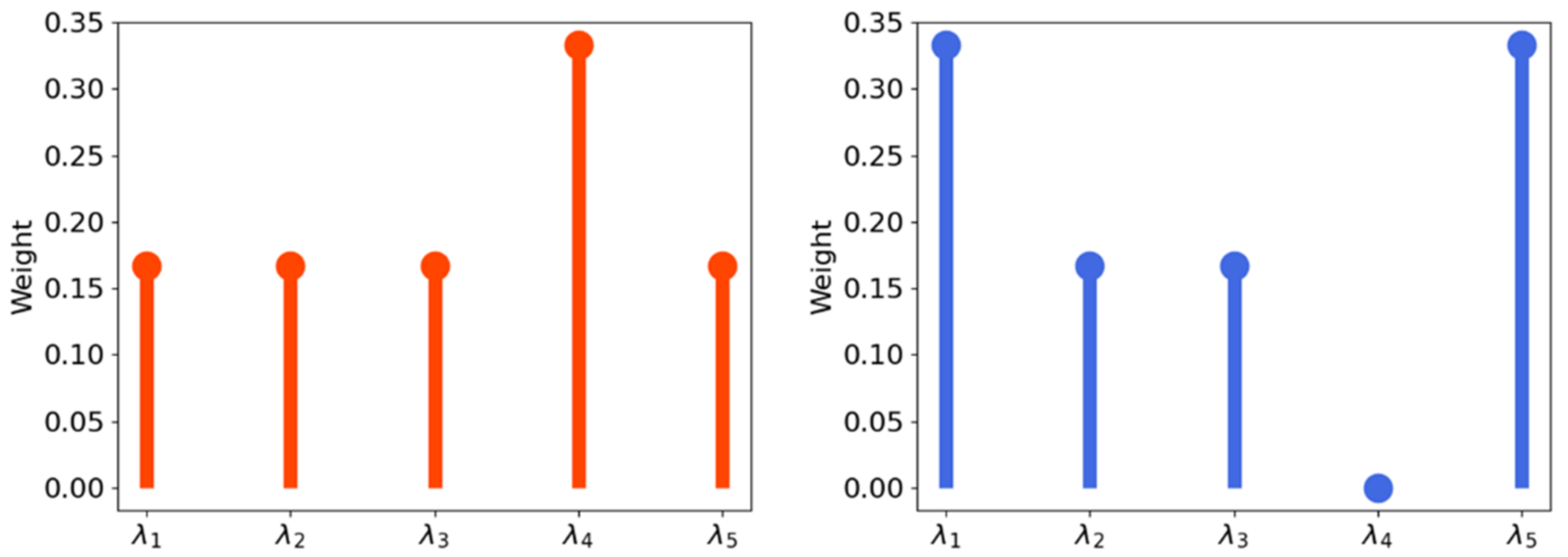
The key element of the proposed algorithm, namely MOEA/D/W, is the interpretation of the weight vectors λ i as probability measures and in particular as points in the simplex (Figure 2), since they are always positive, and they all sum to one.
In the standard implementation of MOEA/D, the Euclidean distance between any two weight vectors is computed, then the neighborhood of each weight vector i = 1 , , N is the set B i = i 1 , , i T , where λ i 1 , , λ i T are the T closest weight vectors to λ i . In MOEA/D/W, the Wasserstein distance between the weight vectors is used instead of the Euclidean distance. Now, the neighbourhood of each weight vector B W i is built using the T farthest vectors, in the Wasserstein sense, from λ i . Then, both MOEA/D and MOEA/D/W randomly select two indexes k , l from B i and B W i , respectively, and then generate a new solution y from x k and x l by using genetic operators (crossover and mutation). This process is repeated until a termination criterion is satisfied, such as the number of generations or the number of function evaluations.
A key factor in decomposition-based MOEA is the initialization of the weight vectors which define the subproblems. In this paper, Das and Dennis’s approach [38] has been used, in which a set of weight vectors λ 1 , λ N is sampled from a unit simplex where N = p m + 1 m 1 . The N weight vectors are uniformly spaced by 1 p , where p is the number of partitions considered along each objective. For a fair comparison, the same crossover and mutation operators have been considered for both MOEA/D and MOEA/D/W. In particular, the simulated binary crossover with a probability of 1 and η = 20 and the polynomial mutation with a probability of 0.9 and η = 20 have been used.

6. Computational Results

6.1. Experimental Setting

We have evaluated our approach in two different settings.
First, we have considered a widely used set of benchmark multi-objective problems, namely DTLZ2, which is defined as:
min f 1 x = 1 + g x 1 : k cos x 1 π / 2 cos x m 2 π / 2 cos x m 1 π / 2 min f 2 x = 1 + g x 1 : k cos x 1 π / 2 cos x m 2 π / 2 sin x m 1 π / 2 min f 3 x = 1 + g x 1 : k cos x 1 π / 2 sin x m 2 π / 2 min f m x = 1 + g x 1 : k sin x 1 π / 2 with   g x 1 : k = i = 1 k x i 0.5 2 0 x i 1 ,         for i = 1 , , n
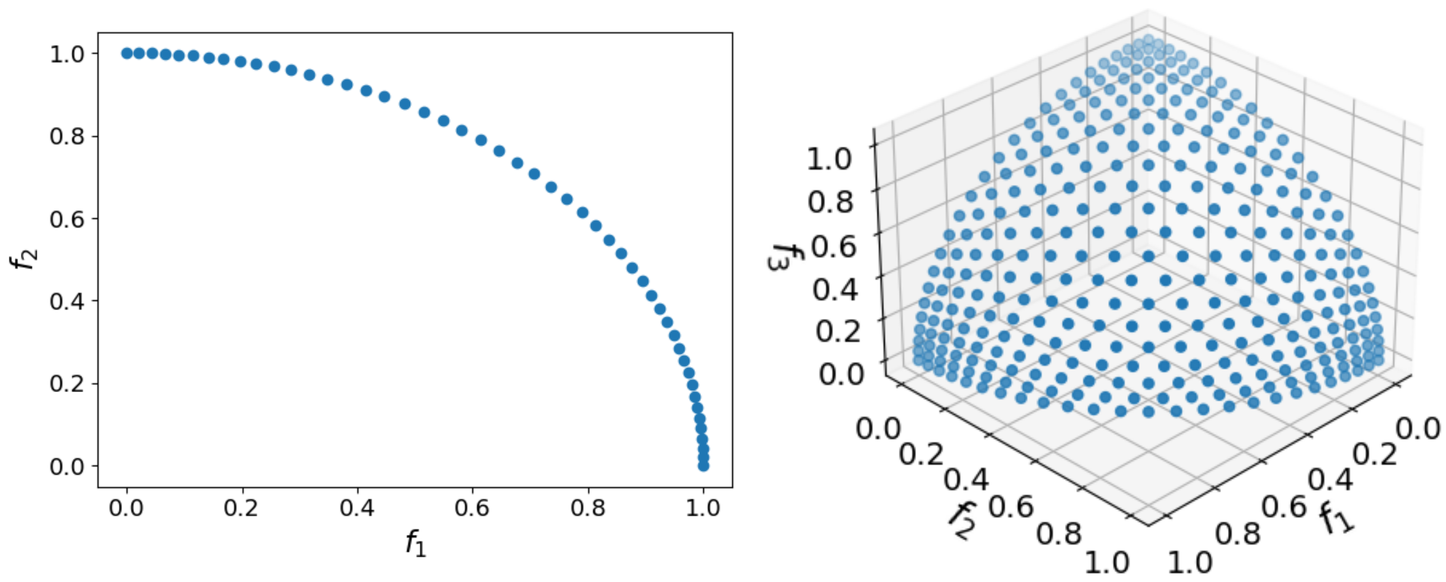
with k = n m + 1 . This function is often used to investigate a MOEA’s ability to scale up its performance in a large number of objectives. The Pareto-optimal solutions correspond to x 1 : k = 0.5 and the corresponding Pareto front is shown in Figure 3.
The experiments have been run for d = 10 ,   50 and m = 2 ,   3 ,   4 ,   5 considering 200 generations. For each experiment, 10 simulation runs have been performed. Both algorithms, MOEA/D and MOEA/D/W, have been tested in the configurations reported in Table 1.
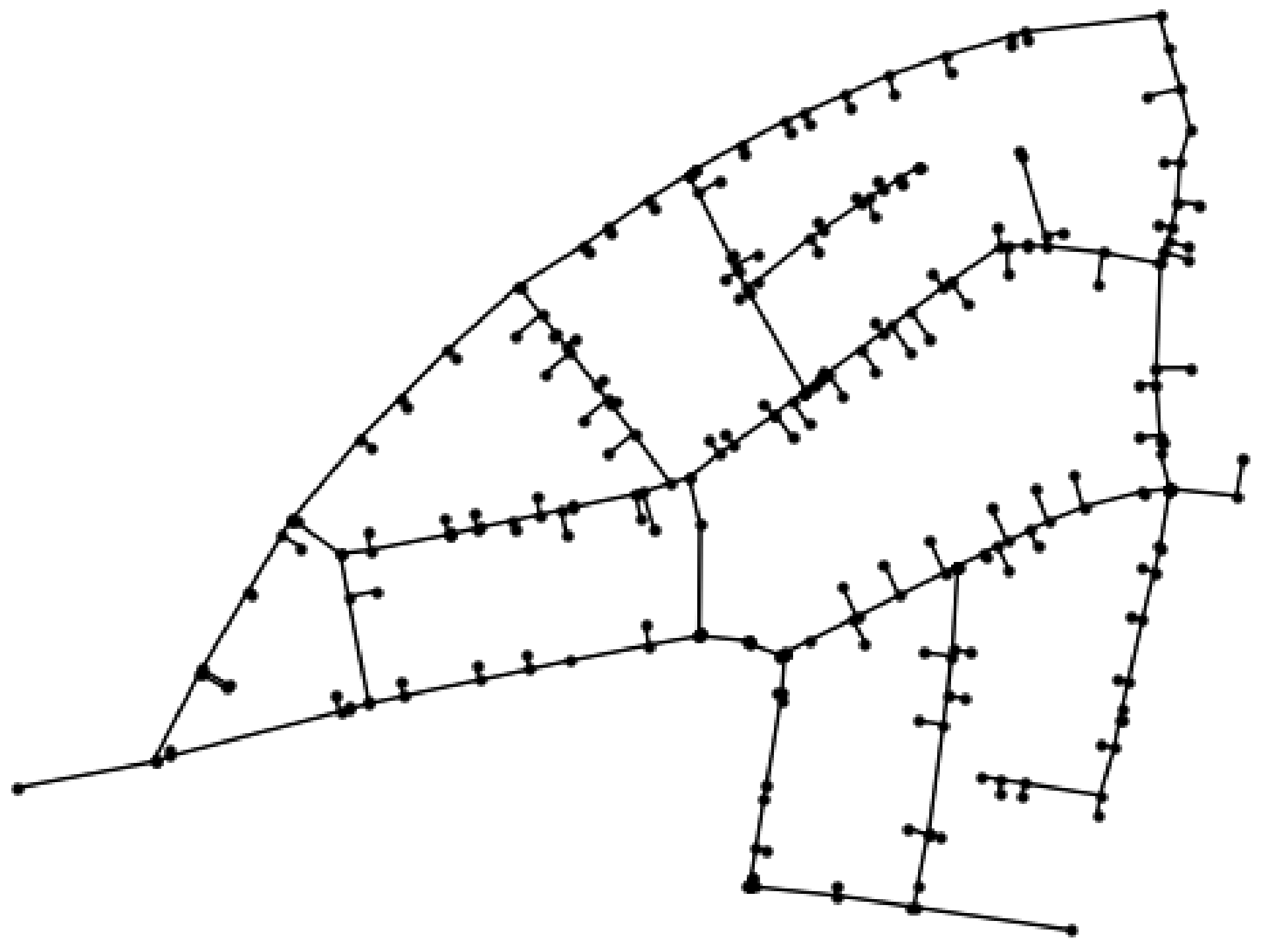
Second, a real-world water distribution network was used, namely Neptune (Figure 4), which was a pilot in the European research project Icewater [18]. Neptun is the WDN of the Romanian city of Timisoara, with an associated graph of 333 nodes (1 reservoir and 332 junctions) and 339 edges (27 valves and 312 pipes). Considering that sensors can be placed in the node, each individual of the population is a binary vector of d = 333 components.
The experiments have been run considering a budget of n s = 10 sensors. For both the two-objective formulation and four-objective formulation, 10 independent runs have been performed considering 400 generations. In the two-objective case, the objectives are the average detection time and its standard deviation, while in the four-objective case, we have also considered the average volume of contaminated water and its standard deviation. The experimental settings considered for the optimal sensor placement problem are reported in Table 2.

6.2. Results on Test Functions

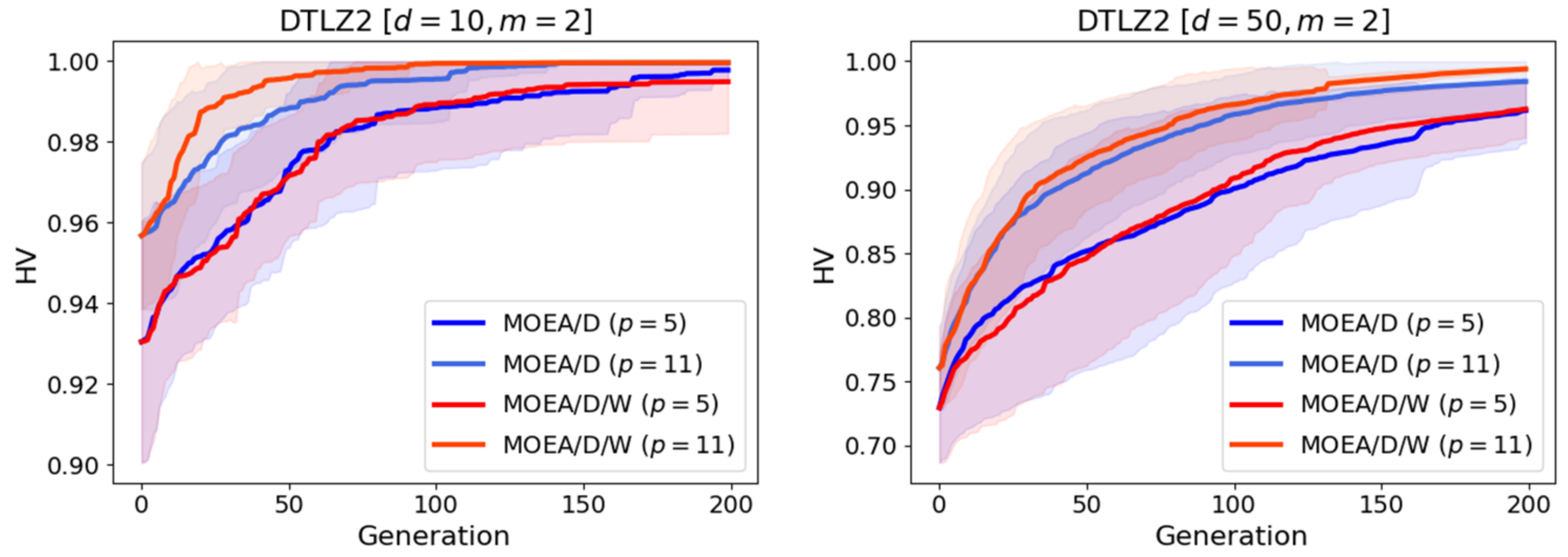
In the following figures, the results, in terms of hypervolume, on the test function DTLZ2, considering different settings, are shown.
For m = 2 MOEA/D and MOEA/D/W show the same performance in terms of hypervolume for both values of d (Figure 5).
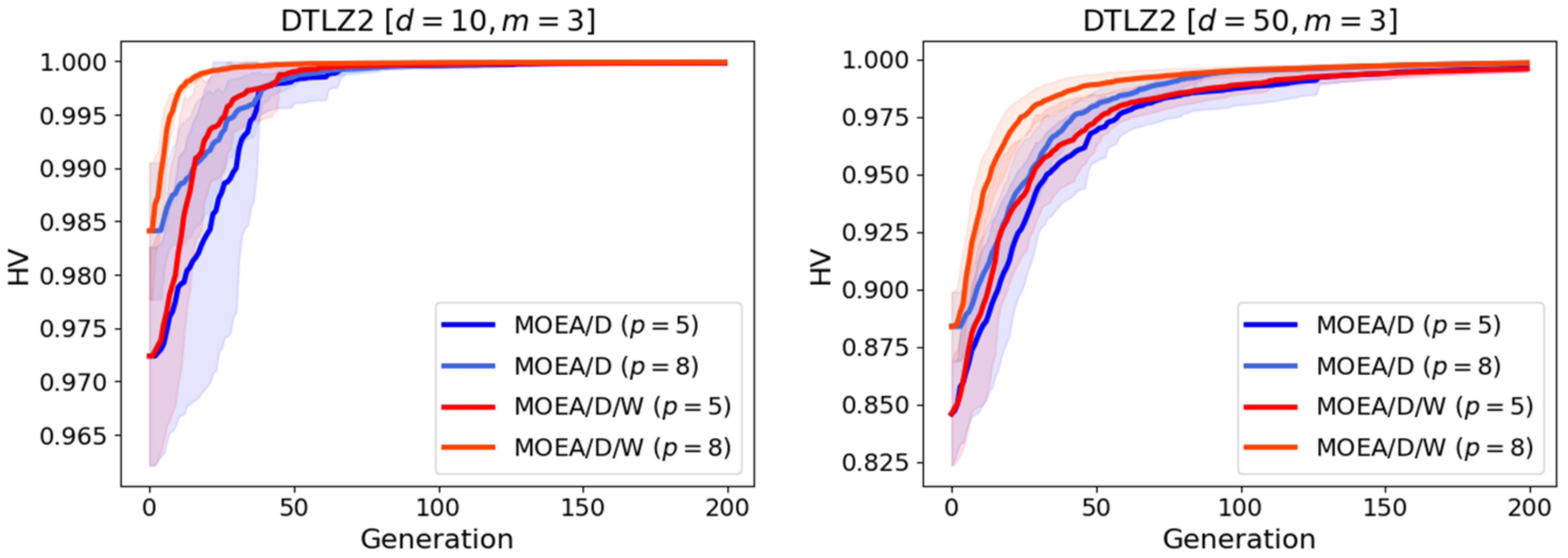
For m = 3 , MOEA/D/W is marginally better than MOEA/D for both values of d (Figure 6).
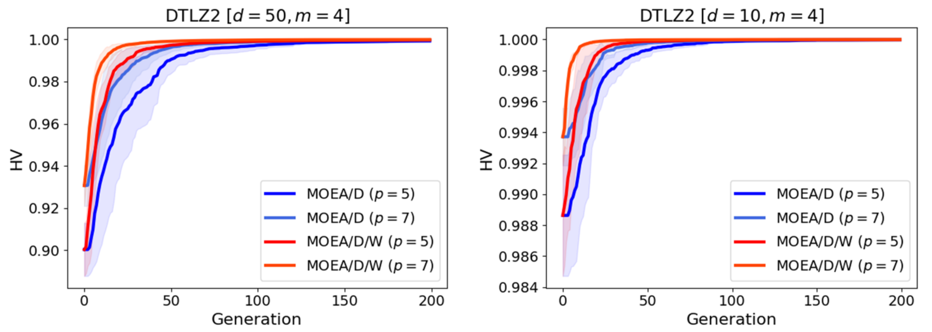
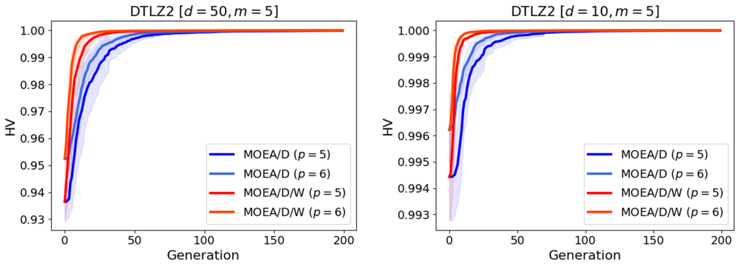
For m = 4 and m = 5 , the improvement over MOEA/D increases significantly, in particular at low generation counts (Figure 7 and Figure 8).

6.3. Results of Optimal Sensor Placement

The proposed algorithm has also been tested on the problem of optimal sensor placement on a real-world water distribution network. As shown in Figure 9, the results are coherent with the performance on the test function, reported in the previous section. In the case of m = 2 , the two algorithms are almost equivalent, while with m = 4 , the advantage of MOEA/D/W over MOEA/D increases significantly.

6.4. Discussion of the Results

Considering the test function DTLZ2, MOEA/D/W has a consistently better performance than MOEA/D: the upper bound for the value of hypervolume is reached at a lower generation count for MOEA/D/W than MOEA/D, and the improvement is more significant for a larger number of objectives. In addition, the gap in performance between the two algorithms is enhanced, increasing the number of weight vectors (i.e., the single-objective subproblems in which the multi-objective problem is decomposed), meaning that the Wasserstein distance, used in the neighbors’ selection, has better exploratory capabilities. This is highlighted in Figure 10, which shows the increase in the hypervolume of the two algorithms augmenting the population size (i.e., the number of weight vectors). The improvement in terms of performance of MOEA/D/W, doubling the population dimension, is greater than the one reported by MOEA/D, in particular at a lower generation count. Very similar behavior can be seen in the real-world problem of optimal sensor placement, in which MOEA/D/W becomes significantly better moving from two to four objectives.
Overall, in the case of DTLZ2, MOEA/D/W reaches a greater hypervolume in 78% of the experiments, while when increasing the population size, MOEA/D/W outperforms MOEA/D in 81% of the experiments. Considering the optimal sensor problem, MOEA/D/W results in a better hypervolume in 60% of the experiments, while, considering the augmented population, MOEA/D/W achieves better performance in 75% of the experiments. Needless to say, a wider set of experiments, both benchmark and real world, would be required for a full assessment of the computational performance of MOEA/D/W. The results in this section should be regarded as a “proof of concept” that using a non-Euclidean distance between combination parameters offers a promising angle in the design of a MOEA.

7. Conclusions

The key contribution of the paper is the formulation of Wasserstein-enabled selection operator of the weight parameters in the scalarization. The basic assumption is that the new operator should induce a better exploration of the space of individuals. This effect should mitigate two problems with many objectives ( m > 2 ): first, the number of incomparable solutions dominates the population, reducing the selection pressure and leading to poor convergence to the Pareto front, and second, it is more difficult to preserve diversity in the solution set. The assumption is confirmed by the experimental results of the new algorithm MOEA/D/W both for test functions and a real-world four-objective optimal sensor placement problem.
In terms of perspectives, it is fair to say that further experiments are needed to confirm the general relevance of this Wasserstein-based selection strategy. These further experiments should consider real-world problems such as disease outbreaks in networks and contact tracing in epidemics as well as a wider set of test problems.
Other approaches should also be investigated as the Gromow–Wasserstein (GW) distance for graph clustering, partitioning, and matching. Another interesting perspective is extending pressure values measured by sensors to other nodes. The Wasserstein distance can be used to propagate their measurements to the whole network, generating a distribution-valued map. This would drastically reduce the need for the simulation of the diffusion.

Author Contributions

Conceptualization, A.C. and F.A.; methodology, A.C. and A.P.; software, A.P.; validation, I.G. and A.P.; formal analysis, A.C.; investigation, A.C.; resources, I.G.; data curation, A.P.; writing—original draft preparation, A.C., F.A. and A.P.; writing—review and editing, A.C., I.G. and A.P.; visualization, A.P.; supervision, A.C. and I.G. All authors have read and agreed to the published version of the manuscript.

Funding

This study has been partially supported by the Italian project ENERGIDRICA co-financed by MIUR, ARS01_00625.

Data Availability Statement

Code and data used in this paper are available at https://github.com/andreaponti5/moeadw.

Acknowledgments

We gratefully acknowledge the DEMS Data Science Lab for supporting this work by providing computational resources (DEMS—Department of Economics, Management and Statistics).

Conflicts of Interest

The authors declare no conflict of interest.

References

  1. Cori, A.; Nouvellet, P.; Garske, T.; Bourhy, H.; Nakouné, E.; Jombart, T. A Graph-Based Evidence Synthesis Approach to Detecting Outbreak Clusters: An Application to Dog Rabies. PLoS Comput. Biol. 2018, 14, e1006554. [Google Scholar] [CrossRef]
  2. Yu, P.-D.; Tan, C.W.; Fu, H.-L. Epidemic Source Detection in Contact Tracing Networks: Epidemic Centrality in Graphs and Message-Passing Algorithms. IEEE J. Sel. Top. Signal Process. 2022, 16, 234–249. [Google Scholar] [CrossRef]
  3. Gangireddy, S.C.R.; Long, C.; Chakraborty, T. Unsupervised Fake News Detection: A Graph-Based Approach. In Proceedings of the 31st ACM Conference on Hypertext and Social Media, Online, 13–15 July 2020; pp. 75–83. [Google Scholar]
  4. Xu, W.; Wu, J.; Liu, Q.; Wu, S.; Wang, L. Evidence-Aware Fake News Detection with Graph Neural Networks. In Proceedings of the ACM Web Conference 2022, Online, 25–29 April 2022; pp. 2501–2510. [Google Scholar]
  5. Deb, K.; Pratap, A.; Agarwal, S.; Meyarivan, T. A Fast and Elitist Multiobjective Genetic Algorithm: NSGA-II. IEEE Trans. Evol. Comput. 2002, 6, 182–197. [Google Scholar] [CrossRef]
  6. Zhang, Q.; Li, H. MOEA/D: A Multiobjective Evolutionary Algorithm Based on Decomposition. IEEE Trans. Evol. Comput. 2007, 11, 712–731. [Google Scholar] [CrossRef]
  7. Monge, G. Mémoire sur la Théorie des Déblais et des Remblais. In Histoire de l’Académie Royale des Sciences de Paris; Imprimerie Royale: Louvre, France, 1781. [Google Scholar]
  8. Kantorovich, L. On the Transfer of Masses (in Russian). Proc. Dokl. Akad.Nauk. 1942, 37, 227–229. [Google Scholar]
  9. Villani, C. Optimal Transport: Old and New; Springer Science & Business Media: Berlin/Heidelberg, Germany, 2008; Volume 338. [Google Scholar]
  10. Peyré, G.; Cuturi, M. Computational Optimal Transport. arXiv 2020, arXiv:1803.00567. [Google Scholar]
  11. Redko, I.; Vayer, T.; Flamary, R.; Courty, N. CO-Optimal Transport. arXiv 2020, arXiv:2002.03731. [Google Scholar]
  12. Öcal, K.; Grima, R.; Sanguinetti, G. Parameter Estimation for Biochemical Reaction Networks Using Wasserstein Distances. J. Phys. A Math. Theor. 2019, 53, 034002. [Google Scholar] [CrossRef]
  13. Vayer, T.; Chapel, L.; Flamary, R.; Tavenard, R.; Courty, N. Optimal Transport for Structured Data with Application on Graphs. arXiv 2018, arXiv:1805.09114. [Google Scholar]
  14. Frogner, C.; Mirzazadeh, F.; Solomon, J. Learning Embeddings into Entropic Wasserstein Spaces. arXiv 2019, arXiv:1905.03329. [Google Scholar]
  15. Arjovsky, M.; Chintala, S.; Bottou, L. Wasserstein Generative Adversarial Networks. In Proceedings of the International Conference on Machine Learning, PMLR, Sydney, Australia, 6–11 August 2017; pp. 214–223. [Google Scholar]
  16. Ponti, A.; Candelieri, A.; Archetti, F. A New Evolutionary Approach to Optimal Sensor Placement in Water Distribution Networks. Water 2021, 13, 1625. [Google Scholar] [CrossRef]
  17. Margarida, D.; Antunes, C.H. Multi-Objective Optimization of Sensor Placement to Detect Contamination in Water Distribution Networks. In Proceedings of the Companion Publication of the 2015 Annual Conference on Genetic and Evolutionary Computation, Madrid, Spain, 11–15 July 2015; pp. 1423–1424. [Google Scholar]
  18. Candelieri, A.; Soldi, D.; Archetti, F. Cost-Effective Sensors Placement and Leak Localization–the Neptun Pilot of the ICeWater Project. J. Water Supply Res. Technol.—AQUA 2015, 64, 567–582. [Google Scholar] [CrossRef]
  19. Naserizade, S.S.; Nikoo, M.R.; Montaseri, H. A Risk-Based Multi-Objective Model for Optimal Placement of Sensors in Water Distribution System. J. Hydrol. 2018, 557, 147–159. [Google Scholar] [CrossRef]
  20. Beume, N.; Naujoks, B.; Emmerich, M.T.M. SMS-EMOA: Multiobjective Selection Based on Dominated Hypervolume. Eur. J. Oper. Res. 2007, 181, 1653–1669. [Google Scholar] [CrossRef]
  21. Weickgenannt, M.; Kapelan, Z.; Blokker, M.; Savic, D.A. Risk-Based Sensor Placement for Contaminant Detection in Water Distribution Systems. J. Water Resour. Plan. Manag. 2010, 136, 629–636. [Google Scholar] [CrossRef]
  22. Deb, K.; Myburgh, C. A Population-Based Fast Algorithm for a Billion-Dimensional Resource Allocation Problem with Integer Variables. Eur. J. Oper. Res. 2017, 261, 460–474. [Google Scholar] [CrossRef]
  23. Wang, Y.; van Stein, B.; Bäck, T.; Emmerich, M. A Tailored NSGA-III for Multi-Objective Flexible Job Shop Scheduling. In Proceedings of the 2020 IEEE Symposium Series on Computational Intelligence (SSCI), Canberra, Australia, 1–4 December 2020; pp. 2746–2753. [Google Scholar]
  24. Shi, J.; Sun, J.; Zhang, Q. Multi-Objectivization Inspired Metaheuristics for the Sum-of-the-Parts Combinatorial Optimization Problems. Appl. Soft Comput. 2021, 103, 107157. [Google Scholar] [CrossRef]
  25. Li, M.; Yao, X. Quality Evaluation of Solution Sets in Multiobjective Optimisation: A Survey. ACM Comput. Surv. (CSUR) 2019, 52, 1–38. [Google Scholar] [CrossRef]
  26. Knowles, J.D. ParEGO: A Hybrid Algorithm with on-Line Landscape Approximation for Expensive Multiobjective Optimization Problems. IEEE Trans. Evol. Comput. 2006, 10, 50–66. [Google Scholar] [CrossRef]
  27. Zhang, Q.; Liu, W.; Tsang, E.; Virginas, B. Expensive Multiobjective Optimization by MOEA/D with Gaussian Process Model. IEEE Trans. Evol. Comput. 2009, 14, 456–474. [Google Scholar] [CrossRef]
  28. Akimoto, Y.; Hansen, N. Projection-Based Restricted Covariance Matrix Adaptation for High Dimension. In Proceedings of the Genetic and Evolutionary Computation Conference 2016, Denver, CO, USA, 20–24 July 2016; pp. 197–204. [Google Scholar]
  29. Berry, J.; Hart, W.E.; Phillips, C.A.; Uber, J.G.; Watson, J.-P. Sensor Placement in Municipal Water Networks with Temporal Integer Programming Models. J. Water Resour. Plan. Manag. 2006, 132, 218–224. [Google Scholar] [CrossRef]
  30. Zhao, Y.; Schwartz, R.; Salomons, E.; Ostfeld, A.; Poor, H.V. New Formulation and Optimization Methods for Water Sensor Placement. Environ. Model. Softw. 2016, 76, 128–136. [Google Scholar] [CrossRef]
  31. Chowdhury, S.; Mémoli, F. The Gromov–Wasserstein Distance between Networks and Stable Network Invariants. Inf. Inference A J. IMA 2019, 8, 757–787. [Google Scholar] [CrossRef]
  32. Xu, H.; Luo, D.; Carin, L. Scalable Gromov-Wasserstein Learning for Graph Partitioning and Matching. Adv. Neural Inf. Process. Syst. 2019, 3046–3056, 1742. [Google Scholar]
  33. Xu, H. Gromov-Wasserstein Factorization Models for Graph Clustering. In Proceedings of the AAAI Conference on Artificial Intelligence, New York, NY, USA, 7–12 February 2020; Volume 34, pp. 6478–6485. [Google Scholar]
  34. Solomon, J.; Rustamov, R.M.; Guibas, L.J.; Butscher, A. Wasserstein Propagation for Semi-Supervised Learning. In Proceedings of the 31th International Conference on Machine Learning, ICML 2014, Beijing, China, 21–26 June 2014; Volume 32, pp. 306–314. [Google Scholar]
  35. Xu, H.; Luo, D.; Carin, L.; Zha, H. Learning Graphons via Structured Gromov-Wasserstein Barycenters. In Proceedings of the AAAI Conference on Artificial Intelligence, Virtual, 2–9 February 2021; Volume 35, pp. 10505–10513. [Google Scholar]
  36. Klise, K.A.; Murray, R.; Haxton, T. An Overview of the Water Network Tool for Resilience (WNTR). Available online: https://www.osti.gov/servlets/purl/1569415 (accessed on 29 March 2023).
  37. Ponti, A.; Candelieri, A.; Archetti, F. A Wasserstein Distance Based Multiobjective Evolutionary Algorithm for the Risk Aware Optimization of Sensor Placement. Intell. Syst. Appl. 2021, 10, 200047. [Google Scholar] [CrossRef]
  38. Das, I.; Dennis, J.E. Normal-Boundary Intersection: A New Method for Generating the Pareto Surface in Nonlinear Multicriteria Optimization Problems. SIAM J. Optim. 1998, 8, 631–657. [Google Scholar] [CrossRef]
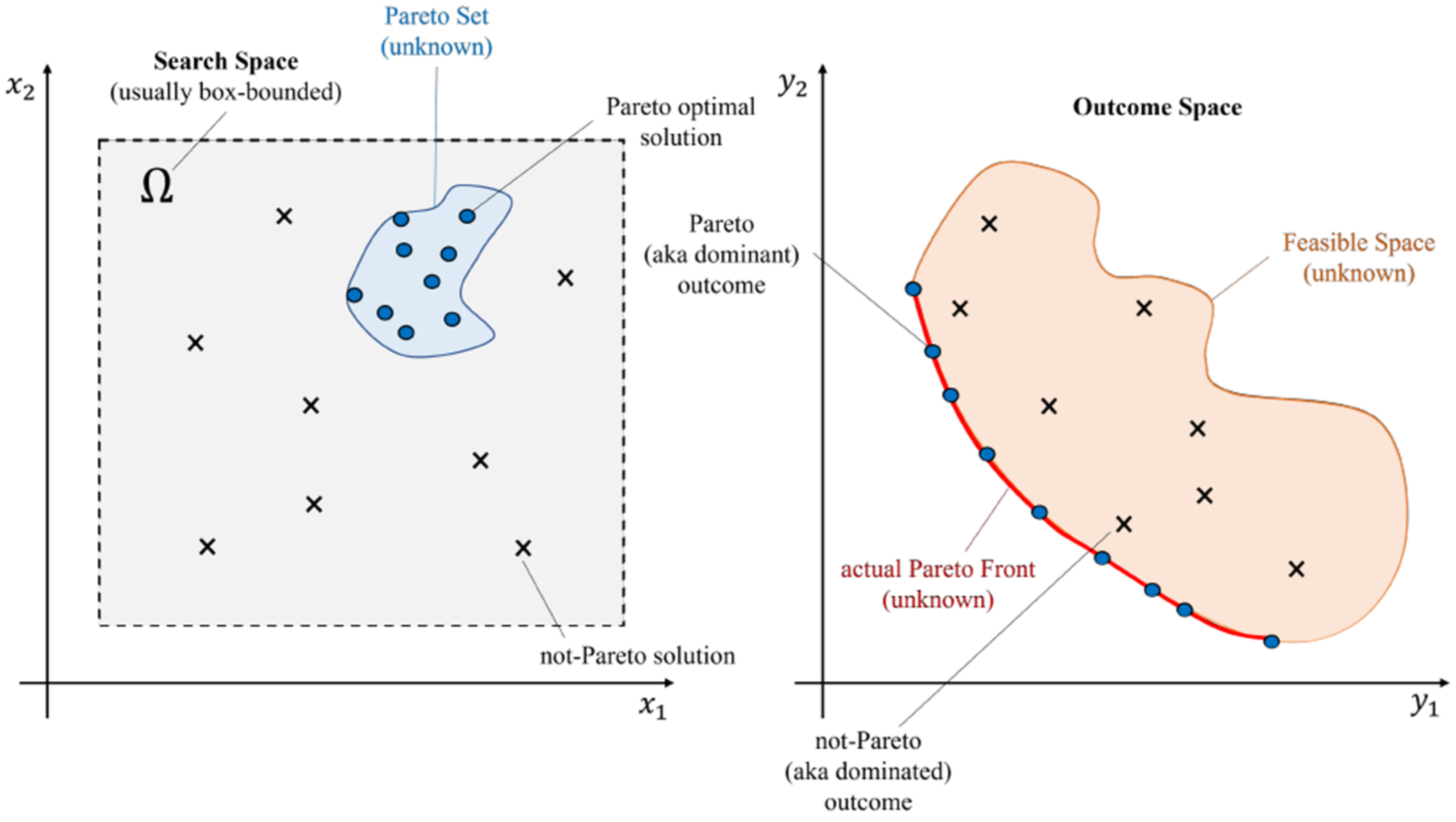
Figure 1. An example of Pareto set (left), with the associated Pareto front (right), for two minimization objectives.
Mathematics 11 02342 g001
Figure 2. Two examples of weight vectors seen as discrete probability distributions.
Mathematics 11 02342 g002
Figure 3. The Pareto front of DTLZ2 considering 2 objectives (left) and 3 objectives (right).
Mathematics 11 02342 g003
Figure 4. The water distribution network of Neptun.
Mathematics 11 02342 g004
Figure 5. Hypervolume over generations considering DTLZ2 with m = 2 and d = 10 (left) and d = 50 (right). The average hypervolume over 10 independents run is shown along with the standard deviation.
Mathematics 11 02342 g005
Figure 6. Hypervolume over generations considering DTLZ2 with m = 3 and d = 10 (left) and d = 50 (right). The average hypervolume over 10 independents run is shown along with the standard deviation.
Mathematics 11 02342 g006
Figure 7. Hypervolume over generations considering DTLZ2 with m = 4 and d = 10 (left) and d = 50 (right). The average hypervolume over 10 independents run is shown along with the standard deviation.
Mathematics 11 02342 g007
Figure 8. Hypervolume over generations considering DTLZ2 with m = 5 and d = 10 (left) and d = 50 (right). The average hypervolume over 10 independents run is shown along with the standard deviation.
Mathematics 11 02342 g008
Figure 9. Hypervolume over generations considering Neptun with m = 2 (left) and m = 4 (right). The average hypervolume over 10 independents run is shown along with the standard deviation.
Mathematics 11 02342 g009
Figure 10. The difference in hypervolume of the two algorithms increasing the population size considering both the test function (left and center) and the optimal sensor placement problem (right).
Mathematics 11 02342 g010
Table 1. Settings of the two algorithms for the test function DTLZ2.
m p N Function Evaluations
2561200
11122400
35214200
8459000
455611,200
712024,000
5512625,200
621042,000
Table 2. Settings of the two algorithms for the optimal sensor placement problem.
m p N Function Evaluations
2672800
13145600
468433,600
816566,000
Disclaimer/Publisher’s Note: The statements, opinions and data contained in all publications are solely those of the individual author(s) and contributor(s) and not of MDPI and/or the editor(s). MDPI and/or the editor(s) disclaim responsibility for any injury to people or property resulting from any ideas, methods, instructions or products referred to in the content.