A Bimodal Model for Oil Prices

Abstract

Oil price behaviour over the last 10 years has shown to be bimodal in character, displaying a strong tendency to congregate around one range of high oil prices and one range of low prices, indicating two distinct peaks in its frequency distribution. In this paper, we propose a new, single nonlinear stochastic process to model the bimodal behaviour, namely, $dp=\alpha (p_1-p)(p_2-p_{(}{p}_3-p)dt+\sigma p^{\gamma }dZ, \gamma =0,0.5$. Further, we find analytic approximations of oil price futures under this model in the cases where the stable fixed points of the corresponding deterministic model are (a) evenly spaced about the unstable fixed point and (b) are spaced in the ratio 1:2 about the unstable fixed point. The solutions are shown to produce accurate prices when compared to numerical solutions.

1. Introduction

Crude oil is one of the world’s most important commodities, not just for consumption but also as a financial asset. Futures contracts on oil are traded by financial institutions and investors for investment and risk management purposes. Successful hedging and risk management techniques, though, depend upon the accurate pricing of the contracts. In order to value financial contracts on oil, one needs to understand and develop a stochastic process that describes oil price dynamics. There are many complex factors affecting oil prices, including net demand in the market, geopolitical events, interest rates, the weather, the cost of extracting and producing oil and even market sentiment. In recent years, the corona virus pandemic saw many governments restricting travel, and businesses were forced to shut down. This led to the fall in demand for oil. In the first three months of 2020, oil consumption was down 5.6 million barrels per day to 94.4 million barrels per day. This in turn led to a drop in oil prices. In April 2020, the price for a barrel of oil fell to −USD 37.68 in the US for West Texas Intermediate (WTI) and USD 9 per barrel worldwide for Brent oil. When Russia attacked Ukraine on 24 February 2022, investors saw the potential for sanctions on Russian oil exports, which saw oil prices rocket. Large price changes over short periods are not new—they are an inherent part of the oil market. Observing the data set of oil prices over the last 10 years, it is obvious that the data are bimodal in nature (other commodities such as natural gas and food grains may also exhibit the same price pattern over this period). There is a strong tendency for prices to stay around one range of high prices and then a range of low prices before going back to the high prices and so on.

In this paper, we model the bimodal nature of oil with a nonlinear one-factor stochastic model. One-factor models are of the form $dp=A(p,t)dt+B(p,t)dZ$, where $p (=p_t)$ is the price of oil at time t, $A(p,t)$ is the drift term, $B(p,t)$ is the diffusion term, and where here and in the rest of this paper, $dZ$ is an increment in a Wiener process Z under a real probability measure. The main advantages of using one-factor models are simplicity and tractability—i.e., they can lead to closed formulae for futures prices.

An early model used to define the behaviour of commodity prices was the GBM model—i.e., Geometric Brownian Motion, in which $A(p,t)=\mu p$ and $B(p,t)=\sigma p$, where $\mu$ and $\sigma$ are constant. Using this model, Brennan and Schwartz [1] identified a relationship between spot and futures prices that included known constant convenience yields and interest rates. Using a GBM model, Gabillon [2] established a closed-form solution for futures prices of oil that depended only on the spot price of oil and a constant cost of carry of physical oil. He did, however, observe that with this formula, the term structure in backwardation could not be explained. So Gabillon extended his formula to include convenience yield. This formula could now describe both backwardation and contango states. Unfortunately, however, the formula implies a discontinuity when changing between the backwardation and contango states. Gabillon noted that use of the GBM model to value oil futures could lead to unreasonable over- or under-valuations.

Other authors suggested including mean reversion in the oil price model to capture the effect of net demand of the commodity. Using this property, Bjerksund and Ekern [3] derived the price of a European call option when the spot price follows the Ornstein–Uhlenbeck process: $A(p,t)=\eta (\mu -p), B(p,t)=\sigma$. This process can, however, generate negative prices, which, although can happen with oil prices, is very rare. In a well-known paper on futures pricing of oil, Schwartz [4] derived an analytic solution for futures prices under the mean-reverting model: $dp=\eta p(\mu -ln(p\left)\right)dt+\sigma pdZ$. Pindyck [5] also added a mean-reversion term to a deterministic linear trend model. AbaOud and Goard [6] proposed two one-factor models for oil prices with $B(p,t)=\sigma p^{\frac{3}{4}}$ and empirically showed they outperformed some well-known models in capturing the behaviour of oil prices. They also derived futures prices based on their mean-reverting models.

A number of extensions have been proposed to the one-factor model for oil prices. These include two- and three-factor models. In the two-factor models, the convenience yield and long-run mean seem to be the popular choices for the second factor. Gibson and Schwartz [7] assumed that the underlying oil price follows the GBM process and the short convenience yield follows the Ornstein–Uhlenbeck (OU) process. This was later modified by Schwartz [4], who modelled the spot price using the Geometric Ornstein–Uhlenbeck process. Some authors who considered the long-term price as a second state variable include Gabillon [2], Pilipovic [8] and Schwartz and Smith [9].

The addition of factors to the model can add complexity to the model. However, Schwartz [4] derived a futures prices under a three-factor model for oil that included the spot price, convenience yield and interest rate. In this model, the spot price follows the GBM, and the convenience yield and interest rate follow OU processes. Hilliard and Reis [10] also used the three-factor model proposed by Schwartz [2] but added jumps into the spot price process. Cortazar and Schwartz [11] proposed a three-factor model that includes spot price, convenience yield and long-term spot price return. Abadie and Chamorro [12] use mean-reverting spot price and volatility and a long-term equilibrium price that follows a GBM.

Various other modifications to the one-factor model can be found in the literature. This includes the paper by Cortazar and Naranjo [13], who used n-factor Gaussian models, and Ogbogbo [14], who considers a Levy market and uses a Levy process to model oil prices.

Examination of oil price data sets over a span of 10 years, and even just the past 5 years, shows that they are bimodal in character, showing a strong inclination to aggregate around one range of high prices and one range of low prices. No system of affine equations could lead to a finite number of non-unique fixed point solutions. Therefore, to model bimodal oil price data, we require a nonlinear model. In order to achieve this, we require only a single nonlinear equation with two stable fixed points at high and low values of oil prices, respectively. Obviously, we also need the additional external stochastic driving force, representing the unpredictable effect of many neglected influences that will enable transitions to occur between the two basins of attraction. The simplest such single-factor model is

$$dp=\alpha (p_1-p)(p_2-p)(p_3-p)dt+B(p,t)dZ,$$

(1)

with $\alpha >0$, $p_1$ the stable low fixed point, $p_3$ the stable high fixed point and $p_2$ an unstable intermediate fixed point. In the neighbourhood of $p=p_1$, oil prices revert to $p_1$ as

$$p=p_1{e}^{-\alpha (p_2-p_1)(p_3-p_1)t}$$

(2)

with time scale $1/\left[\alpha (p_2-p_1)(p_3-p_1)\right]$. Similarly, in the neighbourhood of $p=p_3$, oil prices revert to $p_3$ exponentially with a time scale $1/\left[\alpha (p_3-p_2)(p_3-p_1)\right]$.

For an initial value $p_0$ strictly between $p_1$ and $p_2$, the full solution to the nonlinear deterministic model (i.e., (1) with $B(p,t)=0$) is

$$t=-\frac{1}{\alpha }ln\left({\left[\frac{p-p_1}{p_0-p_1}\right]}^{a_1}{\left[\frac{p-p_3}{p_0-p_3}\right]}^{a_3}{\left[\frac{p-p_2}{p_0-p_2}\right]}^{-a_2}\right),$$

where

$$\begin{array}{ccc}\hfill a_1& =& \frac{p_3-p_2}{(p_2-p_1)p_3^2-(p_3-p_1)p_2^2+(p_3-p_2)p_1^2},\hfill \\ \hfill a_2& =& \frac{p_1-p_3}{(p_2-p_1)p_3^2-(p_3-p_1)p_2^2+(p_3-p_2)p_1^2},\hfill \\ \hfill a_3& =& \frac{p_2-p_1}{(p_2-p_1)p_3^2-(p_3-p_1)p_2^2+(p_3-p_2)p_1^2}.\hfill \end{array}$$

Similar solutions can be found for other initial conditions simply by separation of variables and integration by partial fractions.

The occasional switching between the zone of low oil price, with interval of attraction $[0,p_2)$, and the zone of high oil price, with interval of attraction $(p_2,\infty )$, occurs because of the random excursion $B(p,t)dZ$. This simple device for modelling bimodal oil price dynamics is to be compared with the device of deterministic chaos, which requires at least three coupled autonomous differential equations, two coupled non-autonomous equations or two coupled difference equations.

The goal of this paper is two-fold:

• To model oil prices, we want to demonstrate the significance of the cubic term in Equation (1) with $B(P,t)=\sigma p^{\gamma }$ (which we call our unrestricted model). To do this, in Section 2, we compare the ability to capture oil price behaviour of several existing one-factor stochastic models for oil prices that are subsets of the unrestricted model. The estimation technique that we use to compare these models is the statistical method of the Generalized Method of Moments (GMM). This method combines the observed data with the information in population moment conditions to generate estimates of the unknown parameters in the given model. Using 10 years of data, we empirically test the nested models and explain the results.
• Having justified the need for a cubic drift term, in Section 3, we formulate analytic approximate solutions to futures prices under (1) with $B(p,t)=\sigma$ and $B(p,t)=\sigma p^{\frac{1}{2}}$.

We present our conclusion in Section 4.

2. Motivation for the Bimodal Model—An Empirical Study

In this section, we empirically test ten oil price models that are nested within our unrestricted model for their ability to capture the dynamics of oil price movements. The estimation technique that we use to compare these models is the Generalized Method of Moments (GMM), which is a method used to find efficient estimates of parameters when the number of moment conditions is larger than the number of parameters being estimated. The method is summarised in Appendix A, but for a more detailed explanation, the reader is referred to Hayashi [15], Mackinlay and Richardson [16] and also Ferson and Foerster [17].

2.1. The Models to Be Tested

Table 1. Models to be tested in the form $dp=A(p,t)dt+B(p,t)dZ$.

Model	$\mathit{A}(\mathit{p},\mathit{t})$	$\mathit{B}(\mathit{p},\mathit{t})$
1	$(k_1+k_{2}p+k_3{p}^2+k_4{p}^3)$	$\sigma p^{1/2}$
2	$(k_1+k_{2}p)$	$\sigma p^{1/2}$
3	$(k_{2}p+k_3{p}^2)$	$\sigma p^{1/2}$
4	$k_{2}p$	$\sigma p$
5	$k_{2}p$	$\sigma p^{1/2}$
6	$(k_1+k_{2}p+k_3{p}^2+k_4{p}^3)$	$\sigma$
7	$(k_1+k_{2}p)$	$\sigma$
8	$(k_{2}p+k_3{p}^2)$	$\sigma$
9	$k_{2}p$	$\sigma$
10	$(k_{2}p+k_3{p}^2)$	$\sigma p^{3/2}$

lists the ten stochastic models of the form $dp=A(p,t)dt+B(p,t)dZ$ that were examined for their capability of fitting oil prices. They can each be nested within the unrestricted model

$$dp=(k_1+k_{2}p+k_3{p}^2+k_4{p}^3)dt+\sigma p^{\gamma }dZ,$$

(3)

where $k_1,k_2,k_3,k_4,M$ and $\gamma$ are constants, by placing restrictions on certain parameters as given in

Table 2. Parameter restrictions on unrestricted models (3).

Model	${\mathit{k}}_1$	${\mathit{k}}_2$	${\mathit{k}}_3$	${\mathit{k}}_4$	$\mathit{\gamma }$
1					0.5
2			0	0	0.5
3	0			0	0.5
4	0		0	0	1
5	0		0	0	0.5
6					0
7			0	0	0
8	0			0	0
9	0		0	0	0
10	0			0	1.5

.

In Models 1–3 and 5, the diffusion term follows the square-root process, which is the type used by Heston [18] to model volatility. This implies that the volatility of the percentage change in price is a decreasing function of p. The diffusion term in Models 6–9 means that the volatility of p is constant in absolute terms.

Model 4 is the Geometric Brownian Motion used by Black and Scholes [19] to value European options. It infers an instantaneous growth rate of $k_2$ and presumes that the volatility of percentage changes and the expected percentage change in prices are constant. It was also used to value oil by Brennan and Schwarz [1], McDonald and Siegel [20] and Gabillon [2].

The drift term in Models 2 and 7 can be written as $-k_2(\frac{-k_1}{k_2}-p)$. With $k_1>0,k_2<0,$ the models are mean-reverting in nature, where the price reverts to the constant $\frac{-k_1}{k_2}$ with reversion rate $-k_2$. Larger values of $|k_2|$ mean faster reversion to the long-run mean $\frac{-k_1}{k_2}$. These models are then referred to as the Heston model and the Mean-Reverting Gaussian, respectively.

In Models 3, 8 and 10, we can write the nonlinear drift term as $-k_{3}p(\frac{-k_2}{k_3}-p)$. If $k_2>0,k_3<0$, then these models are also mean-reverting in nature, where the price reverts to the constant $\frac{-k_2}{k_3}$ with a reversion rate that depends on p. Model 10 was used by Goard to model interest rates [21] and volatility [22,23]. The $3/2$ power in the diffusion term proved useful to reduce the heteroskedasticity (heteroskedasticity means that the variance of the errors varies widely across the observations) of interest rates and volatility.

2.2. The Data

For our GMM analysis, Brent crude oil spot prices (sampled both weekly and monthly) between January 2013 and December 2022 were collected from the U.S. Energy Information Administration. The prices are plotted in Figure 1. From this figure, it can be seen that in the period 2013–2016 (from 0 to 37 in (a) and 0 to 159 in (c)) prices decreased and reached about USD 28 per barrel. In this time, the demand for oil was low, but at the same time there was overproduction of oil. As a result, the Organization of the Petroleum Exporting Countries (OPEC) aimed to support oil prices by agreeing to reduce crude supply. This decision can be considered to be the most important factor that caused the increase in oil prices over the period 2016–2020 (from 38–86 in (a) and from 160–374 in (c)). However, the global pandemic (COVID-19) had a detrimental impact on the oil market as most countries enforced strict social distancing and lockdowns to control virus expansion. This caused a dive in oil demand and a historical low spot price was recorded (below USD 20 per barrel). Since then (from mid 2020 to 2022), oil prices have seen an increasing trend due to many factors, but most importantly, OPEC’s reduction of crude supply and the Russian invasion of Ukraine in February 2022.

Table 3. Standard statistics for Brent crude oil (weekly and monthly) spot prices 2013–2022.

Standard Statistics	Weekly Data	Monthly Data
Mean	70.61	70.64
Median	64.82	64.56
Standard Deviation	24.95	24.87
Sample Variance	622.44	618.30
Kurtosis	−0.86	−0.88
Skewness	0.40	0.41
Range	113.16	104.33
Minimum	14.24	18.38
Maximum	127.40	122.71
number of observation	520	120

shows the standard statistics for Brent crude oil (weekly and monthly) spot prices 2013–2022. We see that the mean price in our period of study is about USD 70 and the standard deviation is about USD 25. The minimum and maximum are very close to the same distance from the mean, while the mean is close to the median. Both of these observations are consistent with low skewness. Further, both the minimum and maximum are just over two standard deviations from the mean, which is consistent with slightly negative kurtosis.

From Figure 1, we can see the bimodal nature of the data with the stable low fixed point in the interval [44, 50] and the stable high point in the interval [104, 110]. The histograms confirm the bimodality of the data.

2.3. Performance of Nested Models

We now compare Models 1–10, which are listed in Table 1, for their ability to capture the behaviour of Brent crude oil prices in the 10 years between 2012 and 2022. As mentioned in Section 2.1, each model can be nested within the unrestricted model (3), which we use as a benchmark to compare the performances of each of the nested models.

In particular, GMM was used to estimate the parameters of the continuous-time model for $\eta =\frac{p}{100}$, whereby Itô’s Lemma, $\eta$ follows

$$d\eta =(c_1+c_2\eta +c_3{\eta }^2+c_4{\eta }^3)dt+M{\eta }^{\gamma }dZ$$

(4)

where

$$\begin{array}{ccc}\hfill c_1& =& k_1/100,\hfill \\ \hfill c_2& =& k_2,\hfill \\ \hfill c_3& =& 100k_3,\hfill \\ \hfill c_4& =& {100}^2{k}_4,\hfill \\ \hfill M& =& \sigma {100}^{\gamma -1}.\hfill \end{array}$$

Table A1. Empirical Results for Nesting Models 1–10 within (3) using 10 years of monthly data.

Model	${\mathit{c}}_1$	${\mathit{c}}_2$	${\mathit{c}}_3$	${\mathit{c}}_4$	M	$\mathit{\gamma }$	${\mathit{\chi }}^2$ p-Value	DF
Unrestricted	3.221	−14.544	20.796	−9.382	−0.2329	0.1277	N/A	N/A
	[0.001]	[0.002]	[0.005]	[0.008]	[<0.001]	[0.520]
1	3.448	−14.818	20.628	−9.170	−0.2426	0.5	0.09	1
	[<0.001]	[0.002]	[0.005]	[0.009]	[<0.001]
2	0.502	−0.6844	0	0	0.2415	0.5	0.005	3
	[0.009]	[0.011]			[<0.001]
3	0	0.6214	−0.7370	0	0.2404	0.5	0.001	3
		[0.040]	[0.027]		[<0.001]
4	0	0.3878	0	0	−0.500	1	0	4
		[0.329]			[<0.001]
5	0	0.111	0	0	−0.5302	0.5	0	4
		[0.779]			[<0.001]
6	3.086	−14.275	20.711	−9.427	0.2242	0	0.514	1
	[0.002]	[0.004]	[0.006]	[0.009]	[<0.001]
7	0.2878	−0.4651	0	0	0.2262	0	0.030	3
	[0.165]	[0.102]			[<0.001]
8	0	0.2641	−0.4071	0	0.2291	0	0.016	3
		[0.394]	[0.230]		[<0.001]
9	0	−0.096	0	0	0.2392	0	0.017	4
		[0.289]			[<0.001]
10	0	0.9125	−1.006	0	0.2023	1.5	0	3
		[0.001]	[0.001]		[<0.001]

and

Table A2. Empirical Results for Nesting Models 1–10 within (3) using 10 years of weekly data.

Model	${\mathit{c}}_1$	${\mathit{c}}_2$	${\mathit{c}}_3$	${\mathit{c}}_4$	M	$\mathit{\gamma }$	${\mathit{\chi }}^2$ p-Value	DF
Unrestricted	2.696	−12.825	19.137	−8.895	0.2284	0.3140	N/A	N/A
	[0.091]	[0.074]	[0.063]	[0.056]	[<0.001]	[0.064]
1	2.9398	−13.897	20.774	−9.682	0.2390	0.5	0.282	1
	[0.061]	[0.049]	[0.040]	[0.034]	[<0.001]
2	0.1993	−0.255	0	0	−0.234	0.5	0.122	3
	[0.272]	[0.316]			[<0.001]
3	0	0.3238	−0.3769	0	−0.2346	0.5	0.125	3
		[0.255]	[0.252]		[<0.001]
4	0	0.0717	0	0	−0.2464	1	0	4
		[0.378]			[<0.001]
5	0	0.014	0	0	−0.2389	>0.5	0.134	4
		[0.864]			[<0.001]
6	2.167	−10.343	15.316	−7.081	0.201	0	0.065	1
	[0.175]	[0.150]	[0.135]	[0.125]	[<0.001]
7	0.0987	−0.1804	0	0	−0.1990	0	0.116	3
	[0.593]	[0.483]			[<0.001]
8	0	0.1199	−0.2020	0	−0.1991	0	0.121	3
		[0.681]	[0.547]		[<0.001]
9	0	−0.052	0	0	−0.2014	0	0.185	4
		[0.526]			[<0.001]
10	0	0.7269	−0.7831	0	−0.2290	1.5	0	3
		[0.009]	[0.015]		[<0.001]

in Appendix B present the results from the GMM analysis using 10 years of monthly and 10 years of weekly data, respectively. In the tables, ‘DF’ stands for degrees of freedom.

Table A1 presents the results from the 10 years of monthly data. The tables provide very strong evidence of the importance of the cubic drift term when explaining variation in oil prices. Every coefficient in the cubic drift term is statistically significantly different from zero at the $1\%$ level of significance. The ${\chi }^2$ p-values indicate that only Models 1 and 6, which include all the cubic terms, are acceptable at the $5\%$ level of significance, with Model 6 (which has $\gamma =0$) not being able to be rejected even at the 50% level of significance. All the other models are rejected or misspecified in terms of their overidentifying restrictions. In other words, the restrictions on these models are unreasonable.

Table A2 has the results from the 10 years of weekly data. Every coefficient in the cubic drift term is statistically significantly different from zero at the $10\%$ level of significance. However, it is clear that the value of $\gamma$ is also an important parameter differentiating the models. The ${\chi }^2$ p-values of models with $\gamma =1,1.5$ (Models 4 and 10) indicate that these models are rejected at the 1% level of significance. It is interesting that in Models 2, 3, 5, 7, 8 and 9, the coefficients in the drift term are individually not statistically significantly different from zero, but jointly they are statistically significantly different from zero. Model 1, with all nonzero coefficients in the cubic drift term and with $\gamma =0.5$, has the highest p-values of the overidentification tests and cannot be rejected even at the 25% level of significance.

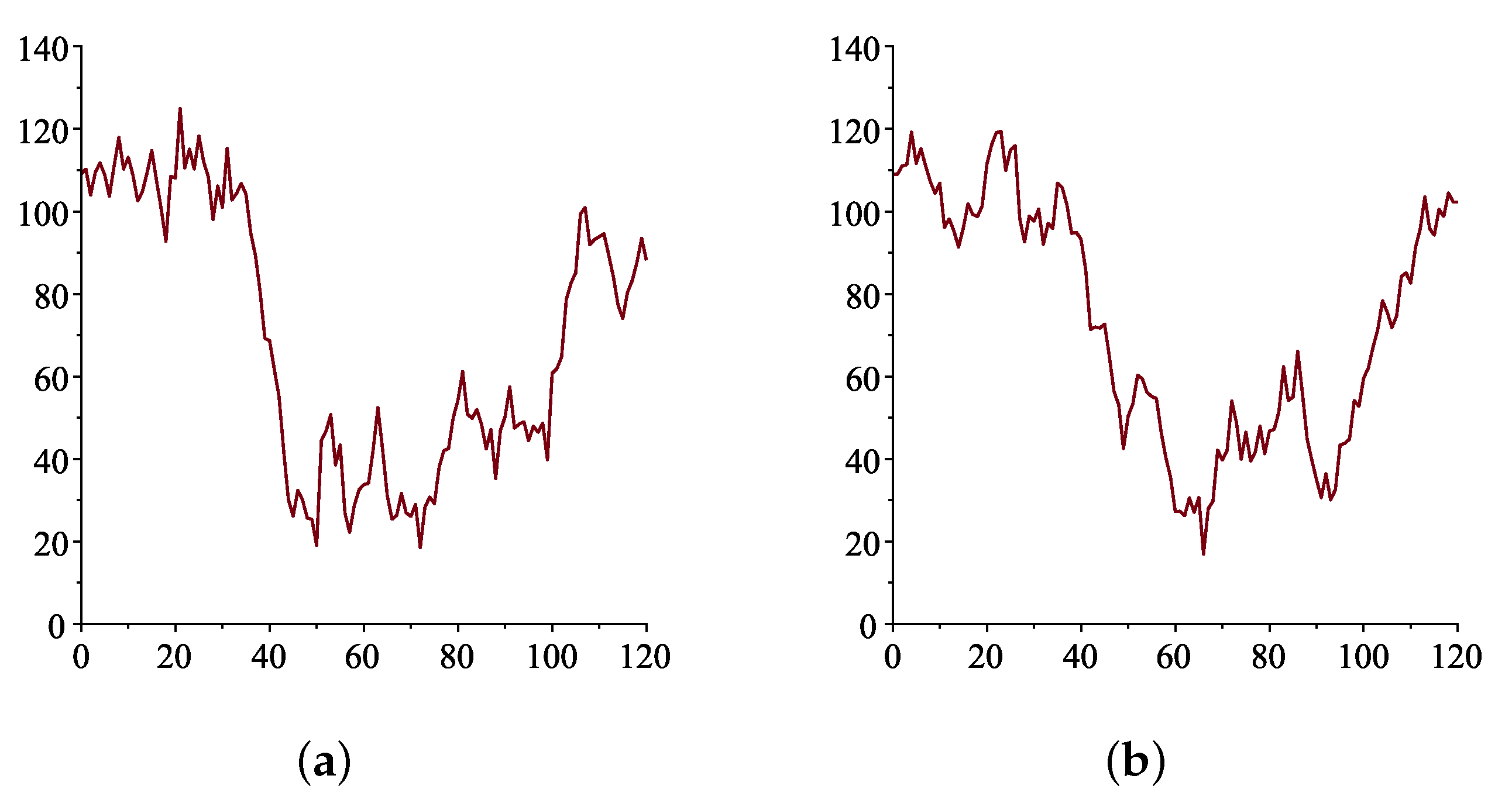
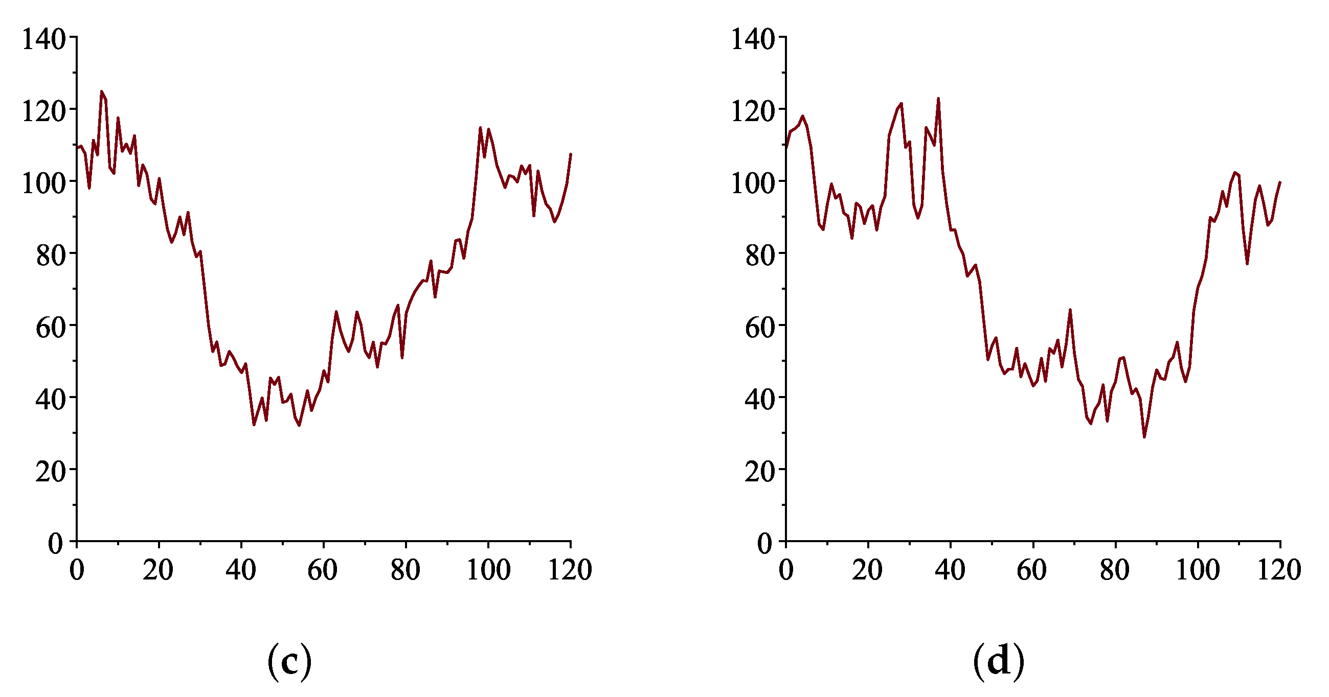
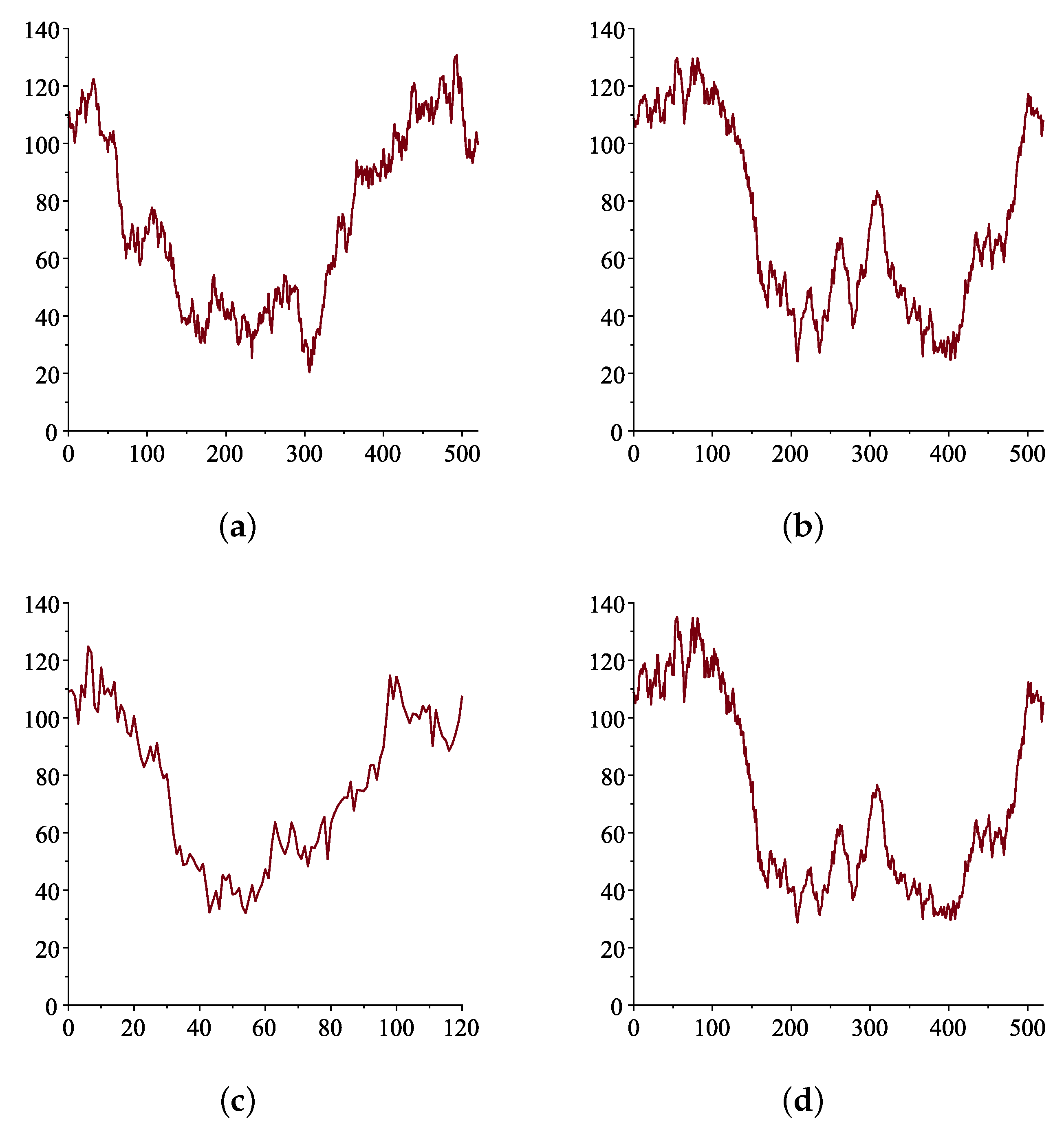
We note that we also did a similar analysis with the 5 years of data from 2017 and 2022 and found very similar results. As a further note, from the GMM results, the data infer that the $p_i$ values are generally such that $|p_3-p_2|=2|p_2-p_1|$. However, when $\gamma =0$, we could also use the approximation $|p_3-p_2|=|p_2-p_1|$. We simulated the oil price data over 10 years, both monthly and weekly, with the parameter values provided by the GMM results. See Figure A1 and Figure A2, where in Figure A1 we have monthly simulations and in Figure A2 we have weekly simulations. Comparing these with the plots of the true data in Figure 1, we see that they can mimic the essential features of the true oil price movement. For example, they have values congregating around $p_1$ and $p_3$, and the prices switch between these two regions. The range of values are also the same, staying in the interval [18, 125]. Note that in Figure A1a,c we have $|p_1-p_2|=|p_2-p_3|$ with $\gamma =0$ and 1.5, respectively, and in Figure A1b,d we have $|p_1-p_2|=2|p_2-p_3|$ with $\gamma =0$ and 1.5, respectively. Similarly, in Figure A2a,c we have $|p_1-p_2|=|p_2-p_3|$ with $\gamma =0$ and 1.5, respectively, and in Figure A2b,d we have $|p_1-p_2|=2|p_2-p_3|$ with $\gamma =0$ and 1.5, respectively.

3. Analytic Futures Prices under Model (3)

Given that the real process for $p(=p_t)$ is of the form

$$dp=\alpha (p_1-p)(p_2-p)(p_3-p)dt+\sigma p^{\gamma }dZ,$$

(5)

then allowing for the possibility of a nonzero market price of risk, $\lambda (p,t)$, associated with oil prices, the risk-neutral process will be

$$dp=[\alpha (p_1-p)(p_2-p)(p_3-p)-\lambda (p,t)\sigma p^{\gamma }]dt+\sigma p^{\gamma }d\overline{Z},$$

(6)

where $\overline{Z}$ is a Wiener process under an equivalent risk-neutral probability measure under which p becomes a martingale. One way $\lambda (p,t)$ can be found is by implying it from market futures prices, i.e., choosing a ${\lambda }^{*}$ that minimises the error between market and model prices. This usually involves assuming a form for the market price of risk (see, e.g., Egloff et al. [24]). Here, like many other authors (e.g., Stein and Stein [25] and Grünbichler and Longstaff [26]), we assume that the market price of risk $\lambda (p,t)$ is such that the forms of the real and risk-neutral processes are alike. This means that when $\gamma =0$, then $\lambda (p,t)=d_0+d_{1}p+d_2{p}^2+d_3{p}^3$, and when $\gamma =0.5$, then $\lambda (p,t)=f_0{p}^{-0.5}+f_1{p}^{0.5}+f_2{p}^{3/2}+f_3{p}^{5/2}$, where $d_i,f_i,i=0,1,2,3$ are constants. Without loss of generality, for convenience we will still use the same notation for the constants.

The partial differential equation (PDE) that governs futures prices under the risk-neutral process

$$dp=\alpha (p_1-p)(p_2-p)(p_3-p)dt+\sigma p^{\gamma }d\overline{Z},$$

(7)

is given by (see [27])

$$F_{\tau }=\frac{{\sigma }^2{p}^{2\gamma }}{2}{F}_{pp}+\alpha (p_1-p)(p_2-p)(p_3-p)F_p,$$

(8)

where $F(p,0)=p$. From the GMM analysis of Section 2.3, we choose to consider only the cases $\gamma =0$ and $\gamma =1/2$. We start by non-dimensionalising the problem. This ensures that the relative sizes of different variables are obvious and signifies the important variables and constants in the equation. Hence, we let $z=\frac{F}{p_1}, y=\frac{p}{p_1}$ and ${\tau }_b=\tau \alpha p_1^2$. This reduces the problem to

$$z_{{\tau }_b}=ϵy^{2\gamma }{z}_{yy}+(1-y)(q_2-y)(q_3-y)z_y, \mathrm{where} ϵ=\frac{{\sigma }^2{p}_1^{2\gamma -4}}{2\alpha },$$

(9)

and $q_2=\frac{p_2}{p_1}$, $q_3=\frac{p_3}{p_1},$ to be solved subject to $z(y,0)=y$. Hence, once $z(y,{\tau }_b)$ is calculated, we then have $F=p_{1}z\left(\frac{p}{p_1},\tau \alpha p_1^2\right).$ However, to the best of the authors’ knowledge, PDE (9) has no analytic solution, and so we look for a good analytic approximation.

Given that $p_1$ is large and we are considering $\gamma =0,0.5$, then $ϵ$ is assumed small $(\ll 1)$. Hence, we seek a perturbation solution of the form

$$z=z_0+ϵz_1+{ϵ}^2{z}_2+\dots$$

(10)

where $z_0(y,0)=y, z_i(y,0)=0$ for $i=1,2,3\dots$. Substituting (10) into (9) and collecting the coefficients of ${ϵ}^0$, we get that $z_0$ needs to satisfy

$${\left(z_0\right)}_{{\tau }_b}=(1-y)(q_2-y)(q_3-y){\left(z_0\right)}_y$$

(11)

subject to $z_0(y,0)=y$. Note, this equation is independent of $\gamma$.

Solving (11) by the method of characteristics gives

$$z_0=\overline{\varphi }\left[\frac{e^{-{\tau }_b}{(1-y)}^{\frac{1}{(q_2-1)(q_3-1)}}{(q_3-y)}^{\frac{1}{(q_3-1)(q_3-q_2)}}}{{(q_2-y)}^{\frac{1}{(q_2-1)(q_3-q_2)}}}\right],$$

(12)

where we need $z_0=y$ when ${\tau }_b=0$. This is hard to solve for the function $\overline{\varphi }$ for arbitrary $q_1,q_2,q_3$. However, we recall from the GMM analysis that if we let $q_2=1+{ϵ}_2, q_3=1+{ϵ}_2+{ϵ}_3$, then we can well approximate ${ϵ}_3$ by ${ϵ}_2$ or $2{ϵ}_2$. Hence, we will study these two cases and will get solutions for futures prices of the form

$$F=p_{1}z\left(\frac{p}{p_1},\tau \alpha p_1^2\right)$$

where $z=z_0+ϵz_1$ with

1. ${ϵ}_3={ϵ}_2$ when (a) $\gamma =0$ and (b) $\gamma =0.5$ and

2. ${ϵ}_3=2{ϵ}_2$ when (a) $\gamma =0$ and (b) $\gamma =0.5.$

As explained further in the paper, if higher-order approximations $z_2,z_3,\dots$ are needed, then they can be found in a similar way to $z_1$.

3.1. Case ${ϵ}_3={ϵ}_2$

Here we assume ${ϵ}_3={ϵ}_2$, so we have $q_2=1+{ϵ}_2$ and $q_3=1+2{ϵ}_2$. We now approximate z under this assumption by finding $z_0$ and $z_1$ as in (10).

3.1.1. The O(1) Term $z_0$

With ${ϵ}_3={ϵ}_2$, without loss of generality, from (12) we may write

$$\begin{array}{cc}\hfill z_0& =\varphi \left[\frac{e^{-2{ϵ}_2^2{\tau }_b}(1-y)(q_3-y)}{{(q_2-y)}^2}\right],\hfill \end{array}$$

for some function $\varphi$ so that $z_0(y,0)=y$.

By letting $Y=1-y$ at ${\tau }_b=0$, we need to find $\varphi$ so that

$$\begin{array}{cc}\hfill 1-Y& =\varphi \left[\frac{Y(Y+2{ϵ}_2)}{{(Y+{ϵ}_2)}^2}\right].\hfill \end{array}$$

We let

$$\overline{\xi }=\frac{Y(Y+2{ϵ}_2)}{{(Y+{ϵ}_2)}^2}$$

(13)

and solve for Y (and hence y) in terms of $\overline{\xi }$. This gives us

$$Y=-{ϵ}_2\pm {ϵ}_2\frac{\sqrt{1-\overline{\xi }}}{1-\overline{\xi }}.$$

(14)

Hence, $\varphi \left(\overline{\xi }\right)=1+{ϵ}_2\left(1\mp \frac{1}{\sqrt{1-\overline{\xi }}}\right)$. However, to satisfy the initial condition, we must use the positive sign when $y>q_2$, and when $y<q_2$ we must use the negative sign. This then leads to the solution for all y:

$$z_0=1+{ϵ}_2\left(1+\frac{y-q_2}{\sqrt{{(q_2-y)}^2-e^R(1-y)(q_3-y)}}\right), \mathrm{where} R=-2{ϵ}_2^2{\tau }_b.$$

(15)

[Note that in terms of the original variables we get $F=p_{1}z\left(\frac{p}{p_1},\tau \alpha p_1^2\right)$, and, hence,

$$\begin{array}{c}\hfill F(p,\tau )=p_2+\frac{(p_2-p_1)(p-p_2)}{\sqrt{{(p_2-p)}^2-e^{\overline{R}}(p_1-p)(p_3-p)}}, \mathrm{where} \overline{R}=-2\tau \alpha {ϵ}_2^2{p}_1^2.\end{array}$$

We also note that we can simplify $p_2-p_1=p_1{ϵ}_2$.]

Figure 2 illustrates the solution $z_0$, in which $q_2$ and $q_3$ are approximately 1.52 and 2.04, respectively. We see that when $y<1$, the solution increases with ${\tau }_b$ (contango). When $1<y<q_2$, the solution decreases with ${\tau }_b$ (backwardation), and then, when $q_2<y<q_3$, the solution again increases with ${\tau }_b$. This is to be expected, as $p_1$ and $p_3$ are the stable fixed points.

3.1.2. The $O\left(ϵ\right)$ Term $z_1$

We now consider two cases for the approximation $z_1$: when $\gamma$ = 0, so $ϵ=\frac{{\sigma }^2}{2\alpha p_1^4}$, and when $\gamma =0.5$, so $ϵ=\frac{{\sigma }^2}{2\alpha p_1^3}$, in (9).

Subcase $\mathbf{\gamma }=\mathbf{0}$ in (9)

Substituting (10) into (9) and collecting the coefficients of ${ϵ}^1$, we get that with $\gamma =0$, $z_1$ needs to satisfy

$${\left(z_1\right)}_{{\tau }_b}={\left(z_0\right)}_{yy}+(1-y)(q_2-y)(q_3-y){\left(z_1\right)}_y$$

(16)

subject to $z_1(y,0)=0.$ Solving (16) by the method of characteristics (see [28]), we get $z_1=\psi \left(\xi \right)-Q$, where ${\displaystyle \xi =e^{-2{ϵ}_2^2{\tau }_b}\frac{(1-y)(q_3-y)}{{(q_2-y)}^2}}$, and ${\displaystyle Q=\int \frac{f\left(y\right)}{(1-y)(q_2-y)(q_3-y)}dy,}$ where $f\left(y\right)={\left(z_0\right)}_{yy}$ with $e^{-2{ϵ}_2^2{\tau }_b}$ replaced by ${\displaystyle \frac{A{(1+{ϵ}_2-y)}^2}{(1-y)(1+2{ϵ}_2-y)}}$ with A constant.

After integration, we then replace A with ${\displaystyle \frac{e^{-2{ϵ}_2^2{\tau }_b}(1-y)(1+2{ϵ}_2-y)}{{(1+{ϵ}_2-y)}^2}.}$

This gives

$$\begin{array}{ccc}\hfill Q& =& \frac{X(q_2-y)}{{ϵ}_2{[{(q_2-y)}^2-X(1-y)(q_3-y)]}^{\frac{5}{2}}}\ast \hfill \\ & & \left\{-\frac{3X}{16}({(1-y)}^2+{(q_3-y)}^2)+\frac{3}{2}(1-y)(q_3-y)\right.\hfill \\ & & +\frac{15X}{8}(1-y)(q_3-y)+\frac{3}{2}{(q_2-y)}^2\hfill \\ & & +\frac{3}{{ϵ}_2^2}(1-y)(q_3-y){(q_2-y)}^{2}ln\left(\frac{(1-y)(q_3-y)}{{(q_2-y)}^2}\right)\hfill \\ & & \left.+\frac{3X}{2{ϵ}_2^2}{(1-y)}^2{(q_3-y)}^{2}ln\left(\frac{(1-y)(q_3-y)}{{(q_2-y)}^2}\right)\right\},\hfill \end{array}$$

(17)

where $X=exp(-2{ϵ}_2^2{\tau }_b)$. To find $\psi \left(\xi \right)$, we use the initial condition at $\tau =0$ that $z_1=0$, so we need

$$\begin{array}{c}\hfill \psi \left(\overline{\xi }\right)=Q\left(\overline{\xi }\right) \mathrm{where} \overline{\xi }=\frac{(1-y)(q_3-y)}{{(q_2-y)}^2} (\mathrm{i}.\mathrm{e} \xi \mathrm{at} {\tau }_b=0).\end{array}$$

Hence, to find $\psi \left(\xi \right)$, we need to first write Q as a function of $\overline{\xi }$ when ${\tau }_b=0$. This can be done easily by using (14) and considering the cases $y>q_2$, $y<q_2$ separately. This gives $\psi \left(\overline{\xi }\right)$. Replacing $\overline{\xi }$ by $\xi$, we get $\psi \left(\xi \right)$.

After much simplification, we get $\psi \left(\xi \right)$ in terms of y and ${\tau }_b$ for all y as:

$$\begin{array}{ccc}\hfill \psi \left(\xi \right)& =& \frac{(q_2-y)}{{ϵ}_2^3{({(q_2-y)}^2-X(1-y)(q_3-y))}^{\frac{5}{2}}}\hfill \\ & & \ast \left[ln\left(\frac{X(1-y)(q_3-y)}{{(q_2-y)}^2}\right)(3X(1-y)(q_3-y){(q_2-y)}^2+\frac{3}{2}{X}^2{(1-y)}^2{(q_3-y)}^2)\right.\hfill \\ & & +(27/8)X(1-y)(q_3-y)[{(q_2-y)}^2-X(1-y)(q_3-y)]\hfill \\ & & +3/2[{(q_2-y)}^4-X(1-y)(q_3-y){(q_2-y)}^2]\hfill \\ & & \left.-\frac{3}{8}[{(q_2-y)}^2-X(1-y)(q3-y)][2{(q_2-y)}^2-X(1-y)(q_3-y)]\right].\hfill \end{array}$$

(18)

Then $z_1=\psi \left(\xi \right)-Q$. The above reasoning serves to prove the following proposition:

Proposition 1.

An analytic approximation of (9) with ${ϵ}_2={ϵ}_3$ and $\gamma =0$ is $z=z_0+ϵz_1$, where $z_0$ is given in (15) and $z_1$ is given by $\psi \left(\xi \right)-Q$ using (17) and (18). Then the futures price is given by $F=p_{1}z\left(\frac{p}{p_1},\tau \alpha p_1^2\right)$.

The $O\left(ϵ\right)$ term $z_1$ when $\gamma =0$ is plotted in Figure 3. When $y<q_2,$ $z_1$ is increasing in ${\tau }_b$, and it is decreasing in ${\tau }_b$ when $q_2<y<q_3$. This is the opposite behaviour to that of $z_0$ when $y>1$. The difference between the curves in $z_1$ are also larger than those for $z_0$.

In

Table 4. ${ϵ}_2={ϵ}_3,\gamma =0,{ϵ}_2=\frac{25}{48}$.

y	$({\tau }_b,ϵ)$ = (0.05523, 0.25)			$({\tau }_b,ϵ)$ = (0.07732, 0.247)
	$z_0$	$z=z_0+ϵz_1$	FD	$z_0$	$z=z_0+ϵz_1$	FD
0.8511	0.8574	0.8589	0.8589	0.8599	0.8626	0.8626
1.0638	1.0623	1.0633	1.0633	1.0617	1.0636	1.0636
1.2766	1.2737	1.2743	1.2743	1.2726	1.2737	1.2737
1.4894	1.4889	1.4890	1.4890	1.4887	1.4888	1.4888
1.7021	1.7045	1.7041	1.7041	1.7055	1.7047	1.7047
1.9149	1.9174	1.9165	1.9165	1.9184	1.9167	1.9167
RMSE	$8.75\times {10}^{-4}$	0		$1.62\times {10}^{-3}$	0
MAE	$7.5\times {10}^{-4}$	0		$1.38\times {10}^{-3}$	0
y	$({\tau }_b,ϵ)$ = (0.1105, 0.25)			$({\tau }_b,ϵ)=(0.1546,0.2474$)
	$z_0$	$z=z_0+ϵz_1$	FD	$z_0$	$z=z_0+ϵz_1$	FD
0.8511	0.8634	0.8688	0.8688	0.8680	0.8780	0.8778
1.0638	1.0607	1.0648	1.0647	1.0595	1.0673	1.0670
1.2766	1.2709	1.2731	1.2731	1.2685	1.2730	1.2729
1.4894	1.4884	1.4887	1.4887	1.4880	1.4886	1.4886
1.7021	1.7069	1.7052	1.7053	1.7089	1.7055	1.7056
1.9149	1.9199	1.9163	1.9163	1.9219	1.9150	1.9152
RMSE	$3.31\times {10}^{-3}$	$5.77\times {10}^{-5}$		$6.16\times {10}^{-3}$	$1.78\times {10}^{-4}$
MAE	$2.85\times {10}^{-3}$	$3.33\times {10}^{-5}$		$5.38\times {10}^{-3}$	$1.5\times {10}^{-4}$
y	$({\tau }_b,ϵ)$ = (0.2209, 0.25)			$({\tau }_b,ϵ)$ = (0.9941, 0.0385)
	$z_0$	$z=z_0+ϵz_1$	FD	$z_0$	$z=z_0+ϵz_1$	FD
0.8511	0.8745	0.8937	0.8929	0.9271	0.9584	0.9575
1.0638	1.0577	1.0734	1.0725	1.0402	1.0771	1.0742
1.2766	1.2651	1.2745	1.2739	1.2235	1.2568	1.2519
1.4894	1.4874	1.4887	1.4886	1.4797	1.4853	1.4842
1.7021	1.7118	1.7047	1.7052	1.7486	1.7207	1.7253
1.9149	1.9248	1.9108	1.9110	1.9555	1.9180	1.9216
RMSE	$1.20\times {10}^{-2}$	$5.93\times {10}^{-4}$		$2.41\times {10}^{-2}$	$3.38\times {10}^{-3}$
MAE	$1.06\times {10}^{-2}$	$5.17\times {10}^{-4}$		$2.12\times {10}^{-2}$	$3.00\times {10}^{-3}$

we compare the approximate $O\left(1\right)$ and $O\left(ϵ\right)$ results for $z_0$ and $z=z_0+ϵz_1$ with those obtained numerically using an implicit finite difference (FD) scheme in Maple [29] with increments of y and ${\tau }_b$, respectively, of $\delta y={10}^{-3}$ and $\delta {\tau }_b={10}^{-3}$. We use the numerical results as the proxy for the true solution. The table also lists the root mean square error (RMSE) $\sqrt{\frac{\sum {(x_i-{\widehat{x}}_i)}^2}{N}}$ and the mean absolute error (MAE) $\frac{\sum \mid x_i-{\widehat{x}}_i\mid }{N}$, where $x_i$ are the FD values, ${\widehat{x}}_i$ are our estimated values and N is the number of data points.

The tables clearly show the excellent results from using $z_0$ and $z_0+ϵz_1$ as compared to the numerical FD method. The results are displayed to four decimal places in terms of the dimensionless parameters ${\tau }_b$ and $ϵ$. The first-order approximation $z_0$ results on their own yield relatively good results. However, it is obvious that the results from using $z_0+ϵz_1$ are an improvement on the $z_0$ alone. We have excellent results, especially for smaller values of ${\tau }_b$ and $ϵ$, with the RMSE ranging from 0 (when ${\tau }_b=0.0552$) to 0.0034 (when ${\tau }_b$ is almost one). Similarly, the MAEs are of comparable order.

If higher degrees of accuracy are ever needed, then the next approximation $z_2$ can be found using the same technique we used here to find $z_1$.

Subcase $\mathbf{\gamma }=\mathbf{0}.\mathbf{5}$ in (9)

We now look to approximate $z_1$ when ${ϵ}_3={ϵ}_2$ and $\gamma =\frac{1}{2}$. The PDE in this case is

$${\left(z_1\right)}_{{\tau }_b}=y{\left(z_0\right)}_{yy}+(1-y)(q_2-y)(q_3-y){\left(z_1\right)}_y$$

(19)

to be solved subject to $z_1(y,0)=0$ and where $q_2=1+{ϵ}_2,q_3=1+2{ϵ}_2$. Solving (19) by the method of characteristics, we get $z_1=\psi \left(\xi \right)-Q$, where ${\displaystyle \xi =e^{-2{ϵ}_2^2{\tau }_b}\frac{(1-y)(q_3-y)}{{(q_2-y)}^2}}$, and ${\displaystyle Q=\int \frac{f\left(y\right)}{(1-y)(q_2-y)(q_3-y)}dy,}$ where $f\left(y\right)=y{\left(z_0\right)}_{yy}$ with $e^{-2{ϵ}_2^2{\tau }_b}$ replaced by $\frac{K{(q_2-y)}^2}{(1-y)(q_3-y)}$ with K constant.

After integration, we then replace K with ${\displaystyle \xi =\frac{e^{-2{ϵ}_2^2{\tau }_b}(1-y)(q_3-y)}{{(q_2-y)}^2}.}$

We thus find

$$\begin{array}{ccc}\hfill Q& =& \frac{(y-1-{ϵ}_2)}{{[(1+{ϵ}_2-y)-X(1-y)(1+2{ϵ}_2-y)]}^{\frac{5}{2}}}\hfill \\ & & \ast \left[-\frac{3}{2}X(1-y)(1+2{ϵ}_2-y)(1+\frac{1}{{ϵ}_2})\right.\hfill \\ & & +\frac{3}{8}{X}^2{(1-y)}^2\hfill \\ & & +\frac{3}{2{ϵ}_2}X(1-y){(1+{ϵ}_2-y)}^2\hfill \\ & & -\frac{3}{{ϵ}_2}X(1-y)(1+2{ϵ}_2-y)(y-1-{ϵ}_2)\hfill \\ & & +\frac{3X^2}{16{ϵ}_2}[{(1+2{ϵ}_2-y)}^2+{(1-y)}^2]\hfill \\ & & -\frac{3}{2{ϵ}_2}X{(1+{ϵ}_2-y)}^2\hfill \\ & & -\frac{15}{8{ϵ}_2}{X}^2(y-1)(y-1-2{ϵ}_2)\hfill \\ & & +\frac{3}{8{ϵ}_2}{X}^2(y-1){(1+2{ϵ}_2-y)}^2\hfill \\ & & -\frac{3}{2{ϵ}_2}{X}^2{(1-y)}^2(y-1-2{ϵ}_2)\hfill \\ & & -\frac{3}{{ϵ}_2^3}X(1-y)(1+2{ϵ}_2-y){(1+{ϵ}_2-y)}^{2}ln\left(\frac{(1-y)(1+2{ϵ}_2-y)}{{(1+{ϵ}_2-y)}^2}\right)\hfill \\ & & -\frac{3}{4{ϵ}_2^2}X(1-y)(1+2{ϵ}_2-y){(1+{ϵ}_2-y)}^{2}ln\left(\frac{(1-y){(1+2{ϵ}_2-y)}^7}{{(1+{ϵ}_2-y)}^8}\right)\hfill \\ & & -\frac{3}{2{ϵ}_2^3}{X}^2{(1-y)}^2{(1+2{ϵ}_2-y)}^{2}ln\left(\frac{(1-y)(1+2{ϵ}_2-y)}{{(1+{ϵ}_2-y)}^2}\right)\hfill \\ & & \left.-\frac{1}{16{ϵ}_2^2}{X}^2{(1-y)}^2{(1+2{ϵ}_2-y)}^{2}ln\left(\frac{{(1-y)}^{15}{(1+2{ϵ}_2-y)}^{33}}{{(1+{ϵ}_2-y)}^{48}}\right)\right].\hfill \end{array}$$

(20)

To find $\psi \left(\xi \right)$, we use the initial condition at $\tau =0$, i.e., $z_1(y,0)=0$. Hence, we need

$$\begin{array}{c}\hfill \psi \left(\overline{\xi }\right)=Q\mathrm{where}\overline{\xi }=\frac{(1-y)(q_3-y)}{{(q_2-y)}^2}.\end{array}$$

So to find $\psi \left(\xi \right)$, we need to first write Q as a function of $\overline{\xi }$ when ${\tau }_b=0$. This gives $\psi \left(\overline{\xi }\right)$. Replacing $\overline{\xi }$ by $\xi$, we get $\psi \left(\xi \right)$.

After much simplification, we get:

• for $y>q_2$

  $$\begin{array}{ccc}\hfill \psi \left(\xi \right)& =& \frac{1}{{(1-\xi )}^{5/2}}\left[-\frac{15}{4}\xi (1-\xi )(\frac{1}{{ϵ}_2^2}+\frac{1}{{ϵ}_2^3})-\frac{3\sqrt{1-\xi }}{4{ϵ}_2^2}\right.\hfill \\ & & -\left(\frac{39}{8{ϵ}_2^2}\right)\xi \sqrt{1-\xi }+(1-\xi )\left(\frac{-3(1+{ϵ}_2)}{4{ϵ}_2^3}\right)\hfill \\ & & -\frac{3\xi ln\left(\xi \right)}{{ϵ}_2^3}-\frac{3{\xi }^{2}ln\left(\xi \right)}{2{ϵ}_2^3}\hfill \\ & & \left.-\frac{3\xi }{4{ϵ}_2^2}ln\left[\xi {(\sqrt{1-\xi }-1)}^6\right]-\frac{{\xi }^2}{16{ϵ}_2^2}ln\left[{\xi }^{15}{(\sqrt{1-\xi }-1)}^{18}\right]\right]\hfill \end{array}$$

  (21a)
• for $y<q_2$

  $$\begin{array}{ccc}\hfill \psi \left(\xi \right)& =& \frac{-1}{{(1-\xi )}^{5/2}}\left[-\frac{15}{4}\xi (1-\xi )(\frac{1}{{ϵ}_2^2}+\frac{1}{{ϵ}_2^3})+\frac{3\sqrt{1-\xi }}{4{ϵ}_2^2}\right.\hfill \\ & & +\left(\frac{39}{8{ϵ}_2^2}\right)\xi \sqrt{1-\xi }-\frac{3}{4{ϵ}_2^3}(1-\xi )({ϵ}_2+1)\hfill \\ & & -\frac{3\xi ln\left(\xi \right)}{{ϵ}_2^3}-\frac{3{\xi }^{2}ln\left(\xi \right)}{2{ϵ}_2^3}\hfill \\ & & \left.-\frac{3\xi }{4{ϵ}_2^2}ln\left[\xi {(\sqrt{1-\xi }+1)}^6\right]-\frac{{\xi }^2}{16{ϵ}_2^2}ln\left[{\xi }^{15}{(\sqrt{1-\xi }+1)}^{18}\right]\right]\hfill \end{array}$$

  (21b)
• for $y=q_2$

  $$z_1=0\mathrm{and}Q=\psi \left(\xi \right)=0.$$

  (21c)

Then $z_1=\psi \left(\xi \right)-Q.$ The work in the current section and in Section 3.1.1 provides the proof for the following proposition:

Proposition 2.

An analytic approximation of (9) with ${ϵ}_2={ϵ}_3$ and $\gamma =0.5$ is $z=z_0+ϵz_1$, where $z_0$ is given in (15) and $z_1$ is given by $\psi \left(\xi \right)-Q$ using (20) and (21a)–(21c). Then the futures price is given by $F=p_{1}z\left(\frac{p}{p_1},\tau \alpha p_1^2\right).$

In Figure 4, we plot $z_1$ when $\gamma =0.5$. Compared with Figure 5 when $\gamma =0$, we see that although the figures have the same shape, the magnitudes of the values with $\gamma =0.5$ tend to be larger, especially as ${\tau }_b$ increases.

In

Table 5. ${ϵ}_2={ϵ}_3,\gamma =0.5,{ϵ}_2=\frac{25}{48}$.

y	$({\tau }_b,ϵ)$ = (0.05063, 0.2469)			y	$({\tau }_b,ϵ)$ = (0.07732, 0.1548)
	$z_0$	$z=z_0+ϵz_1$	FD		$z_0$	$z=z_0+ϵz_1$	FD
0.8	0.8929	0.8939	0.8939	0.8511	0.8599	0.8613	0.8613
1.1	1.1090	1.1098	1.1098	1.0638	1.0617	1.0630	1.0629
1.3	1.3311	1.3316	1.3315	1.2766	1.2726	1.2735	1.2734
1.5	1.5560	1.5559	1.5559	1.4894	1.4887	1.4888	1.4888
1.7	1.7805	1.7796	1.7796	1.7021	1.7055	1.7046	1.7046
2	2.0010	1.9992	1.9992	1.9149	1.9184	1.9163	1.9163
RMSE	$9.88\times {10}^{-4}$	$4.08\times {10}^{-5}$		RMSE	$1.24\times {10}^{-3}$	$5.77\times {10}^{-5}$
MAE	$8.33\times {10}^{-4}$	$1.67\times {10}^{-5}$		MAE	$1.08\times {10}^{-3}$	$3.33\times {10}^{-5}$
y	$({\tau }_b,ϵ)$ = (0.1013, 0.2469)			y	$({\tau }_b,ϵ)$ = (0.1546, 0.1548)
	$z_0$	$z=z_0+ϵz_1$	FD		$z_0$	$z=z_0+ϵz_1$	FD
0.8	0.8967	0.9006	0.9005	0.8511	0.8680	0.8734	0.8732
1.1	1.1069	1.1103	1.1101	1.0638	1.0595	1.0647	1.0644
1.3	1.3288	1.3307	1.3306	1.2766	1.2685	1.2721	1.2718
1.5	1.5565	1.5561	1.5559	1.4894	1.4880	1.4886	1.4883
1.7	1.7831	1.7796	1.7796	1.7021	1.7089	1.7053	1.7051
2	2.0020	1.9950	1.9950	1.9149	1.9219	1.9136	1.9136
RMSE	$3.86\times {10}^{-3}$	$1.29\times {10}^{-4}$		RMSE	$4.92\times {10}^{-3}$	$2.42\times {10}^{-4}$
MAE	$3.32\times {10}^{-3}$	$1.0\times {10}^{-4}$		MAE	$4.3\times {10}^{-3}$	$2.17\times {10}^{-4}$
y	$({\tau }_b,ϵ)$ = (0.2025, 0.2469)			y	$({\tau }_b,ϵ)$ = (0.6627, 0.3612)
	$z_0$	$z=z_0+ϵz_1$	FD		$z_0$	$z=z_0+ϵz_1$	FD
0.8	0.9039	0.9180	0.9171	0.8511	0.9088	0.9234	0.9231
1.1	1.1027	1.1160	1.1145	1.0638	1.0471	1.0654	1.0644
1.3	1.3242	1.3323	1.3305	1.2766	1.2415	1.2583	1.2560
1.5	1.5575	1.5557	1.5544	1.4894	1.4832	1.4862	1.4847
1.7	1.7885	1.7741	1.7738	1.7021	1.7324	1.7142	1.7155
2	2.0039	1.9770	1.9780	1.9149	1.9431	1.9107	1.9133
RMSE	$1.44\times {10}^{-2}$	$1.23\times {10}^{-3}$		RMSE	$1.77\times {10}^{-2}$	$1.69\times {10}^{-3}$
MAE	$1.25\times {10}^{-2}$	$1.13\times {10}^{-3}$		MAE	$1.57\times {10}^{-2}$	$1.5\times {10}^{-3}$

we list the values obtained for $z=z_0,$$z=z_0+ϵz_1$ and those obtained using an implicit finite difference method in Maple [29], with the dimensionless parameters as given in the table. We see that the $O\left(1\right)$ solutions $z_0$ are by themselves fairly accurate, but the $O\left(ϵ\right)$ approximations $z=z_0+ϵz_1$ are clearly better, with RMSE ranging from $4.08\times {10}^{-5}$ and five-significant-figure accuracy (with ${\tau }_b=0.0506$) to RMSE of 0.00169 and three-significant-figure accuracy (with ${\tau }_b=0.663$).

3.2. Case ${ϵ}_3=2{ϵ}_2$

We now assume ${ϵ}_3=2{ϵ}_2$ so that $q_2=1+{ϵ}_2$ and $q_3=1+3{ϵ}_2$. We approximate z under this assumption by finding $z_0$ and $z_1$ as in Equation (10).

3.2.1. The O(1) Term $z_0$

The PDE for $z_0$ is given in (11), but we now have $q_3=1+3{ϵ}_2$ as well as $q_2=1+{ϵ}_2$. By the method of characteristics, the solution to this is

$$z_0=\varphi \left(\xi \right) \mathrm{where} \xi =e^{-6{ϵ}_2^2{\tau }_b}\frac{{(1-y)}^2(q_3-y)}{{(q_2-y)}^3}.$$

(22)

To find the function $\varphi$, we use the initial condition $z_0(y,0)=y$.

Letting $Y=1-y$, we need to solve the cubic equation

$$Y^3(\overline{\xi }-1)+Y(3{ϵ}_2\overline{\xi }-3{ϵ}_2)+Y\left(3{ϵ}_2\overline{\xi }\right)+\overline{\xi }{ϵ}_2^3=0,$$

(23)

where

$$\overline{\xi }=\frac{{(1-y)}^2(q_3-y)}{{(q_2-y)}^3},$$

(24)

i.e., $\xi$ when ${\tau }_b=0$.

We let $X=e^{-6{ϵ}_2^2{\tau }_b}$ and consider three cases:

(a)

$\xi =X\overline{\xi }<0$;

(b)

$\xi =X\overline{\xi }>1$;

(c)

$0<X\overline{\xi }<1$.

In Cases (a) and (b), (23) has only one real solution for Y, namely

$$Y={ϵ}_2\left[\frac{{\left[\left(1+\sqrt{\frac{\overline{\xi }}{\overline{\xi }-1}}\right){(\overline{\xi }-1)}^2\right]}^{1/3}}{\overline{\xi }-1}-\frac{1}{{\left[\left(1+\sqrt{\frac{\overline{\xi }}{\overline{\xi }-1}}\right){(\overline{\xi }-1)}^2\right]}^{1/3}}-1\right].$$

(25)

Hence, for Case (a) $\xi =X\overline{\xi }<0\Rightarrow q_2<y<q_3$, we can find

$$z_0=1+{ϵ}_2+{ϵ}_2\left[\frac{Q^{\frac{1}{3}}}{(1-X\xi )}+\frac{1}{Q^{\frac{1}{3}}}\right],$$

(26)

where $Q={(1-X\xi )}^2+\sqrt{-X\xi }{(1-X\xi )}^{3/2}.$

This leads to

$$z_0=1+{ϵ}_2+{ϵ}_2\left[\frac{(Y+{ϵ}_2){\tilde{R}}^{2/3}-R{(Y+{ϵ}_2)}^2}{-R{\tilde{R}}^{1/3}}\right],$$

(27)

where

$$\begin{array}{ccc}\hfill R& =& X{Y}^2(Y+3{ϵ}_2)-{(Y+{ϵ}_2)}^3>0,\hfill \\ \hfill \tilde{R}& =& R^{\frac{3}{2}}[R^{\frac{1}{2}}-\sqrt{X}Y{(Y+3{ϵ}_2)}^{\frac{1}{2}}].\hfill \end{array}$$

For Case (b) $\xi =X\overline{\xi }>1\Rightarrow 1-k_0^{*}{ϵ}_2<y<q_2$

where $k_0^{*}=-1+X^{1/3}\left\{{\left(\frac{1}{1-X}+\frac{1}{{(1-X)}^{3/2}}\right)}^{\frac{1}{3}}+{\left(\frac{1}{1-X}-\frac{1}{{(1-X)}^{3/2}}\right)}^{\frac{1}{3}}\right\}$, we find

$$z_0=1+{ϵ}_2-{ϵ}_2\left[\frac{Q_1^{\frac{1}{3}}}{(X\xi -1)}-\frac{1}{Q_1^{\frac{1}{3}}}\right],$$

(28)

where $Q_1={(X\xi -1)}^2+\sqrt{X\xi }{(X\xi -1)}^{3/2}.$

However, upon simplification, this leads to the same solution for $z_0$ as in (27).

For Case (c) $0<\xi =X\overline{\xi }<1$

Equation (23) has three real solutions, which we can write as

$$\begin{array}{ccc}\hfill Y& =& k_i{ϵ}_2,i=0,1,2\mathrm{where}\hfill \\ \hfill k_0& =& -1+2r^{1/3}cos\left(\frac{\pi -\theta }{3}\right),\hfill \\ \hfill k_1& =& -1-r^{1/3}cos\left(\frac{\pi -\theta }{3}\right)+\sqrt{3}{r}^{1/3}sin\left(\frac{\pi -\theta }{3}\right),\hfill \\ \hfill k_2& =& -1-r^{1/3}cos\left(\frac{\pi -\theta }{3}\right)-\sqrt{3}{r}^{1/3}sin\left(\frac{\pi -\theta }{3}\right),\hfill \end{array}$$

where ${\displaystyle r=\frac{1}{{(1-\overline{\xi })}^{3/2}},\theta ={tan}^{-1}\sqrt{\frac{\overline{\xi }}{1-\overline{\xi }}}.}$

From this, we get $z_0$ in the intervals $0\le y<1,1\le y<1-k_0^{*}{ϵ}_2$ and $y\ge q_3$.

Putting all the solutions together, we have

$$\begin{array}{c}\hfill z_0=\left\{\begin{array}{cc}1+(1-2{\tilde{r}}^{\frac{1}{3}}cos\left(\frac{\pi -\tilde{\theta }}{3}\right)){ϵ}_2\hfill & \mathrm{if}0\le y<1,\hfill \\ 1+(1+{\tilde{r}}^{\frac{1}{3}}cos\left(\frac{\pi -\tilde{\theta }}{3}\right)-\sqrt{3}{\tilde{r}}^{\frac{1}{3}}sin\left(\frac{\pi -\tilde{\theta }}{3}\right)){ϵ}_2\hfill & \mathrm{if}1\le y\le 1-k_0^{*}{ϵ}_2,\hfill \\ 1+{ϵ}_2-{ϵ}_2\left(\frac{(Y+{ϵ}_2){\tilde{R}}^{\frac{2}{3}}-{(Y+{ϵ}_2)}^{2}R}{R{\tilde{R}}^{\frac{1}{3}}}\right)\hfill & \mathrm{if}1-k_0^{*}{ϵ}_2<y<q_2,\hfill \\ 1+{ϵ}_2-{ϵ}_2\left(\frac{(Y+{ϵ}_2){\tilde{R}}^{\frac{2}{3}}-{(Y+{ϵ}_2)}^{2}R}{R{\tilde{R}}^{\frac{1}{3}}}\right)\hfill & \mathrm{if}{q}_2\le y<q_3,\hfill \\ 1+(1+{\tilde{r}}^{\frac{1}{3}}cos\left(\frac{\pi -\tilde{\theta }}{3}\right)+\sqrt{3}{\tilde{r}}^{\frac{1}{3}}sin\left(\frac{\pi -\tilde{\theta }}{3}\right)){ϵ}_2\hfill & \mathrm{if}y\ge q_3.\hfill \end{array}\right.\end{array}$$

(29)

where

$$\begin{array}{}\mathrm{(30)}& Y\hfill & =1-y\hfill \mathrm{(31)}& \tilde{r}\hfill & =\frac{1}{{(1-\xi )}^{\frac{3}{2}}},\hfill \mathrm{(32)}& \tilde{\theta }\hfill & ={tan}^{-1}\left(\sqrt{\frac{\xi }{1-\xi }}\right),\hfill \mathrm{(33)}& k_0^{*}\hfill & =-1+X^{\frac{1}{3}}\left\{{(\frac{1}{1-X}+\frac{1}{{(1-X)}^{\frac{3}{2}}})}^{\frac{1}{3}}+{(\frac{1}{1-X}-\frac{1}{{(1-X)}^{\frac{3}{2}}})}^{\frac{1}{3}}\right\},\hfill \mathrm{(34)}& \tilde{R}\hfill & =R^2-\sqrt{X}Y{(Y+3{ϵ}_2)}^{\frac{1}{3}}{R}^{\frac{3}{2}}\hfill \mathrm{(35)}& R\hfill & =X{Y}^2(Y+3{ϵ}_2)-{(Y+{ϵ}_2)}^3>0,\hfill \mathrm{(36)}& X\hfill & =exp(-6{ϵ}_2^2{\tau }_b).\hfill \end{array}$$

Note that the solutions match at the endpoints of their intervals, and we have that when $y=1,z_0=1$; when $y=q_2,z_0=q_2$; and when $y=q_3,z_0=q_3$.

The solution is plotted in Figure 5. Compared with Figure 2 where ${ϵ}_3={ϵ}_2$, the shapes of the figures are very similar. However, the magnitudes of the values here when ${ϵ}_3=2{ϵ}_2$ are larger, especially when $y>q_2\approx 1.52.$

3.2.2. The $O\left(ϵ\right)$ Term $z_1$

We now find the $O\left(ϵ\right)$ approximation $z_1$ for two cases: when $\gamma =0$ and when $\gamma =0.5.$

Subcase: $\mathbf{\gamma }=\mathbf{0}$

We now approximate $z_1$ when ${ϵ}_3=2{ϵ}_2$ and $\gamma =0.$

By substituting (10) into (9) and collecting the coefficients of ${ϵ}^1$, we get

$${\left(z_1\right)}_{{\tau }_b}={\left(z_0\right)}_{yy}+(1-y)(q_2-y)(q_3-y){\left(z_1\right)}_y.$$

(37)

Solving (37) by the method of characteristics, we have

$$\begin{array}{c}\hfill \frac{dy}{d{\tau }_b}=-(1-y)(q_2-y)(q_3-y)\Rightarrow e^{-6{ϵ}_2^2{\tau }_b}\frac{{(1-y)}^2(q_3-y)}{{(q_2-y)}^3}=A,\end{array}$$

where A is constant. Further, we have

$$\frac{d{z}_1}{dy}=-\frac{{\left(z_0\right)}_{yy}}{(1-y)(q_2-y)(q_3-y)}\Rightarrow z_1=-\int \frac{f(y,{\tau }_b)}{(1-y)(q_2-y)(q_3-y)}dy+\psi \left(\xi \right)$$

(38)

where $f(y,{\tau }_b)={\left(z_0\right)}_{yy}$ with $X=e^{-6{ϵ}_2^2{\tau }_b}$ replaced by $\frac{A{(q_2-y)}^3}{{(1-y)}^2(q_3-y)}$, and where $\xi =e^{-6{ϵ}_2^2{\tau }_b}\frac{{(1-y)}^2(q_3-y)}{{(q_2-y)}^3}$.

First, we simplify the integrand in (38) before integrating, and then after the integration we replace A with $\frac{X{(1-y)}^2(q_3-y)}{{(q_2-y)}^3}.$ We write the solution to (38) as $-Q(y,{\tau }_b)+\psi \left(\xi \right)$.

For ${\left(z_0\right)}_{yy}$, we use $z_0$ in Equation (29).

To find $\psi \left(\xi \right)$, we use the initial condition $z_1(y,0)=0$. So at $\tau =0$ (i.e., $X=1$), we write

$$\begin{array}{c}\hfill z_1(y,0)=-Q(y,0)+\psi \left(\overline{\xi }\right)=0,\mathrm{where}\overline{\xi }{=\xi |}_{\tau =0}\end{array}$$

Hence, $\psi \left(\overline{\xi }\right)=Q(y,0).$ So we write $Q(y,0)$ as a function of $\overline{\xi }$ using Equation (38) to get $Q\left(\overline{\xi }\right)$. Then $\psi \left(\xi \right)=Q\left(\xi \right)$. The above reasoning serves to prove the following proposition:

Proposition 3.

An analytic approximation of (9) with ${ϵ}_2=2{ϵ}_3$ and $\gamma =0$ is $z=z_0+ϵz_1$, where $z_0$ is given in (29) and $z_1$ is given by $\psi \left(\xi \right)-Q$ as explained above in this section. Then the futures price is given by $F=p_{1}z\left(\frac{p}{p_1},\tau \alpha p_1^2\right).$

Unfortunately, the integral Q cannot be obtained explicitly. However, excellent approximations of the integral can be found using series representations of the integrand. Here, we obtain results using Maple [29] for the most relevant interval, namely

$$\begin{array}{c}\hfill lowb<y<q_3,\mathrm{where}lowb=1-k_0^{*}{ϵ}_2.\end{array}$$

We first split the integral into two, namely

(a)

$lowb<y<q_2$ where $\xi >1$;

(b)

$q_2<y<q_3$ where $\xi <0.$

In (a), we write the integrand as a series in $q_2-y$. In (b), we write the integrand for $y<1+2{ϵ}_2$ as a series in $y-q_2$ and otherwise as a series in $q_3-y$. The results obtained are listed in

Table 6. ${ϵ}_3=2{ϵ}_2,\gamma =0,{ϵ}_2=\frac{25}{48}$.

y	$({\tau }_b,ϵ)$ = (0.0552, 0.25)			$({\tau }_b,ϵ)$ = (0.0773, 0.2474)
	$z_0$	$z=z_0+ϵz_1$	FD	$z_0$	$z=z_0+ϵz_1$	FD
1.5	1.4994	1.4998	1.4998	1.4991	1.5000	1.5000
1.6	1.6026	1.6028	1.6028	1.6036	1.6040	1.6040
1.7	1.7061	1.7061	1.7061	1.7086	1.7085	1.7085
1.8	1.8096	1.8093	1.8093	1.8135	1.8129	1.8129
2.1	2.1163	2.1152	2.1154	2.1229	2.1215	2.1210
2.2	2.2162	2.2151	2.2151	2.2227	2.2204	2.2204
RMSE	$6.2\times {10}^{-4}$	$8.0\times {10}^{-5}$		$1.31\times {10}^{-3}$	$2.0\times {10}^{-4}$
MAE	$4.8\times {10}^{-4}$	$3.0\times {10}^{-5}$		$1.03\times {10}^{-3}$	$8.0\times {10}^{-5}$
y	$({\tau }_b,ϵ)$ = (0.1105, 0.25)			$({\tau }_b,ϵ)$ = (0.1546, 0.2474)
	$z_0$	$z=z_0+ϵz_1$	FD	$z_0$	$z=z_0+ϵz_1$	FD
1.5	1.4987	1.5006	1.5006	1.4982	1.5020	1.5019
1.6	1.6052	1.6061	1.6061	1.6074	1.6092	1.6091
1.7	1.7124	1.7122	1.7122	1.7176	1.7172	1.7172
1.8	1.8194	1.8182	1.8183	1.8267	1.8250	1.8253
2.1	2.1327	2.1292	2.1289	2.1459	2.1382	2.1383
2.2	2.2323	2.2276	2.2277	2.2451	2.2359	2.2361
RMSE	$2.62\times {10}^{-3}$	$1.4\times {10}^{-4}$		$5.12\times {10}^{-3}$	$1.6\times {10}^{-4}$
MAE	$2.08\times {10}^{-3}$	$8.0\times {10}^{-5}$		$3.97\times {10}^{-3}$	$1.3\times {10}^{-4}$
y	$({\tau }_b,ϵ)$ = (0.2209, 0.25)			$({\tau }_b,ϵ)$ = (0.3093, 0.2474)
	$z_0$	$z=z_0+ϵz_1$	FD	$z_0$	$z=z_0+ϵz_1$	FD
1.5	1.4974	1.5055	1.5049	1.4963	1.5127	1.5107
1.6	1.6108	1.6145	1.6142	1.6156	1.6228	1.6219
1.7	1.7256	1.7247	1.7248	1.7344	1.7344	1.7347
1.8	1.8402	1.8342	1.8350	1.8577	1.8443	1.8471
2.1	2.1657	2.1493	2.1500	2.1920	2.1589	2.1621
2.2	2.2638	2.2449	2.2458	2.2882	2.2517	2.2548
RMSE	$1.05\times {10}^{-2}$	$6.3\times {10}^{-4}$		$1.99\times {10}^{-2}$	$2.33\times {10}^{-3}$
MAE	$8.43\times {10}^{-3}$	$5.7\times {10}^{-4}$		$1.58\times {10}^{-2}$	$2.05\times {10}^{-3}$

.

As in the previous section, we tabulate in Table 6 the values obtained for $z=z_0$ and $z=z_0+ϵz_1$ and those obtained using an implicit finite difference method in Maple [29] using the dimensionless parameters as stated in the table. Again, the $O\left(1\right)$ solutions $z_0$ are relatively accurate, but the $O\left(ϵ\right)$ approximations $z=z_0+ϵz_1$ are certainly an improvement, with RMSE ranging from $8\times {10}^{-5}$ and mostly five-significant-figure accuracy (with ${\tau }_b=0.0552$) to RMSE of $2.33\times {10}^{-3}$ and mostly three-significant-figure accuracy (with ${\tau }_b=0.3093$).

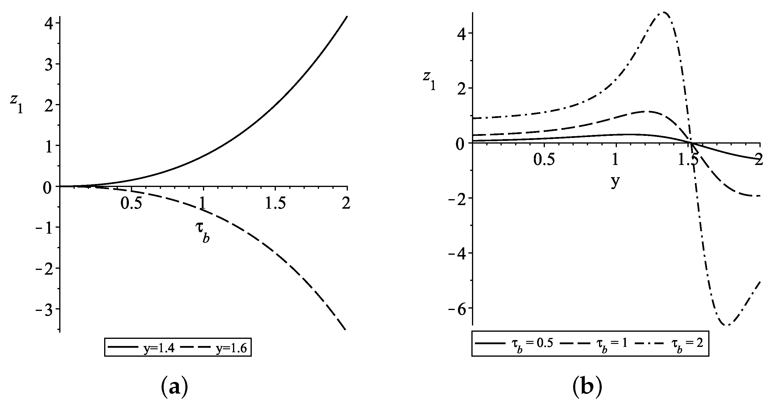
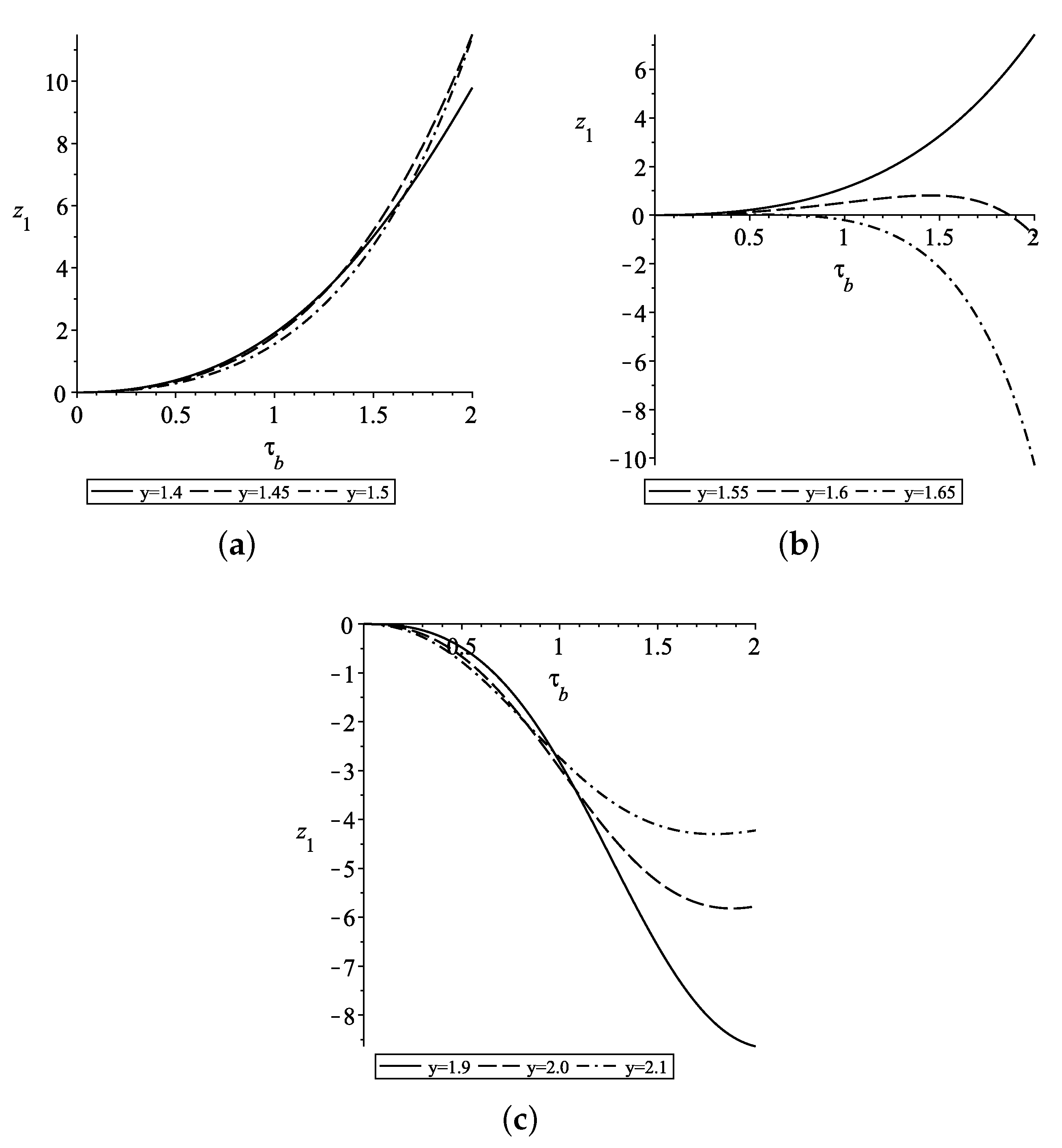
In Figure 6, $z_1$ is plotted as a function of ${\tau }_b$ in [0,2] for various values of y with ${ϵ}_2=25/48$. We see that when $y\le 1.55$, $z_1$ increases as a function of ${\tau }_b$; when $y=1.6,$$z_1$ initially slowly increases before turning to decrease; then, for $1\le {\tau }_b\le 2$ when $y\ge 1.65,$$z_1$ decreases before turning. The larger y is in this last range, the smaller the magnitude of the turning point. Compared with $z_1$ when ${ϵ}_3={ϵ}_2$ and $\gamma =0$, $z_1$ generally increases/decreases more quickly but mostly maintains the same shape.

Subcase $\mathbf{\gamma }=\mathbf{0}.\mathbf{5}$

For $z_1$ when ${ϵ}_3=2{ϵ}_2$ and $\gamma =\frac{1}{2}$, we solve

$${\left(z_1\right)}_{{\tau }_b}=y{\left(z_0\right)}_{yy}+(1-y)(q_2-y)(q_3-y){\left(z_1\right)}_y,$$

(39)

where $q_2=1+{ϵ}_2$ and $q_3=1+3{ϵ}_2$.

Hence,

$$\begin{array}{c}\hfill z_1=-\int \frac{f(y,{\tau }_b)}{(1-y)(q_2-y)(q_3-y)}dy+\psi \left(\xi \right),\end{array}$$

where $f(y,{\tau }_b)=y{\left(z_0\right)}_{yy}$ with $X=e^{-6{ϵ}_2^2{\tau }_b}$ replaced by $\frac{A{(q_2-y)}^3}{{(1-y)}^2(q_3-y)}$ (after ${\left(z_0\right)}_{yy}$ has been determined). The solution process is then the same as in the previous section. Hence, the above work provides the proof for the following proposition:

Proposition 4.

An analytic approximation of (9) with ${ϵ}_2=2{ϵ}_3$ and $\gamma =0.5$ is $z=z_0+ϵz_1$, where $z_0$ is given in (29) and $z_1$ is as given above. Then the futures price is given by $F=F=p_{1}z\left(\frac{p}{p_1},\tau \alpha p_1^2\right).$

In Figure 7, $z_1$ when $\gamma =0.5$ is plotted as a function of ${\tau }_b$ in [0,2] for various values of y with ${ϵ}_2=25/48$. Compared to the case when $\gamma =0$, $z_1$ displays the same behaviour but the magnitude of the values is greater.

In

Table 7. ${ϵ}_3=2{ϵ}_2,\gamma =0.5,{ϵ}_2=\frac{25}{48}$.

y	$({\tau }_b,ϵ)$ = (0.0506, 0.2469)			$({\tau }_b,ϵ)$ = (0.0773, 0.1548)
	$z_0$	$z=z_0+ϵz_1$	FD	$z_0$	$z=z_0+ϵz_1$	FD
1.5	1.4994	1.5000	1.5000	1.4991	1.5000	1.4999
1.6	1.6024	1.6026	1.6026	1.6036	1.6040	1.6040
1.7	1.7056	1.7055	1.7055	1.7086	1.7085	1.7085
1.8	1.8088	1.8083	1.8083	1.8135	1.8128	1.8128
2.1	2.1150	2.1130	2.1133	2.1229	2.1205	2.1204
2.2	2.2149	2.2127	2.2127	2.2227	2.2195	2.2195
RMSE	$1.18\times {10}^{-3}$	$1.2\times {10}^{-4}$		$1.72\times {10}^{-3}$	$6.0\times {10}^{-5}$
MAE	$8.8\times {10}^{-4}$	$5.0\times {10}^{-5}$		$1.28\times {10}^{-3}$	$3.0\times {10}^{-5}$
y	$({\tau }_b,ϵ)$ = (0.1013, 0.2469)			$({\tau }_b,ϵ)$ = (0.1546, 0.1548)
	$z_0$	$z=z_0+ϵz_1$	FD	$z_0$	$z=z_0+ϵz_1$	FD
1.5	1.4988	1.5012	1.5009	1.4982	1.5017	1.5014
1.6	1.6048	1.6059	1.6057	1.6074	1.6092	1.6088
1.7	1.7113	1.7111	1.7109	1.7176	1.7172	1.7169
1.8	1.8178	1.8160	1.8159	1.8276	1.8247	1.8246
2.1	2.1300	2.1231	2.1231	2.1459	2.1356	2.1357
2.2	2.2297	2.2210	2.2210	2.2451	2.2323	2.2325
MAE	$3.48\times {10}^{-3}$	$1.3\times {10}^{-4}$		$5.18\times {10}^{-3}$	$2.3\times {10}^{-4}$
y	$({\tau }_b,ϵ)$ = (0.2025, 0.2469)			$({\tau }_b,ϵ)$ = (0.6627, 0.0361)
	$z_0$	$z=z_0+ϵz_1$	FD	$z_0$	$z=z_0+ϵz_1$	FD
1.5	1.4976	1.5076	1.5053	1.4913	1.5115	1.5074
1.6	1.6100	1.6147	1.6126	1.6374	1.6456	1.6427
1.7	1.7234	1.7221	1.7205	1.7889	1.7811	1.7807
1.8	1.8366	1.8282	1.8276	1.9368	1.9034	1.9149
2.1	2.1602	2.1313	2.1325	2.2928	2.2440	2.2482
2.2	2.2587	2.2237	2.2255	2.3755	2.3267	2.3300
RMSE	$1.84\times {10}^{-2}$	$1.70\times {10}^{-3}$		$2.86\times {10}^{-2}$	$5.57\times {10}^{-3}$
MAE	$1.39\times {10}^{-2}$	$1.60\times {10}^{-3}$		$2.36\times {10}^{-2}$	$4.40\times {10}^{-3}$

we present the results obtained for $z=z_0$ and $z=z_0+ϵz_1$ and those obtained using an implicit finite difference method in Maple [29]. The dimensionless parameters used are given in the table. The results are very similar to those of Table 4, Table 5 and Table 6, with the $O\left(ϵ\right)$ approximations $z=z_0+ϵz_1$ outperforming the $O\left(1\right)$ solutions $z_0$. The RMSE from the $O\left(ϵ\right)$ approximations ranges from $6.0\times {10}^{-5}$ with mostly five-significant-figure accuracy (with ${\tau }_b=0.0773$) to RMSE of $5.57\times {10}^{-3}$ and mostly three-significant-figure accuracy with (${\tau }_b=0.6627$).

4. Conclusions

There are many stochastic models that can be found in the literature that aim to model oil prices. Most have mean-reverting drifts that imply reversion to one mean value. However, examination of historical oil prices points to two basins of attraction. In this paper, we have addressed this fact and modelled the oil price process with a single one-factor nonlinear model that can capture this property. GMM analysis comprehensively indicated that a cubic term was necessary in the drift term in the oil price process, as in our bimodal model. Pricing futures contracts under our model requires solving a partial differential equation for which an exact analytic solution is not available. However, we were able to find analytic approximations for the futures prices that provide fast and accurate solutions. We first non-dimensionalised the governing PDE and found perturbation expansions for the new non-dimensional dependent variable z. The results showed that—while the leading-order approximation $z=z_0$ yielded good results—using the next-order approximation $z=z_0+ϵz_1$ provided even better approximations. Higher-order approximations can be found routinely if necessary, as indicated in Section 3.1.2. There are definite advantages to having an analytic approximation over a numerical answer as it gives faster answers and insight into the general properties of the solution, but, more importantly here, we would be able to calibrate it to oil price data to find the best parameter values to fit the model to price and forecast futures prices. This will be the subject of our next paper: calibration of oil price models to real data and comparing their performance in valuing and forecasting oil price futures. Given that crude oil is, at the moment, the main source of energy production in the world, and given the reliance many investors around the world have on oil futures for the purposes of speculation and management of their portfolios’ risk, we feel that the current paper could provide a better understanding and guidance to investors.

References

1. Brennan, M.; Schwartz, E. Evaluating Natural Resource Investments. J. Bus. 1985, 58, 135–157. [Google Scholar] [CrossRef]
2. Gabillon, J. The Term Structures of Oil Futures Prices; Oxford Institute for Energy Studies: Oxford, UK, 1991. [Google Scholar]
3. Bjerksund, P.; Ekern, S. Contingent claims evaluation of mean-reverting cash flows in shipping. In Real Options in Capital Investment: Models, Strategies, and Applications; Trigeorgis, L., Ed.; Praeger: Westport, Ireland, 1995. [Google Scholar]
4. Schwartz, E. The stochastic behaviour of commodity prices: Implications for valuation and hedging. J. Financ. 1997, 3, 923–973. [Google Scholar] [CrossRef]
5. Pindyck, R. The Long-Run evolutions of energy prices. Energy J. 1999, 20, 1–27. [Google Scholar] [CrossRef]
6. AbaOud, M.; Goard, J. Stochastic Models for Oil Prices and the Pricing of Futures on Oil. Appl. Math. Financ. 2015, 22, 189–206. [Google Scholar] [CrossRef]
7. Gibson, R.; Schwartz, E. Stochastic Conveience Yield And The Pricing of Oil Continget Claims. J. Financ. 1999, 3, 959–976. [Google Scholar]
8. Pilipovic, D. Energy Risk: Valuing and Managing Energy Derivatives; McGraw Hill: New York, NY, USA, 1997. [Google Scholar]
9. Schwartz, E.; Smith, J. Short-Term Variation And Long-Trem Dyanamics in Commodity Prices. Manag. Sci. 2000, 46, 893–911. [Google Scholar] [CrossRef]
10. Hilliard, J.; Reis, J. Valuation of Commodity Futures and Options Under Stochastic Convenience Yield, Interest Rates, and Jump Diffusions in The Spot. J. Financ. Quant. Anal. 1998, 33, 61–86. [Google Scholar] [CrossRef]
11. Cortazar, G.; Schwartz, E. Implementing a Stochastic Model For Oil Futures Prices. Energy Econ. 2003, 25, 215–238. [Google Scholar] [CrossRef]
12. Abadie, L.; Chamorro, J. Valuation of Real Options in Crude Oil Production. Energies. 2017, 10, 1218. [Google Scholar] [CrossRef]
13. Cortazar, J.; Naranjo, L. An N-factor Gaussian model of oil futures prices. J. Futures Mark. 2006, 26, 243–268. [Google Scholar] [CrossRef]
14. Ogbogbo, C. Stochastic Model of Crude Oil Spot Price Process as a Jump-Diffusion Process. Appl. Math. Inf. Sci. 2009, 13, 1029–1037. [Google Scholar]
15. Hayashi, F. Econometrics; Princeton University Press: Princeton, NJ, USA, 2000. [Google Scholar]
16. Mackinlay, A.; Richardson, M. Using Generalized Method of Moments to Test Mean-Variance Efficiency. J. Financ. 1991, 46, 511–526. [Google Scholar] [CrossRef]
17. Ferson, W.; Foerster, S. Finite Sample Properties of the Generalized Method of Moments in Tests of Conditional Asset Pricing Models. J. Financ. Econ. 1994, 36, 29–55. [Google Scholar] [CrossRef]
18. Heston, S. A Simple New Formula for Options with Stochastic Volatility; Olin, J.M., Ed.; School of Business, Washington University: St. Louis, MI, USA, 1997. [Google Scholar]
19. Black, F.; Scholes, M. The Valuation of Option Contracts And a Test of Market Efficiency. J. Financ. 1972, 27, 399–417. [Google Scholar] [CrossRef]
20. McDonald, R.; Siegel, D. Investment and The Valuation of Firms When There Is An Option to Shut Down. Int. Econ. Rev. 1985, 26, 331–349. [Google Scholar] [CrossRef]
21. Goard, J.; Hansen, N. Comparison of the performance of a time-dependent short-interest rate model with time-independent models. Appl. Math. Financ. 2004, 11, 147–164. [Google Scholar] [CrossRef]
22. Goard, J.; Mazur, M. Stochastic volatility models and the pricing of vix options. Math. Financ. 2013, 23, 439–458. [Google Scholar] [CrossRef]
23. Goard, J. A time-dependent variance model for pricing variance and volatility swaps. Appl. Math. Financ. 2011, 18, 51–70. [Google Scholar] [CrossRef]
24. Egloff, D.; Leippold, M.; Wu, L. The Term Structure of Variance Swap Rates and Optimal Variance Swap Investments. J. Fin. Quant. Anal. 2010, 45, 1279–1310. [Google Scholar] [CrossRef]
25. Stein, E.; Stein, J. Stock Price Distributions with Stochastic Volatility: An Analytical Approach. Rev. Finan. Stud. 1991, 4, 727–752. [Google Scholar] [CrossRef]
26. Grünbichler, A.; Longstaff, F. Valuing Futures and Options on Volatility. J. Bank. Financ. 1996, 20, 985–1001. [Google Scholar] [CrossRef]
27. Wilmott, P. Derivatives: The Theory and Practice of Financial Engineering; John Wiley & Sons: Chichester, UK, 1998. [Google Scholar]
28. Debnath, L. Nonlinear Partial Differential Equations for Scientists and Engineers; Birkhäuser: Boston, MA, USA, 2005. [Google Scholar]
29. Maple. Maplesoft; A Division of Waterloo Maple Inc.: Waterloo, ON, Canada, 2018. [Google Scholar]
30. Hansen, L. Large Sample Properties of Generalized Method of Moments Estimators. Econometrica 1982, 50, 1029–1054. [Google Scholar] [CrossRef]
31. Raj, M.; Sim, A.; Thurston, D. A generalized method of moments comparison of the cox-ingersoll-ross and heath-jarrow-morton models. J. Bus. Econ. 1997, 49, 169–192. [Google Scholar] [CrossRef]
32. Hamisultane, H. Utility-based pricing of weather derivatives. Eur. J. Financ. 2009, 16, 503–525. [Google Scholar] [CrossRef]
33. Newey, W.; West, K. A Simple, Positive Semi-Definite, Heteroskedasticity and Autocorrelation Consistent Covariance Matrix. Econometrica 1982, 55, 703–708. [Google Scholar] [CrossRef]
Figure 1. Brent crude oil prices 2011–2022.
Mathematics 11 02222 g001
Figure 2. Plot of z 0 when ϵ 3 = ϵ 2 = 25 / 48 .
Mathematics 11 02222 g002
Figure 3. Plot of z 1 when ϵ 3 = ϵ 2 and γ = 0 .
Mathematics 11 02222 g003
Figure 4. Plot of z 1 when ϵ 3 = ϵ 2 = 25 / 48 and γ = 0.5 .
Mathematics 11 02222 g004
Figure 5. Plot of z 0 when ϵ 2 = 25 / 48 and ϵ 3 = 2 ϵ 2 .
Mathematics 11 02222 g005
Figure 6. Plot of z 1 when ϵ 3 = 2 ϵ 2 and γ = 0 .
Mathematics 11 02222 g006
Figure 7. Plot of z 1 when ϵ 3 = 2 ϵ 2 and γ = 0.5 .
Mathematics 11 02222 g007