Figure 1.
Overview of the proposed method for plant image SRR and classification.
Figure 1.
Overview of the proposed method for plant image SRR and classification.
Figure 2.
Example of preprocessing on thermal image.
Figure 2.
Example of preprocessing on thermal image.
Figure 3.
Preprocessing of visible-light image.
Figure 3.
Preprocessing of visible-light image.
Figure 4.
Detailed structure of PlantSR.
Figure 4.
Detailed structure of PlantSR.
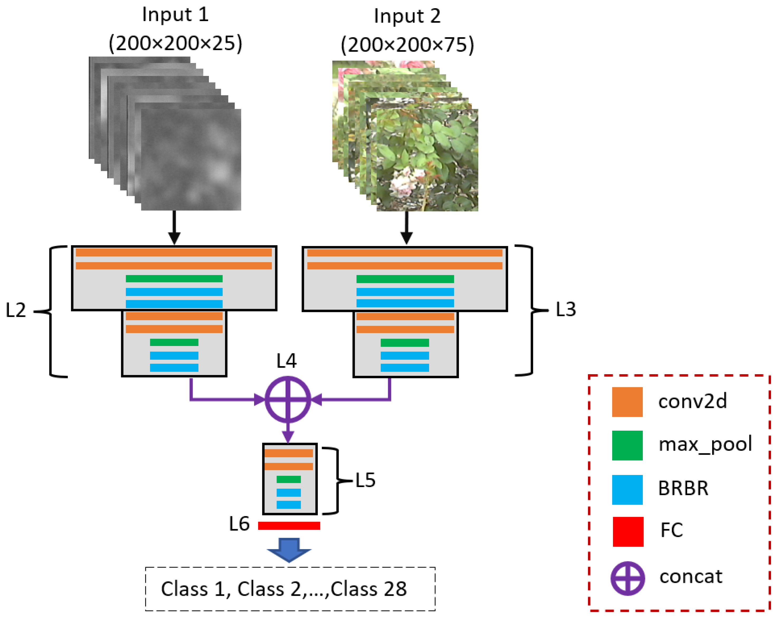
Figure 5.
Detailed structure of PlantMC.
Figure 5.
Detailed structure of PlantMC.
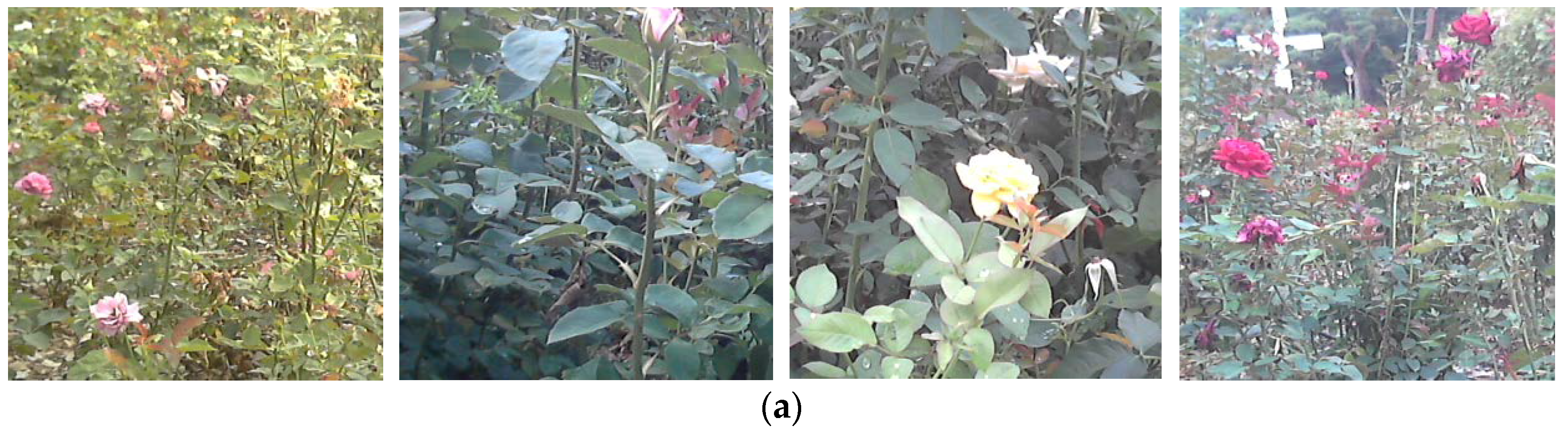
Figure 6.
Example images of TherVisDb. From left to right: images of blue river, charm of Paris, Cleopatra and cocktail. (a) Visible-light images and (b) corresponding thermal images.
Figure 6.
Example images of TherVisDb. From left to right: images of blue river, charm of Paris, Cleopatra and cocktail. (a) Visible-light images and (b) corresponding thermal images.
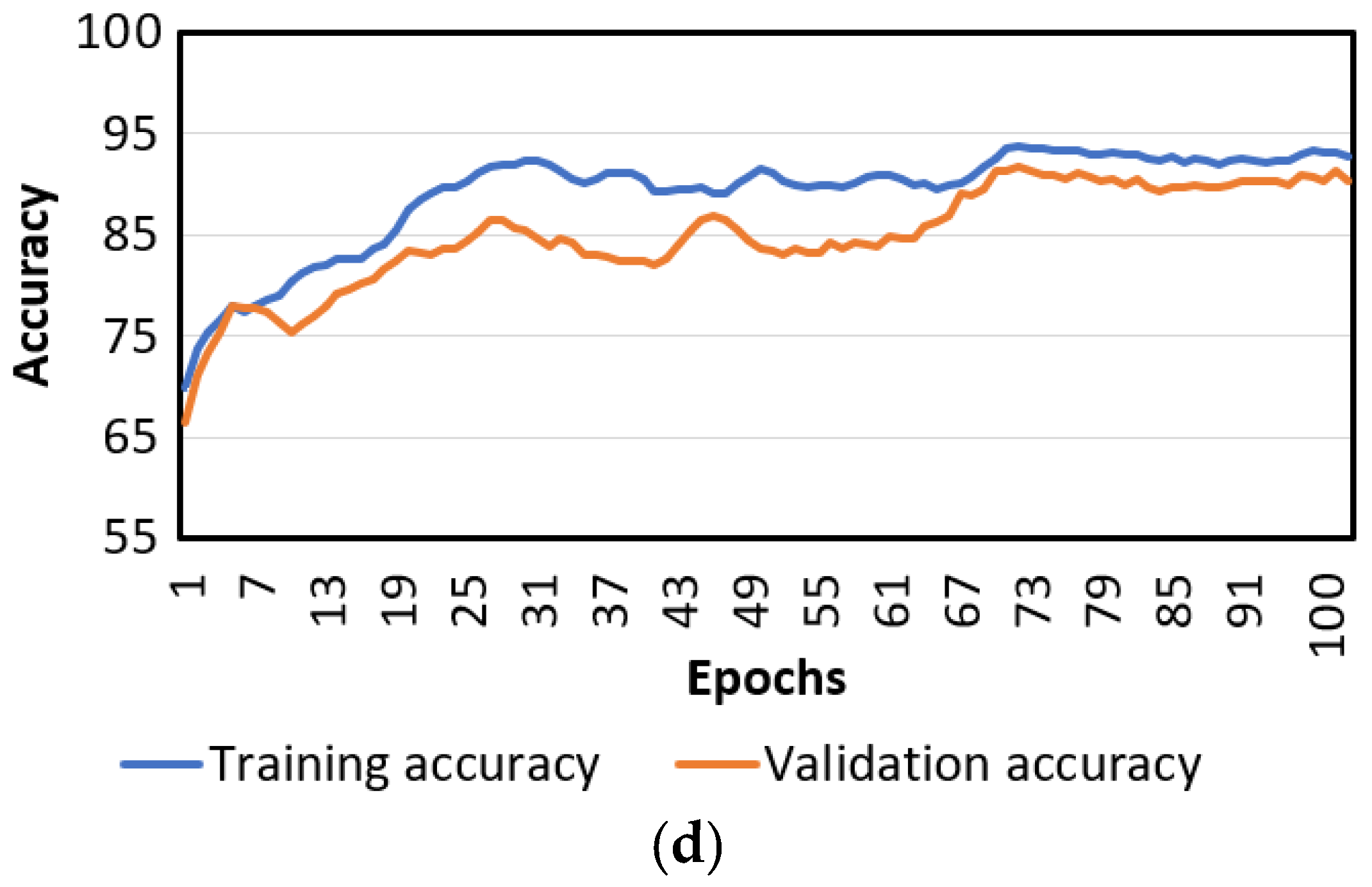
Figure 7.
Loss and accuracy curves of the PlantSR and PlantMC. (a) Training loss curves of PlantSR; (b) validation loss curves of PlantSR; (c) training and validation loss curves of PlantMC; (d) training and validation accuracy curves of PlantMC.
Figure 7.
Loss and accuracy curves of the PlantSR and PlantMC. (a) Training loss curves of PlantSR; (b) validation loss curves of PlantSR; (c) training and validation loss curves of PlantMC; (d) training and validation accuracy curves of PlantMC.
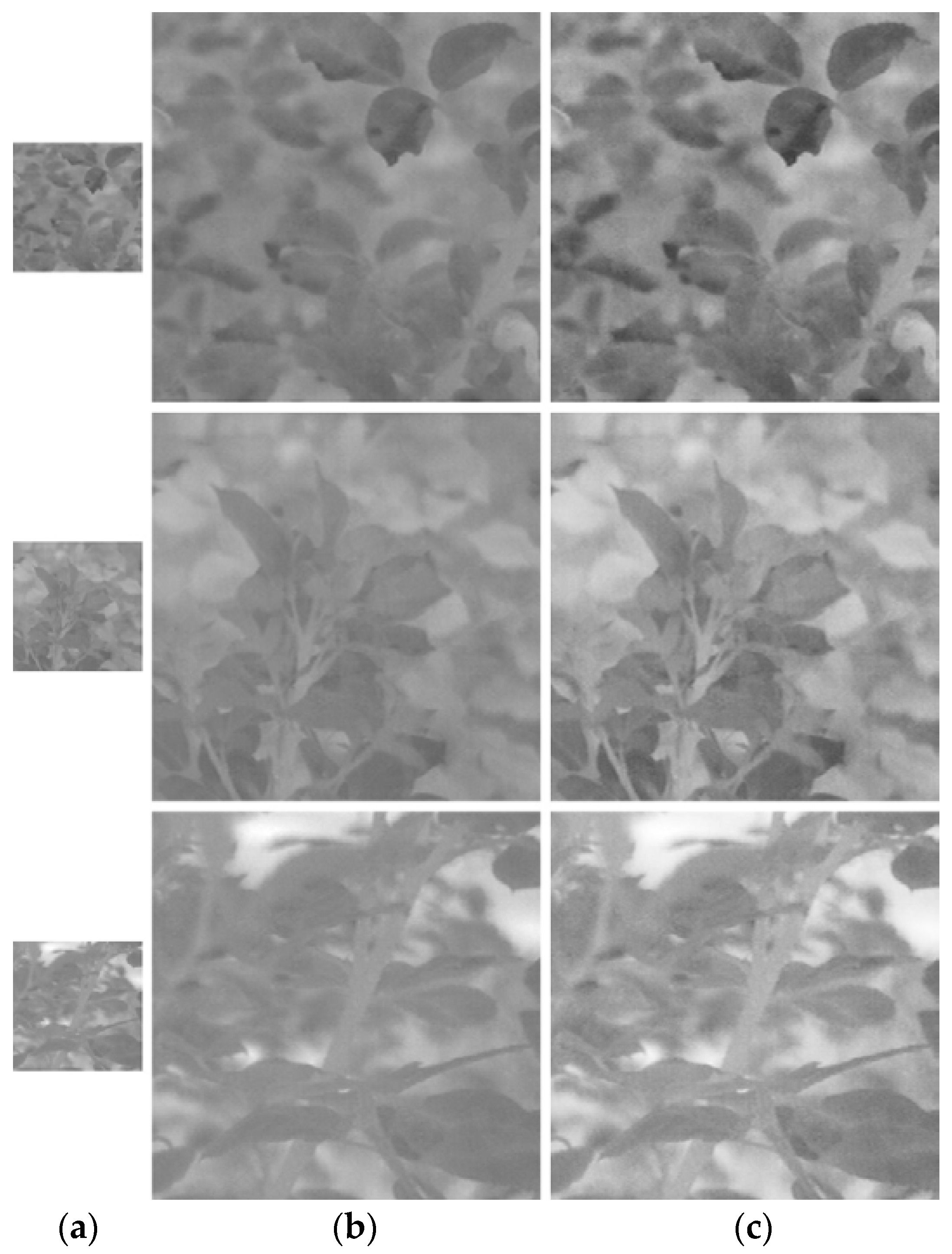
Figure 8.
Example thermal images generated by PlantSR. From top to bottom, images of Rose gaujard, Duftrausch and Elvis. (
a) Original image; (
b) enlarged image by bicubic [
32]; (
c) enlarged image by PlantSR.
Figure 8.
Example thermal images generated by PlantSR. From top to bottom, images of Rose gaujard, Duftrausch and Elvis. (
a) Original image; (
b) enlarged image by bicubic [
32]; (
c) enlarged image by PlantSR.
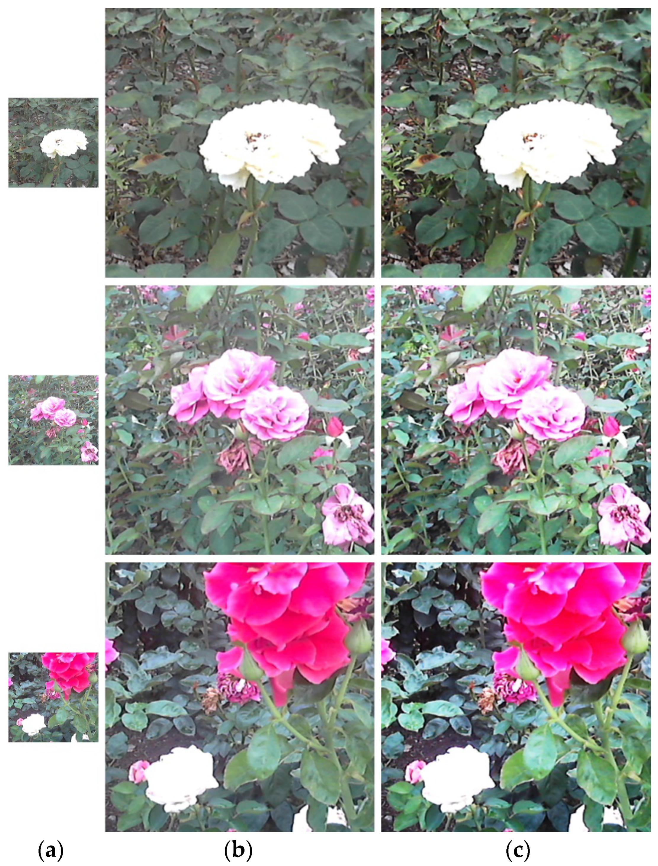
Figure 9.
Example visible-light images generated by PlantSR. From top to bottom, images of White symphonie, Roseraie du chatelet and Twist. (a) Original image; (b) enlarged image by bicubic; (c) enlarged image by PlantSR.
Figure 9.
Example visible-light images generated by PlantSR. From top to bottom, images of White symphonie, Roseraie du chatelet and Twist. (a) Original image; (b) enlarged image by bicubic; (c) enlarged image by PlantSR.
Figure 10.
Example visible-light images generated by SRR methods. From top to bottom, images of White symphonie, Roseraie du chatelet and Twist. (a) Original image; (b) enlarged image by bicubic; (c) enlarged image by Method-1; (d) enlarged image by Method-2; (e) enlarged image by PlantSR.
Figure 10.
Example visible-light images generated by SRR methods. From top to bottom, images of White symphonie, Roseraie du chatelet and Twist. (a) Original image; (b) enlarged image by bicubic; (c) enlarged image by Method-1; (d) enlarged image by Method-2; (e) enlarged image by PlantSR.
Figure 11.
Example of error cases of thermal images generated by PlantSR. From top to bottom, images of Rose gaujard, Duftrausch and Elvis. (a) Original image; (b) enlarged image by bicubic; (c) enlarged image by PlantSR.
Figure 11.
Example of error cases of thermal images generated by PlantSR. From top to bottom, images of Rose gaujard, Duftrausch and Elvis. (a) Original image; (b) enlarged image by bicubic; (c) enlarged image by PlantSR.
Figure 12.
Example of error cases of visible-light images generated by PlantSR. From top to bottom, images of White symphonie, Roseraie du chatelet and Twist. (a) Original image; (b) enlarged image by bicubic; (c) enlarged image by PlantSR.
Figure 12.
Example of error cases of visible-light images generated by PlantSR. From top to bottom, images of White symphonie, Roseraie du chatelet and Twist. (a) Original image; (b) enlarged image by bicubic; (c) enlarged image by PlantSR.
Table 1.
Summary of existing classification and SRR studies on plant image databases.
Table 1.
Summary of existing classification and SRR studies on plant image databases.
| Categories | Modalities | Tasks | Methods | Advantages | Disadvantages |
|---|
| Classification without SRR | Visible-light image-based | Multiclass classification | AAR network [2], DenseNet-121 [3], OMNCNN [4], CNNs [5], T-CNN [6], and PI-CNN [9] | - −
Provides high-quality (HQ) image in both day and high illumination environment - −
Provides color information - −
Extracts features automatically - −
Considers multiclass problem
| - −
Provides dark image in a nighttime or low illumination environment - −
Provides low-quality (LQ) image in both day and high illumination environment owing to shadow, illumination change, ambient light, and its reflection.
|
| Thermal image-based | Multiclass
classification | PlantDXAI [10] | - −
Provides thermal information - −
Extracts features automatically - −
Considers multiclass problem
| - −
Does not provide color information - −
Sensitive to temperature and humidity of the environment
|
| Thermal and visible-light images-based | Binary
classification | SVM [11] | - −
Provides HQ image in both day and high illumination environment - −
Provides color and thermal information
| - −
Very challenging to extract appropriate features - −
Does not consider multiclass problem - −
Computationally expensive owing to use of three camera sensors
|
Multiclass
classification | PlantCR [14] | - −
Provides HQ image in both day and high illumination environment - −
Provides color and thermal information - −
Extracts features automatically - −
Considers multiclass problem
| Computationally expensive owing to use of two camera sensors |
| Classification with SRR | Visible-light image-based | Multiclass
classification | Modified SRCNN + AlexNet [15],
GAN-based SRR +
CNNDiag [16] | - −
Provides HR and HQ image in both day and high illumination environment - −
Provides color information - −
Higher performance by using classification with SRR - −
Extracts features automatically - −
Considers multiclass problem
| - −
Provides dark image in nighttime or low illumination environment - −
Provides LQ image in both day and high illumination environment owing to shadow, illumination change, ambient light, and its reflection.
|
| Thermal and visible-light images-based | Multiclass
classification | PlantSR + PlantMC (Proposed method) | - −
Provides HR and HQ image in both day and high illumination environment - −
Provides thermal and color information - −
Higher performance by using classification with SRR - −
Extracts features automatically - −
Considers multiclass problem
| Computationally expensive owing to use of two camera sensors |
Table 2.
Description of the generator network of PlantSR.
Table 2.
Description of the generator network of PlantSR.
| Layer# | Layer Type | Filter# | Parameter# | Layer Connection |
|---|
| 1 | input layer | 0 | 0 | input |
| 2 | group_1 | 128 | 741,760 | input layer |
| 3 | Up3 | 0 | 0 | group_1 |
| 4 | group_2 | 64 | 258,560 | Up3 |
| 5 | conv2d (tanh) | X | 1,731 | group_2 |
| | Total number of trainable parameters: 1,002,051 |
Table 3.
Description of the discriminator network of PlantSR.
Table 3.
Description of the discriminator network of PlantSR.
| Layer# | Layer Type | Filter# | Parameter# | Layer Connection |
|---|
| 1 | input layer | 0 | 0 | input |
| 2 | group_1 | 64 | 334,400 | input layer |
| 3 | group_2 | 64 | 369,536 | group_1 |
| 4 | LReLU | 0 | 0 | group_2 |
| 5 | FC (sigmoid) | Class# | 1,382,977 | LReLU |
| | Total number of trainable parameters: 2,086,913 |
Table 4.
Group layer of generator network.
Table 4.
Group layer of generator network.
| Times | Layer Type | Layer Connection |
|---|
| 1 | input layer | input |
| 2 | conv2d | input layer |
| 1 | RBRB | conv2d |
Table 5.
Group layer of discriminator network.
Table 5.
Group layer of discriminator network.
| Times | Layer Type | Layer Connection |
|---|
| 1 | input layer | input |
| 2 | conv2d | input layer |
| 1 | max_pool | conv2d |
| 2 | RBRB | max_pool |
Table 6.
Description of RBRB.
Table 6.
Description of RBRB.
| Layer Type | Layer Connection |
|---|
| input layer | input |
| res_block_1 | input layer |
| res_block_2 | res_block_1 |
| add | res_block_2 & input layer |
Table 7.
Description of a residual block.
Table 7.
Description of a residual block.
| Layer Type | Layer Connection |
|---|
| input layer | input |
| conv2d_1 | input layer |
| prelu | conv2d_1 |
| conv2d_2 | prelu |
| add | conv2d_2 & input layer |
Table 8.
Description of the proposed PlantMC.
Table 8.
Description of the proposed PlantMC.
| Layer# | Times | Layer Type | Filter# | Parameter# | Layer Connection |
|---|
| 1 | 1 | input layer_1 & 2 | 0 | 0 | 0 | input |
| 2 | 2 | group_1 | 64/128 | 1,735,872 | 1,749,696 | input layer_1 |
| 3 | 2 | group_2 | 64/128 | 1,737,024 | 1,778,496 | input layer_2 |
| 4 | 1 | concat | 0 | 0 | 0 | group_1 & group_2 |
| 5 | 1 | group_3 | 128 | 1,623,808 | 1,623,808 | concat |
| 6 | 1 | FC (softmax) | class# | 229,404 | 14,364 | group_3 |
| Total number of trainable parameters: 5,326,108/5,166,364 |
Table 9.
Description of classes and dataset split.
Table 9.
Description of classes and dataset split.
| Class Index | Class Names | Image# | Thermal Image# | Visible-Light Image# | Set 1 | Set 2 | Set 3 | Validation Set |
|---|
| 1 | Alexandra | 240 | 120 | 120 | 72 | 72 | 72 | 24 |
| 2 | Belvedere | 96 | 48 | 48 | 28 | 28 | 28 | 12 |
| 3 | Blue river | 272 | 136 | 136 | 82 | 82 | 82 | 26 |
| 4 | Charm of paris | 272 | 136 | 136 | 82 | 82 | 82 | 26 |
| 5 | Cleopatra | 304 | 152 | 152 | 88 | 88 | 88 | 40 |
| 6 | Cocktail | 224 | 112 | 112 | 70 | 70 | 70 | 14 |
| 7 | Duftrausch | 352 | 176 | 176 | 104 | 104 | 104 | 40 |
| 8 | Echinacea sunset | 128 | 64 | 64 | 38 | 38 | 38 | 14 |
| 9 | Eleanor | 288 | 144 | 144 | 88 | 88 | 88 | 24 |
| 10 | Elvis | 448 | 224 | 224 | 134 | 134 | 134 | 46 |
| 11 | Fellowship | 416 | 208 | 208 | 124 | 124 | 124 | 44 |
| 12 | Goldeise | 288 | 144 | 144 | 86 | 86 | 86 | 30 |
| 13 | Goldfassade | 368 | 184 | 184 | 112 | 112 | 112 | 32 |
| 14 | Grand classe | 528 | 264 | 264 | 158 | 158 | 158 | 54 |
| 15 | Just joey | 144 | 72 | 72 | 42 | 42 | 42 | 18 |
| 16 | Kerria japonica | 208 | 104 | 104 | 62 | 62 | 62 | 22 |
| 17 | Margaret | 224 | 112 | 112 | 66 | 66 | 66 | 26 |
| 18 | Oklahoma | 624 | 312 | 312 | 186 | 186 | 186 | 66 |
| 19 | Pink perfume | 240 | 120 | 120 | 72 | 72 | 72 | 24 |
| 20 | Queen elizabeth | 240 | 120 | 120 | 72 | 72 | 72 | 24 |
| 21 | Rose gaujard | 624 | 312 | 312 | 186 | 186 | 186 | 66 |
| 22 | Rosenau | 608 | 304 | 304 | 182 | 182 | 182 | 62 |
| 23 | Roseraie du chatelet | 704 | 352 | 352 | 214 | 214 | 214 | 62 |
| 24 | Spiraea salicifolia l | 128 | 64 | 64 | 38 | 38 | 38 | 14 |
| 25 | Stella de oro | 96 | 48 | 48 | 28 | 28 | 28 | 12 |
| 26 | Twist | 576 | 288 | 288 | 172 | 172 | 172 | 60 |
| 27 | Ulrich brunner fils | 240 | 120 | 120 | 72 | 72 | 72 | 24 |
| 28 | White symphonie | 560 | 280 | 280 | 168 | 168 | 168 | 56 |
| Total | 9440 | 4720 | 4720 | 2826 | 2826 | 2826 | 962 |
Table 10.
Weather information for the surrounding environment at the time of image acquisition.
Table 10.
Weather information for the surrounding environment at the time of image acquisition.
| Types of Weather Measurement | Numerical Values with Units |
|---|
| Humidity | 91% |
| Temperature | 30 °C |
| Wind speed | 3 m/s |
| Fine dust | 24 μg/m3 |
| Ultra-fine dust | 22 μg/m3 |
| UV index | 8 |
Table 11.
Other relevant information in the dataset.
Table 11.
Other relevant information in the dataset.
| Lists | Thermal
Image | Visible Light
Image | Units |
|---|
Before
augmentation | Image size | 640 × 512 × 1 | 640 × 512 × 3 | pixel |
| Depth | 14 | 24 | bit |
| Class number | 28 | 28 | - |
| Image extension | bmp | bmp | - |
| Camera sensor | Flir Tau® 2 [19] | Logitech C270 [20] | - |
After
augmentation | Image size | 300 × 300 × 1 | 300 × 300 × 3 | pixel |
| Depth | 8 | 24 | bit |
| Image extension | png | png | - |
Table 12.
Description of hardware and software of desktop computer.
Table 12.
Description of hardware and software of desktop computer.
| Hardware | Software |
|---|
| Library (Version) |
|---|
| Processor | Intel(R) Core(TM) i7-6700 CPU@3.40 GHz
(8 CPUs) | OpenCV [21] (4.3.0),
Python [22] (3.5.4),
Keras API [23] (2.1.6-tf),
TensorFlow [24] (1.9.0) |
| Main memory | 32 GB RAM |
| GPU | Nvidia GeForce GTX TITAN X (12 GB) |
Table 13.
Search spaces and selected values of hyperparameters for the proposed methods.
Table 13.
Search spaces and selected values of hyperparameters for the proposed methods.
| Parameters | PlantSR | PlantMC |
|---|
| Search Space | Selected Value | Search Space | Selected Value |
|---|
| Learning rate | [0.00001, 0.0001, 0.001] | 0.0001 | [0.00001, 0.0001, 0.001] | 0.0001 |
| Epochs | [1~100] | 92 | [1~100] | 74 |
| Batch size | [1, 8, 16] | 8 | [1, 8, 16] | 8 |
| Optimizer | Adam [25] | Adam | Adam | Adam |
| Loss | binary cross-entropy [26] | binary cross-entropy | categorical cross-entropy [27] | categorical cross-entropy |
Table 14.
Comparison of accuracies obtained in different folds using PlantSR + PlantMC.
Table 14.
Comparison of accuracies obtained in different folds using PlantSR + PlantMC.
| Methods | PPV | TPR | F1-Score | ACC |
|---|
| Fold-1 | 91.25 | 91.46 | 91.46 | 99.94 |
| Fold-2 | 90.26 | 89.86 | 89.61 | 98.82 |
| Fold-3 | 90.08 | 89.73 | 89.40 | 98.90 |
| Average | 90.53 | 90.35 | 90.16 | 99.22 |
Table 15.
Comparison of accuracies obtained by using classification methods with and without RBRB.
Table 15.
Comparison of accuracies obtained by using classification methods with and without RBRB.
| Methods | PPV | TPR | F1-Score | ACC |
|---|
| PlantMC without RBRB | 89.47 | 90.11 | 89.75 | 98.21 |
| PlantMC with RBRB | 90.53 | 90.35 | 90.16 | 99.22 |
Table 16.
Comparison of accuracies obtained using classification methods using images with different sizes and channels.
Table 16.
Comparison of accuracies obtained using classification methods using images with different sizes and channels.
| Methods | PPV | TPR | F1-Score | ACC |
|---|
| PlantMC using 600 × 600 × 1 (3) | 90.4 | 90.45 | 90.1 | 99.21 |
| PlantMC using 200 × 200 × 25 (75) | 90.53 | 90.35 | 90.16 | 99.22 |
Table 17.
Detailed accuracy of each class by the proposed PlantSR and PlantMC with and without PlantSR.
Table 17.
Detailed accuracy of each class by the proposed PlantSR and PlantMC with and without PlantSR.
| # | Class Names | PlantSR (Th) | PlantSR (V) | PlantMC | PlantSR + PlantMC |
|---|
| PSNR | SSIM | PSNR | SSIM | PPV | TPR | F1-Score | ACC | PPV | TPR | F1-Score | ACC |
|---|
| 1 | Alexandra | 26.87 | 0.87 | 27.41 | 0.88 | 91.48 | 99.39 | 95.27 | 99.43 | 92.32 | 99.52 | 95.79 | 100 |
| 2 | Belvedere | 26.59 | 0.89 | 28.18 | 0.88 | 99.68 | 82.73 | 90.42 | 98.95 | 100 | 83.69 | 91.19 | 99.75 |
| 3 | Blue river | 27.27 | 0.86 | 27.6 | 0.95 | 92.61 | 83.19 | 87.65 | 99.24 | 93.23 | 84.17 | 88.47 | 100 |
| 4 | Charm of paris | 27 | 0.84 | 27.46 | 0.87 | 81.52 | 85 | 83.22 | 98.66 | 81.74 | 85.9 | 83.77 | 99.63 |
| 5 | Cleopatra | 27.3 | 0.92 | 27.67 | 0.89 | 57.59 | 94.7 | 71.62 | 98.37 | 58.43 | 95.05 | 72.37 | 98.55 |
| 6 | Cocktail | 27.12 | 0.93 | 27.57 | 0.95 | 90.31 | 90.66 | 90.49 | 99.2 | 91.08 | 91.54 | 91.31 | 99.76 |
| 7 | Duftrausch | 27.36 | 0.93 | 27.8 | 0.93 | 93.58 | 96.76 | 95.14 | 99.02 | 94.15 | 97.17 | 95.64 | 99.19 |
| 8 | Echinacea sunset | 27.42 | 0.9 | 28.14 | 0.85 | 91.94 | 91.63 | 91.79 | 99.22 | 92.43 | 91.95 | 92.19 | 99.54 |
| 9 | Eleanor | 27.4 | 0.91 | 27.9 | 0.87 | 99.18 | 99.57 | 99.38 | 99.99 | 99.63 | 100 | 99.95 | 100 |
| 10 | Elvis | 27.12 | 0.9 | 27.93 | 0.92 | 92.9 | 85.39 | 88.99 | 98.12 | 93.66 | 86.36 | 89.86 | 98.98 |
| 11 | Fellowship | 26.88 | 0.88 | 28.02 | 0.86 | 89.51 | 85.98 | 87.71 | 98.51 | 89.72 | 85.98 | 87.81 | 99.47 |
| 12 | Goldeise | 27.41 | 0.92 | 27.68 | 0.92 | 92.75 | 81.46 | 86.74 | 98.5 | 93.44 | 82.16 | 87.44 | 99.35 |
| 13 | Goldfassade | 27.08 | 0.91 | 27.58 | 0.88 | 91.51 | 86.96 | 89.18 | 99.16 | 91.63 | 87.56 | 89.55 | 99.9 |
| 14 | Grand classe | 27.24 | 0.85 | 28.13 | 0.89 | 81.11 | 85.5 | 83.24 | 97.44 | 81.4 | 85.54 | 83.42 | 97.89 |
| 15 | Just joey | 27.4 | 0.89 | 27.84 | 0.92 | 86.45 | 76.46 | 81.14 | 98.62 | 87.25 | 76.96 | 81.78 | 98.83 |
| 16 | Kerria japonica | 27.11 | 0.89 | 27.38 | 0.94 | 99.89 | 99.37 | 99.63 | 99.22 | 100 | 100 | 100 | 99.26 |
| 17 | Margaret | 27.18 | 0.91 | 27.91 | 0.93 | 82.59 | 86.1 | 84.31 | 98.87 | 83.47 | 86.62 | 85.02 | 99.45 |
| 18 | Oklahoma | 26.47 | 0.86 | 27.97 | 0.93 | 91.89 | 86.19 | 88.95 | 98.5 | 92.40 | 87.06 | 89.65 | 98.68 |
| 19 | Pink perfume | 27.37 | 0.87 | 27.48 | 0.88 | 83.17 | 90.54 | 86.7 | 98.46 | 83.37 | 91.27 | 87.14 | 98.54 |
| 20 | Queen elizabeth | 27.05 | 0.92 | 28.15 | 0.91 | 95.81 | 95.31 | 95.56 | 98.97 | 96.78 | 95.63 | 96.2 | 99.65 |
| 21 | Rose gaujard | 26.66 | 0.87 | 27.8 | 0.91 | 91.88 | 84.31 | 87.93 | 98.06 | 92.84 | 85.25 | 88.88 | 98.4 |
| 22 | Rosenau | 26.73 | 0.88 | 27.69 | 0.93 | 99.46 | 90.05 | 94.52 | 98.42 | 99.8 | 90.95 | 95.17 | 98.47 |
| 23 | Roseraie du chatelet | 26.89 | 0.85 | 28.2 | 0.94 | 82.28 | 94.23 | 87.85 | 97.95 | 82.75 | 94.33 | 88.16 | 98.06 |
| 24 | Spiraea salicifolia l | 27.44 | 0.89 | 28.21 | 0.95 | 99.73 | 99.38 | 99.55 | 99.47 | 99.84 | 99.75 | 99.8 | 100 |
| 25 | Stella de oro | 27.09 | 0.84 | 27.78 | 0.89 | 99.42 | 90.33 | 94.66 | 98.93 | 99.96 | 91.12 | 95.34 | 99.4 |
| 26 | Twist | 26.51 | 0.84 | 28.05 | 0.88 | 90.51 | 94.44 | 92.43 | 98.28 | 91.45 | 94.51 | 92.96 | 98.93 |
| 27 | Ulrich brunner fils | 26.67 | 0.84 | 27.64 | 0.94 | 78.88 | 86.04 | 82.31 | 98.77 | 79.35 | 86.83 | 82.92 | 99.13 |
| 28 | White symphonie | 27.29 | 0.88 | 28.33 | 0.9 | 92.46 | 92.17 | 92.31 | 98.34 | 92.77 | 92.94 | 92.85 | 99.23 |
| | Average | 27.07 | 0.88 | 27.84 | 0.91 | 90 | 89.78 | 89.6 | 98.74 | 90.53 | 90.35 | 90.16 | 99.22 |
Table 18.
Comparison of accuracies by bicubic and the proposed PlantSR, and PlantMC with bicubic and PlantSR.
Table 18.
Comparison of accuracies by bicubic and the proposed PlantSR, and PlantMC with bicubic and PlantSR.
| Images | SRR | PlantMC | SRR + PlantMC |
|---|
| PSNR | SSIM | PPV | TPR | F1-Score | ACC | PPV | TPR | F1-Score | ACC |
|---|
| Original images | - | - | 90 | 89.78 | 89.6 | 98.74 | - | - | - | - |
| Bicubic (Th) | 27 | 0.86 | - | - | - | - | 90.05 | 89.97 | 89.87 | 98.9 |
| Bicubic (V) | 27.7 | 0.89 | - | - | - | - |
| PlantSR (Th) | 27.07 | 0.88 | - | - | - | - | 90.53 | 90.35 | 90.16 | 99.22 |
| PlantSR (V) | 27.84 | 0.91 | - | - | - | - |
Table 19.
Comparison of accuracies obtained by using SRR methods.
Table 19.
Comparison of accuracies obtained by using SRR methods.
| Methods | PSNR | SSIM |
|---|
| Bicubic | 27.7 | 0.89 |
| Method-1 [15] | 27.71 | 0.88 |
| Method-2 [16] | 27.73 | 0.89 |
| PlantMC | 27.84 | 0.91 |
Table 20.
Comparison of accuracies obtained by using classification methods without SRR.
Table 20.
Comparison of accuracies obtained by using classification methods without SRR.
| Methods | PPV | TPR | F1-Score | ACC |
|---|
| Method-1 [15] | 88.13 | 89.49 | 88.71 | 98.21 |
| Method-2 [16] | 88.93 | 89.07 | 89.03 | 98.66 |
| PlantMC | 90 | 89.78 | 89.6 | 98.74 |
Table 21.
Comparison of accuracies obtained by using classification methods with SRR.
Table 21.
Comparison of accuracies obtained by using classification methods with SRR.
| Methods | PPV | TPR | F1-Score | ACC |
|---|
| Method-1 with SRR [15] | 89.39 | 90.12 | 89.98 | 98.79 |
| Method-2 with SRR [16] | 89.75 | 90.21 | 90.05 | 99.1 |
| PlantSR + PlantMC | 90.53 | 90.35 | 90.16 | 99.22 |
Table 22.
Processing time of the methods per image (unit: ms).
Table 22.
Processing time of the methods per image (unit: ms).
| Database | Processing Time |
|---|
| PlantSR using thermal image | 68.45 |
| PlantSR using visible-light image | 62.75 |
| PlantMC using 600 × 600 × 1 (3) | 58.24 |
| PlantMC using 200 × 200 × 25 (75) | 46.12 |
| PlantSRs + PlantMC using 200 × 200 × 25 (75) | 177.32 |


