

Describing Water Wave Propagation Using the


Abstract
:1. Introduction
2. The Basic Idea of the –Expansion Method
3. Application of the –Expansion Method for Equations (1) and (4)
3.1. Modulation Instability Analysis
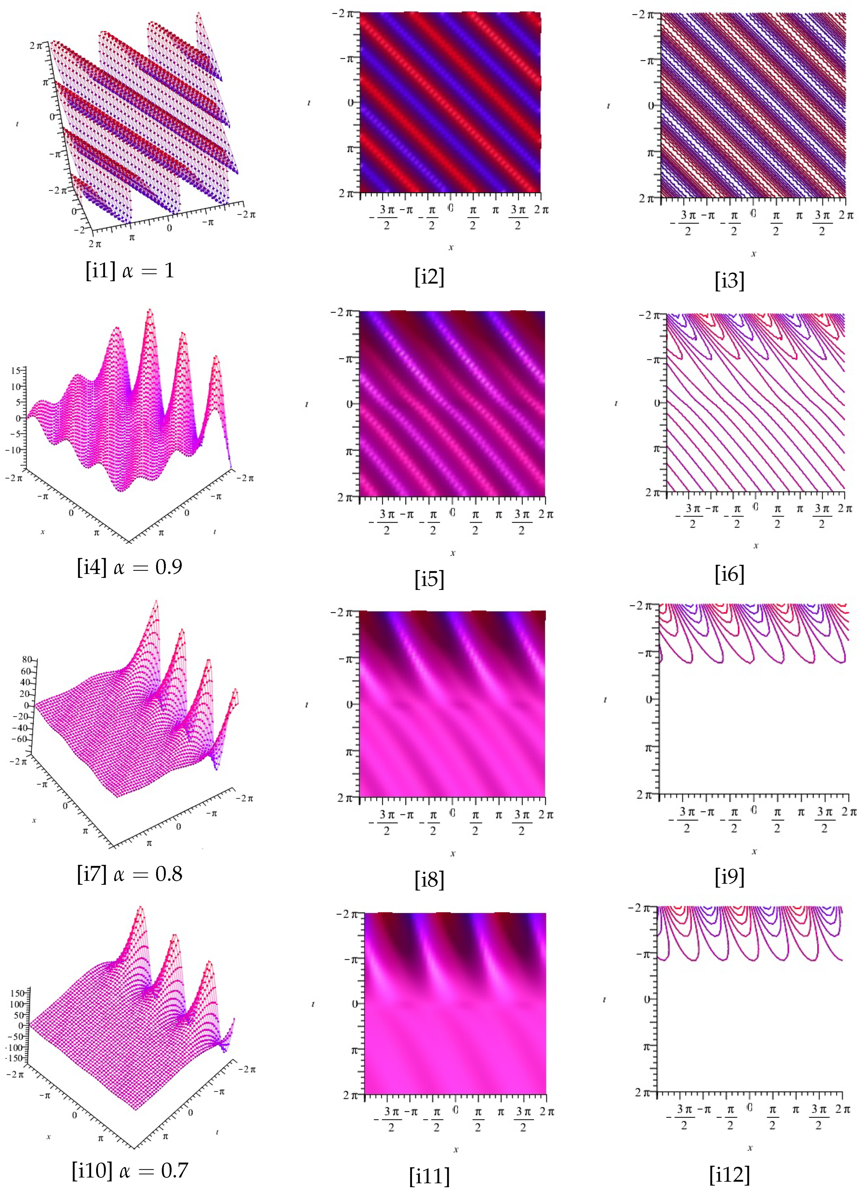
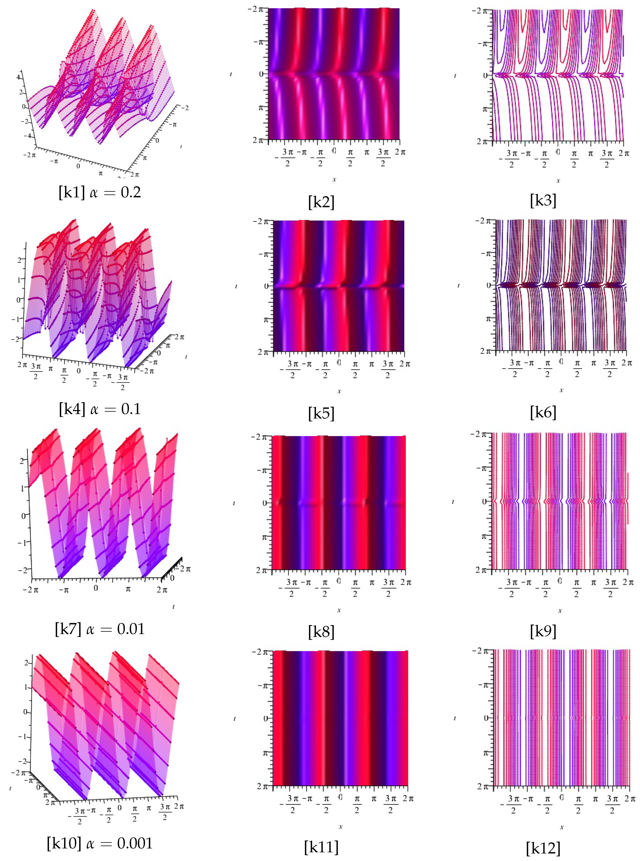
3.2. Discussion
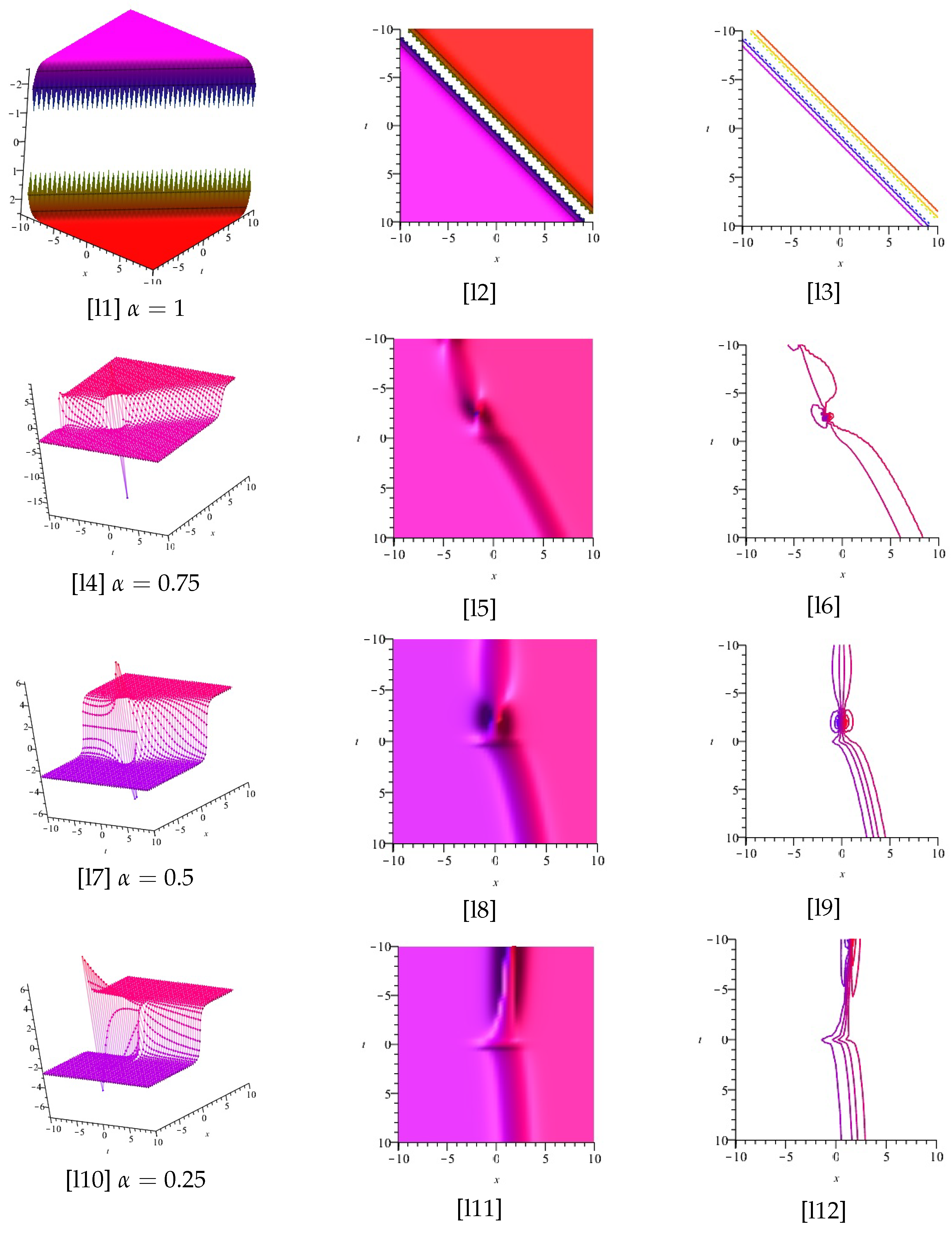
4. Application of the –Expansion Method for Equation (5)
5. Conclusions
Author Contributions
Funding
Data Availability Statement
Acknowledgments
Conflicts of Interest
References
- Rezapour, S.; Günay, B.; Al Shamsi, H.; Nonlaopon, K. On soliton solutions of a modified nonlinear Schrödinger’s equation of third-order governing in optical fibers. Results Phys. 2022, 41, 105919. [Google Scholar] [CrossRef]
- Al-Askar, F.M.; Mohammed, W.W.; Albalahi, A.M.; El-Morshedy, M. The influence of noise on the solutions of fractional stochastic bogoyavlenskii equation. Fractal Fract. 2022, 6, 156. [Google Scholar] [CrossRef]
- Aderyani, S.R.; Saadati, R.; Abdeljawad, T.; Mlaiki, N. Multi-stability of non homogenous vector-valued fractional differential equations in matrix-valued Menger spaces. Alex. Eng. J. 2022, 61, 10913–10923. [Google Scholar] [CrossRef]
- Guo, W.; Yang, Z.; Feng, Q.; Dai, C.; Yang, J.; Lei, X. A new method for band gap analysis of periodic structures using virtual spring model and energy functional variational principle. Mech. Syst. Signal Process. 2022, 168, 108634. [Google Scholar] [CrossRef]
- Hu, J.Y.; Feng, X.B.; Yang, Y.F. Optical envelope patterns perturbation with full nonlinearity for Gerdjikov–Ivanov equation by trial equation method. Optik 2021, 240, 166877. [Google Scholar] [CrossRef]
- Elmandouh, A.A.; Elbrolosy, M.E. New traveling-wave solutions for Gilson-Pickering equation in plasma via bifurcation analysis and direct method. Math. Methods Appl. Sci. 2022. [Google Scholar] [CrossRef]
- Urazboev, G.U.; Baltaeva, I.I.; Rakhimov, I.D. The Generalized (G′/G)-Expansion Method for the Loaded Korteweg–de Vries Equation. J. Appl. Ind. Math. 2021, 15, 679–685. [Google Scholar] [CrossRef]
- Aderyani, S.R.; Saadati, R.; Vahidi, J.; Allahviranloo, T. The exact solutions of the conformable time-fractional modified nonlinear Schrödinger equation by the Trial equation method and modified Trial equation method. Adv. Math. Phys. 2022, 2022, 4318192. [Google Scholar] [CrossRef]
- Alam, M.N.; Tunç, C. The new solitary wave structures for the (2 + 1)-dimensional time-fractional Schrodinger equation and the space–time nonlinear conformable fractional Bogoyavlenskii equations. Alex. Eng. J. 2020, 59, 2221–2232. [Google Scholar] [CrossRef]
- Wang, K.J.; Shi, F.; Liu, J.H.; Si, J. Application of the extended F-expansion method for solving the fractional Gardner equation with conformable fractional derivative. Fractals 2022, 30, 1–11. [Google Scholar] [CrossRef]
- Chen, Q.; Baskonus, H.M.; Gao, W.; Ilhan, E. Soliton theory and modulation instability analysis: The Ivancevic option pricing model in economy. Alex. Eng. J. 2022, 61, 7843–7851. [Google Scholar] [CrossRef]
- Radhakrishnan, B.; Tamilarasi, M. A new approach for the generalized fractional Casson fluid model with Newtonian heating described by the modified Riemann-Liouville fractional operator. Math. Methods Appl. Sci. 2022, 45, 3574–3588. [Google Scholar] [CrossRef]


| 0.012 | 0.012 | 0.00000 | ±0.41523 | 0.00000 | ±339.37846 |
| 0.037 | 0.00000 | ±0.39534 | 0.00000 | ±60.70046 | |
| 0.062 | 0.00000 | ±0.37942 | 0.00000 | ±34.48412 | |
| 0.087 | 0.00000 | ±0.36610 | 0.00000 | ±24.41456 | |
| 0.037 | 0.012 | 0.00000 | ±0.43195 | 0.00000 | ∓143.18583 |
| 0.037 | 0.00000 | ±0.40963 | 0.00000 | ±152.62498 | |
| 0.062 | 0.00000 | ±0.39181 | 0.00000 | ±52.34274 | |
| 0.087 | 0.00000 | ±0.37694 | 0.00000 | ±32.14308 | |
| 0.062 | 0.012 | 0.00000 | ±0.45078 | 0.00000 | ∓59.15192 |
| 0.037 | 0.00000 | ±0.42565 | 0.00000 | ∓295.98183 | |
| 0.062 | 0.00000 | ±0.40568 | 0.00000 | ±108.85178 | |
| 0.087 | 0.00000 | ±0.38904 | 0.00000 | ±47.11727 | |
| 0.087 | 0.012 | 0.00000 | ±0.47207 | 0.00000 | ∓37.30504 |
| 0.037 | 0.00000 | ±0.44368 | 0.00000 | ∓75.16017 | |
| 0.062 | 0.00000 | ±0.42122 | 0.00000 | ∓1346.22816 | |
| 0.087 | 0.00000 | ±0.40258 | 0.00000 | ±88.41972 | |
| 0.012 | 0.012 | 0.00000 | ±1.69922 | 0.00000 | ∓0.01884 |
| 0.037 | 0.00000 | ±1.78472 | 0.00000 | ∓0.10537 | |
| 0.062 | 0.00000 | ±1.85962 | 0.00000 | ∓0.18548 | |
| 0.087 | 0.00000 | ±1.92724 | 0.00000 | ∓0.26198 | |
| 0.037 | 0.012 | 0.00000 | ±1.63346 | 0.00000 | ±0.04467 |
| 0.037 | 0.00000 | ±1.72247 | 0.00000 | ∓0.04190 | |
| 0.062 | 0.00000 | ±1.80079 | 0.00000 | ∓0.12219 | |
| 0.087 | 0.00000 | ±1.87184 | 0.00000 | ∓0.19898 | |
| 0.062 | 0.012 | 0.00000 | ±1.56523 | 0.00000 | ±0.10813 |
| 0.037 | 0.00000 | ±1.65763 | 0.00000 | ±0.02160 | |
| 0.062 | 0.00000 | ±1.73925 | 0.00000 | ∓0.05876 | |
| 0.087 | 0.00000 | ±1.81361 | 0.00000 | ∓0.13574 | |
| 0.087 | 0.012 | 0.00000 | ±1.49464 | 0.00000 | ±0.17145 |
| 0.037 | 0.00000 | ±1.59028 | 0.00000 | ±0.085100 | |
| 0.062 | 0.00000 | ±1.67509 | 0.00000 | ±0.00475 | |
| 0.087 | 0.00000 | ±1.75264 | 0.00000 | ∓0.07233 | |
| 0.012 | 0.012 | ∓ 1.00391 | ±0.00085 | 0.00000 | ∓214.23208 |
| 0.037 | ∓ 1.00383 | ±0.00478 | 0.00000 | ∓38.34451 | |
| 0.062 | ∓1.00366 | ±0.00843 | 0.00000 | ∓21.81747 | |
| 0.087 | ∓1.00342 | ±0.01193 | 0.00000 | ∓15.48189 | |
| 0.037 | 0.012 | ∓1.00390 | ∓0.00202 | 0.00000 | ±90.39569 |
| 0.037 | ∓1.00390 | ±0.00190 | 0.00000 | ∓96.35426 | |
| 0.062 | ∓1.00380 | ±0.00555 | 0.00000 | ∓33.07337 | |
| 0.087 | ∓1.00363 | ±0.00905 | 0.00000 | ∓20.34337 | |
| 0.062 | 0.012 | ∓1.00383 | ∓0.00491 | 0.00000 | ±37.36776 |
| 0.037 | ∓1.00391 | ∓0.00098 | 0.00000 | ±186.83944 | |
| 0.062 | ∓1.00389 | ±0.00267 | 0.00000 | ∓68.72668 | |
| 0.087 | ∓1.00378 | ±0.00617 | 0.00000 | ∓29.77853 | |
| 0.087 | 0.012 | ∓1.00370 | ∓0.00779 | 0.00000 | ±23.59434 |
| 0.037 | ∓1.00386 | ∓0.00386 | 0.00000 | ±47.46651 | |
| 0.062 | ∓1.00391 | ∓0.00021 | 0.00000 | ±849.78525 | |
| 0.087 | ∓1.00387 | ±0.00328 | 0.00000 | ∓55.83294 | |
Disclaimer/Publisher’s Note: The statements, opinions and data contained in all publications are solely those of the individual author(s) and contributor(s) and not of MDPI and/or the editor(s). MDPI and/or the editor(s) disclaim responsibility for any injury to people or property resulting from any ideas, methods, instructions or products referred to in the content. |
© 2022 by the authors. Licensee MDPI, Basel, Switzerland. This article is an open access article distributed under the terms and conditions of the Creative Commons Attribution (CC BY) license (https://creativecommons.org/licenses/by/4.0/).
Share and Cite
Aderyani, S.R.; Saadati, R.; O’Regan, D.; Alshammari, F.S.
Describing Water Wave Propagation Using the
Aderyani SR, Saadati R, O’Regan D, Alshammari FS.
Describing Water Wave Propagation Using the
Aderyani, Safoura Rezaei, Reza Saadati, Donal O’Regan, and Fehaid Salem Alshammari.
2023. "Describing Water Wave Propagation Using the
Aderyani, S. R., Saadati, R., O’Regan, D., & Alshammari, F. S.
(2023). Describing Water Wave Propagation Using the