Dynamical Analysis and Adaptive Finite-Time Sliding Mode Control Approach of the Financial Fractional-Order Chaotic System

Abstract

In this work, we studied the complex behaviors of the fractional-order financial chaotic system, consisting of a simple, relatively chaotic system with two quadratic nonlinearities (QN) and a sextic nonlinearity (SN). We completed and enriched the results presented in the study of Subartini et al. (2021). As a result of this, our study focused more on the fractional order and adaptive finite-time sliding mode control in the financial risk chaotic system. The dynamical behaviors of the financial chaotic system (FCS) with two QN and an SN were analyzed, and the stability was investigated via the Cardano method. The stability analysis showed that the real part of all the roots was negative, which confirmed the stability of the new system under the typical parameters. By using the MATLAB simulation, these properties were characterized, including the phase portraits, 0-1 test, Poincaré map, bifurcation diagram, and Lyapunov exponent. The analysis showed that the financial risk chaotic system of fractional order was able to exhibit chaotic behavior and periodical behavior. In spite of external perturbations and uncertainty, an adaptive finite-time sliding mode control strategy was devised to guide the states of the financial chaotic system to the origin in a finite amount of time. MATLAB phase plots were employed in this study to illustrate all the main results.

1. Introduction

In many complex systems in several domains, chaos is a complex, nonlinear, dynamic process, such as in magnetic levitation [1], aerodynamic models of wind turbines [2], radar communication systems [3], encryption [4], electronic circuits [5], quarter-car vehicle models [6], ground vehicle oscillating systems with passengers [7], bimolecular chemical reaction–diffusion models [8], Aihara neuron networks [9], Field-Programmable Gate Arrays [10], mobile robots [11], financial models [12], and psychological stress [13]. In recent years, various applications of chaotic systems in the financial system have intensively been studied, such as the IS-LM model with distributed tax collection lags [14], the business cycle model by Kaldor [15], New Keynesian macroeconomics [16], US inflation, and commodity prices [17]. This phenomenon makes it possible to determine the chaotic behavior of changes in interest rates, investment demands, and the prices of goods [18]. Specifically, market environment uncertainties interfere with the financial system. As a result, using a dynamical complex to describe the financial chaos model is more practical.

One of the greatest differences between fractional-order and integer-order models is that fractional-order models depend on the history of the system, that is, they possess memory [19]. Financial variables, such as exchange rates, gross domestic product, interest rates, production, and stock prices, can have very long memory, that is, our past economic behavior can affect our present and future behaviors. This means that all the fluctuations in the financial variables correlate with all the future fluctuations. Thus, the fact that the economic variables possess long memory makes fractional calculus suitable for studying dynamic behaviors in economic systems.

Many fractional-order chaotic models for the financial chaotic system have been studied to investigate the complex behavior in the literature. Wang et al. [20] developed a novel finite-time process that controls and synchronizes a 4D fractional-order system with market assurance. Chen [21] investigated the financial system of fractional order with two quadratic nonlinearities; in addition, he demonstrated several dynamic behaviors of interest, including chaotic motion, periodic motion, and fixed points. In [22], a complete and finite-time synchronization technique for the stabilization of fractional-order fuzzy neural network systems using the nonlinear feedback control approach was proposed. Without transforming the quaternion-valued neural networks into equivalent complex-valued systems, the global synchronization of fractional-order quaternion-valued neural network systems were studied in [23]. The complexity of a financial system of fractional order with a time delay has been examined by Wang et al. [24]. It was discovered that chaos and many other states might be observed with various parameters. In order to reduce the risk and unpredictable nature of financial decisions, Pan et al. [25] investigated the efficacy of adopting fuzzy control methods of fractional order for chaos suppression in a financial system with two QNs. A novel fractional-order finance system with negative values for the system’s parameters was presented by Tacha et al. [26]. They demonstrated how these findings may be relevant to the study of economies that are negatively impacted, such as those that experience dissaving during a financial crisis. Hajipour and Tavakoli [27] introduced another chaotic system of fractional order with one quadratic nonlinearity and one absolute nonlinearity. They illustrated the system’s chaotic behaviors by assuming lower values for the savings amount or cost per investment variable, or higher values for the elasticity of demand of commercial markets. Yousri and Mirjalili [28] defined a method to examine the corresponding parameters of fractional-order chaotic dynamical behavior for a hyperchaotic financial system. Cao [29] investigated the coupled synchronous control method with the aim of synchronizing a fractionally ordered chaotic financial system, while Wang [30] identified and predicted the symmetric chaotic financial systems’ nonlinear fractional order via neural networks, Gaussian process regression, and the Differential Evolution algorithm. To the best of our knowledge, there is no study available on the fractional-order financial chaotic system with two quadratic nonlinearities and a sextic nonlinearity based on the aforementioned literature. Motivated by the above discussion, chaos in the financial system presented by Subartini et al. [31] is investigated in the present study. The adaptive sliding mode control (ASMC) technique is a common robust control approach that has been used for the stabilization/synchronization of various chaotic systems, such as chaotic chain systems [32], fractional-order chaotic systems [33], chaotic gyros [34], the Genesio–Tesi chaotic system [35], fractional hyperchaotic systems [36], drive–response chaotic systems [37], memristor-based systems [38], the chaotic non-smooth-air-gap permanent magnet synchronous motor [39], time-delay chaotic systems [40], and power systems’ chaotic oscillations [41], etc. The ASMC technique is designed based on sliding mode control (SMC) and adaptive switching gains. The adaptive switching gains are employed to regulate the robust gains of SMC online. This approach not only reduces the chattering phenomenon effects, but it also deals with the time-varying exterior disturbances of the control system. In this work, we performed a stability and dynamical analysis for the fractional-order financial chaotic system using the phase portraits, 0-1 test, Poincaré map, Lyapunov exponent, and bifurcation diagram. Finally, the chaos in this fractional-order financial system was controlled by a finite-time sliding mode control law, which can operate with or without external disturbances and uncertainties.

The remaining part of the research is organized as follows: Section 2 deals with the mathematical models and dynamical analysis of the financial chaotic system. Section 3 elaborates upon the dynamical behavior and mathematical model of the financial chaotic system in fractional order. In Section 4, a numerical simulation of the finite-time SMC law is described, and the conclusion is presented in Section 5.

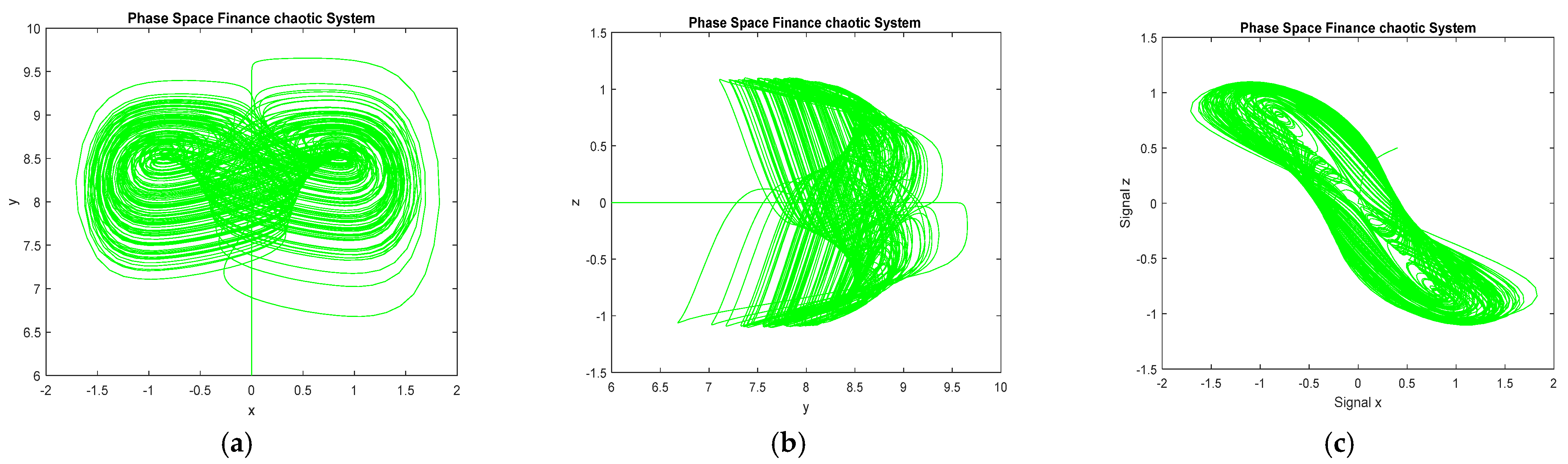
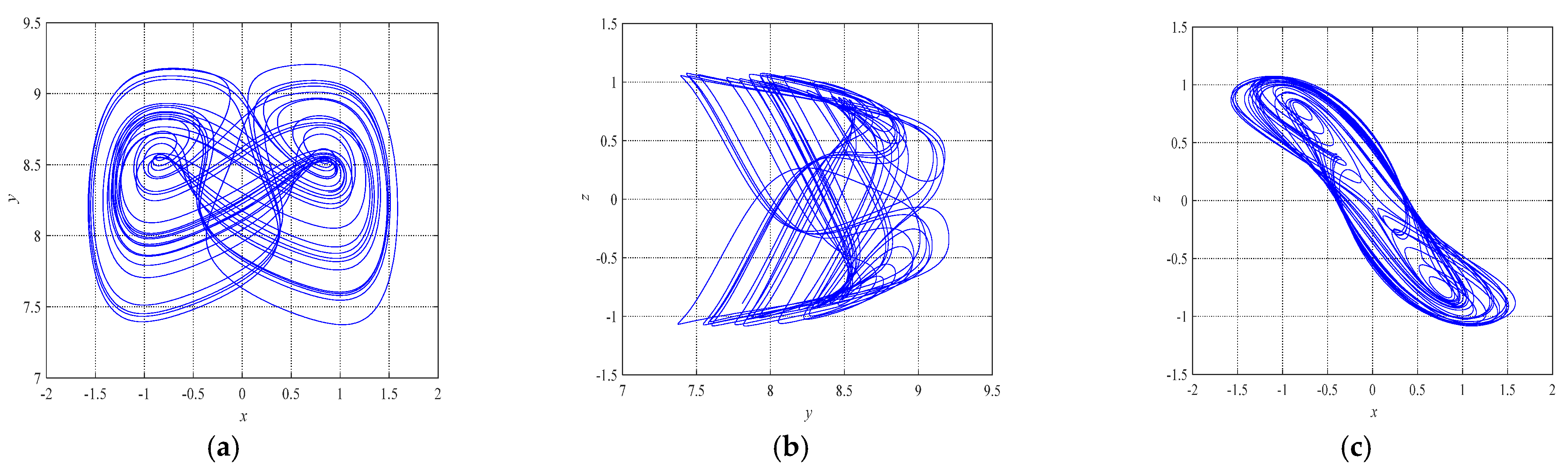
2. Mathematical Models of the Financial Chaotic System

In 2021, Subartini et al. [31] defined a new financial chaotic system as follows:

$$\left\{\begin{array}{l}\dot{x}=z+(y-a)x\\ \dot{y}=1-b(y+x^2)-c{x}^6\\ \dot{z}=-x-z\end{array}\right.$$

(1)

Based on the above system, this study will show that for the following parameter values:

a = 7.6, b = 0.1, c = 0.2

(2)

the system (1) will exhibit a chaotic attractor.

The following initial conditions will be considered in numerical simulations:

x (0) = 0.4, y (0) = 0.2, and z (0) = 0.5

(3)

Using the linear approximation method on the proposed system, the characteristic equation becomes:

$${\mathsf{\lambda }}^3+\underset{C_1}{\underbrace{\left(ab+1\right)}}{\mathsf{\lambda }}^2+\underset{C_2}{\underbrace{\left(a+b+ab+1\right)}}\mathsf{\lambda }+\underset{C_3}{\underbrace{b\left(a+1\right)}}=0$$

(4)

According to Cardano’s Formula [42,43,44], the discriminant $\left(\Delta \right)$ for the above general cubic can be obtained as follows:

$$\Delta =-27C_3{}^2-4C_2{}^3+18 C_1{C}_2{C}_3+C_1{}^2{C}_2{}^2-4C_1{}^3{C}_3$$

(5)

The sign of the discriminant $\left(\Delta \right)$ is very significant in determining the type of root; the potential cases of the roots with the variety discriminant are given by:

$$\mathrm{roots}=\left\{\begin{array}{c}{\mathsf{\lambda }}_1,{\mathsf{\lambda }}_{2,3}=a_i\pm b_{i}i ; if \Delta >0\\ {\mathsf{\lambda }}_1,{\mathsf{\lambda }}_2={\mathsf{\lambda }}_3 ; if \Delta =0\\ {\mathsf{\lambda }}_1\ne {\mathsf{\lambda }}_2\ne {\mathsf{\lambda }}_3 ; if \Delta <0\end{array}\right.$$

(6)

whereas the corresponding roots for each discriminant are given in Formulas (7)–(9), respectively, as:

$${\mathsf{\lambda }}_1=-2\sqrt[3]{\frac{h}{2}}-\frac{C_1}{3}, {\mathsf{\lambda }}_{2,3}=\sqrt[3]{\frac{h}{2}}-\frac{C_1}{3}$$

(7)

$${\mathsf{\lambda }}_{n+1}=\sqrt[6]{16\left(h^2-\Delta \right)}cos\frac{co{s}^{-1}\frac{-h}{\sqrt{h^2-\Delta }}+2\pi n}{3}-\frac{C_1}{3} n=0,1,2.$$

(8)

$$\left\{\begin{array}{l}{\mathsf{\lambda }}_1=\sqrt[3]{\frac{-h-\sqrt{\Delta }}{2}}+\sqrt[3]{\frac{-h+\sqrt{\Delta }}{2}}-\frac{C_1}{3}\\ {\mathsf{\lambda }}_{2,3}=-\frac{1}{2} \left(\sqrt[3]{\frac{-h-\sqrt{\Delta }}{2}}+\sqrt[3]{\frac{-h+\sqrt{\Delta }}{2}}\right)-\frac{C_1}{3 }\pm i\frac{\sqrt{3}}{2}\left(\sqrt[3]{\frac{-h-\sqrt{\Delta }}{2}}-\sqrt[3]{\frac{-h+\sqrt{\Delta }}{2}}\right)\end{array}\right.$$

(9)

in which $h=C_3-\frac{1}{3}{C}_1{C}_2+\frac{2}{27}{C}_1{}^3$.

In order to simplify our results, we chose the parameter to be $\left(a, b,c\right)=\left(7.6, 0.1, 0.2\right)$, and relying on Cardano’s formula, we obtained $\Delta =-88.0026852$ and $h=22.204$, and the values given in

Table 1. The roots of the proposed system obtained via Cardano’s formula.

Iteration	${\mathit{\lambda }}_{\mathbf{1}}$	${\mathit{\lambda }}_{\mathbf{2}}$	${\mathit{\lambda }}_{\mathbf{3}}$
$n=0$	$-0.1$
$n=1$		$-7.4448$
$n=2$			$-1.1552$

are the corresponding roots.

Clearly, from Table 1, the real part of the roots are negative, which means that the new system is stable under the typical parameters. The signal plots of the financial system (1) with initial state Y (0) = (0.4, 0.2, 0.5) and constant parameters (a, b, c) = (7.6, 0.1, 0.2) (chaotic case) are simulated in Figure 1.

The 0-1 test is an effective tool to determine whether the system is in a chaotic state [45]. The regular graph on the p-s plane indicates that the system is in a periodic or quasiperiodic state. Conversely, irregular graphics indicate that the system is in a state of chaos. However, if the system diverges, there will be no graphics on the p-s plane. Figure 2a displays the results of the 0-1 test with irregular graphics. Thus, in this case, the system shows chaotic behavior.

The Poincaré map is used to analyzed the motion characteristics of the multivariable autonomous system [45]. The phase diagram of the Poincaré map well characterizes the reciprocating non-periodic characteristics of chaos. If the Poincaré map is neither a finite set nor a closed curve, then the corresponding system’s motion is in a chaotic motion state. More specifically, if the system does not experience external noise disturbance and there is certain damping, then the Poincaré map will be a point set with a detailed structure. Moreover, if the Poincaré map is a finite set of a point, then the corresponding system motion is periodic. The Poincaré map of system (1) in Figure 2b likewise exhibits chaotic characteristics.

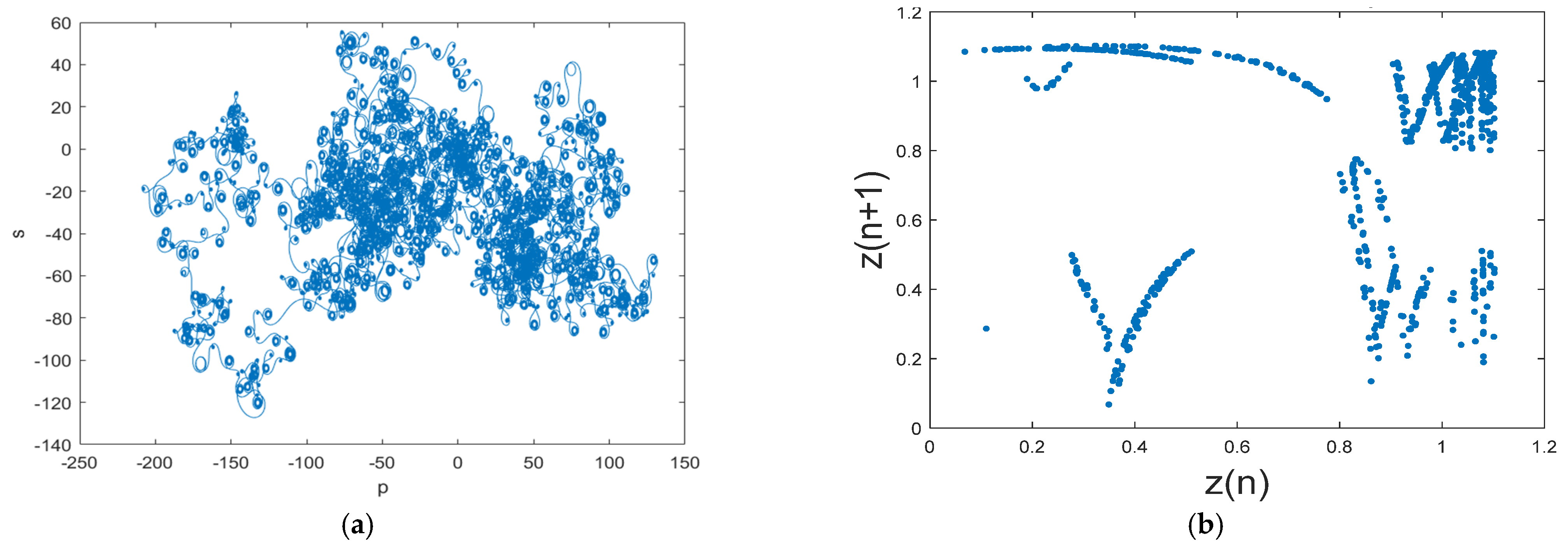
3. Mathematical Model of Fractional-Order Financial Chaotic System

Utilizing the Caputo definition, we have:

$$\begin{array}{l}{D}^{q}f=\frac{1}{\Gamma (n-q)}{\displaystyle \underset{0}{\overset{t}{\int }}{(t-\tau )}^{n-q-1}}{f}^{(n)}(\tau )d\tau \hspace{1em}\hspace{1em}(m-1<q<m)\\ D^{q}f=\frac{d^n}{d{t}^n}f(t)\hspace{1em}\hspace{1em}(q=n)\end{array}$$

(10)

where $\Gamma$ is the gamma function, and m is the lowest integer less than q, with q denoting the order of fractional derivatives. Here,

$$\Gamma (x)={\displaystyle \underset{0}{\overset{\infty }{\int }}{t}^{x-1}{e}^{-t}}dt$$

(11)

The equivalent fractional-order model for system (1) can be mathematically described as follows:

$$\left\{\begin{array}{l}*D_{t_0}^{q}x=z+(y-a)x\\ *D_{t_0}^{q}y=1-b(y+x^2)-c{x}^6\\ *D_{t_0}^{q}z=-x-z\end{array}\right.$$

(12)

with a, b, and c denoting the system parameters, q (0 < q ≤ 1) is the order of the fractional-order differential equation, and the state variables are denoted by x, y, and z.

In Figure 3, we present the phase portrait for financial system (12) of commensurate fractional-order q. Obviously, the fractional-order financial chaotic system (12) can generate chaotic attractors for q = 0.98. Moreover, Figure 4 show the phase portrait’s periodic behavior for the financial system with q = 0.90.

In this work, the special-order q of the fractional financial chaotic system (12) has been used as a parameter to control the bifurcations and develop additional sophisticated dynamics. In this study, the Lyapunov exponent analysis was validated using the Wolf algorithm [46]. We set $\left(a, b,c\right)=\left(7.6, 0.1, 0.2\right)$, with x (0) = 0.4, y (0) = 0.2, and z (0) = 0.5. It is obvious from Figure 5 that the Lyapunov exponent spectrum coincides with the bifurcation diagram. Obviously, the fractional financial system (12) is able to display periodical and chaotic states.

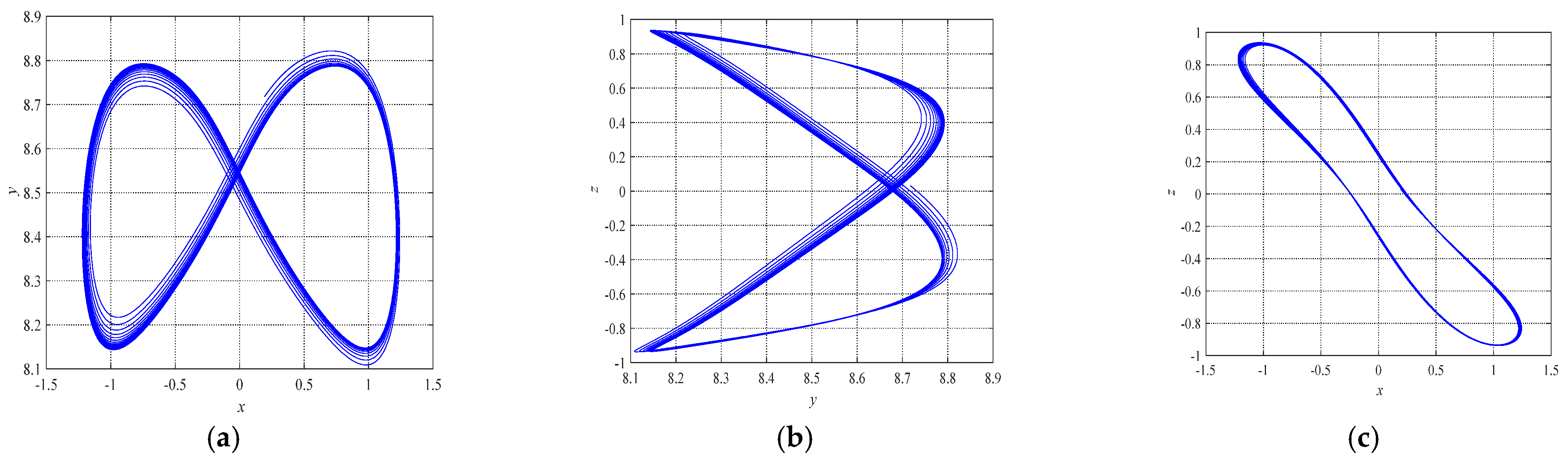
4. Finite-Time Fast Synchronization

In this section, in order to transfer secure communication, we describe chaos control and finite-time fast synchronization.

4.1. Problem Formulation

Consider the new chaotic system (12). In order to achieve synchronization, we divided the new chaos system into two master–slave subsystems.

$$\begin{array}{l}\left.\begin{array}{l}{\dot{x}}_m=z_m+(y_m-a)x_m\\ {\dot{y}}_m=1-b(y_m+x_m^2)-c{x}_m^6\\ {\dot{z}}_m=-x_m-z_m\end{array}\right\}Master \mathrm{subsystem}\\ \\ \left.\begin{array}{l}{\dot{x}}_s=z_s+(y_s-a)x_s+D_1+u_1\\ {\dot{y}}_s=1-b(y_s+x_s^2)-c{x}_s^6+D_2+u_2\\ {\dot{z}}_s=-x_s-z_s+D_3+u_3\end{array}\right\}Slave \mathrm{subsystem}\end{array}$$

(13)

where $\upsilon ={\left[u_1 u_2 u_3\right]}^T$ and $D={\left[D_1 D_2 D_3\right]}^T$ are the control input and bounded uncertainties, respectively.

Assumption 1.

In general,the synchronization of subsystems (13) is as follows:

$$(a_{si}-a_{mi})\left.({\chi }_{si}-{\chi }_{mi})={a^{\prime }}_i{e}_i\right\} \hspace{1em}i=1,2,3$$

(14)

Assumption 2.

We will obtain fast finite-time synchronization between subsystems (13) if

$$\underset{T\to \tau }{\lim }‖e(T)‖, ‖e(T)‖=0 \mathrm{with} T\ge \tau , \mathrm{where} \tau =\tau \left(\mathrm{e}\right(0\left)\right)\text{>}0, \mathrm{e}\left(T\right)={\left[\left(e_i\right)\right]}^T \mathrm{for} \mathrm{i}=1,2,3$$

(15)

Assumption 3.

With ${\chi }_{si}={\chi }_{mi} , i=1,2,3$, the result is:

$$\left.\underset{T\to \infty }{\lim e_i(T)}\right\} i=1,2,3$$

(16)

The fast finite-time synchronization errors, due to Assumptions 1–3 and subsystems (13), are as follows:

$$\begin{array}{l}\left\{\begin{array}{l}{\dot{x}}_s-{\dot{x}}_m=z_s-z_m+(y_s-a_s)x_s-(y_m+a_m)x_m+D_1+B_1{u}_1\\ {\dot{y}}_s-{\dot{y}}_m=1-b_s(y_s+x_s^2)+b_m(y_m+x_m^2)-c{x}_s^6+c{x}_m^6+D_2+B_2{u}_2\\ {\dot{z}}_s-{\dot{z}}_m=-x_s+x_m-z_s+z_m+D_3+B_3{u}_3\end{array}\right.\stackrel{(a_{si}-a_{mi})\left.({\chi }_{si}-{\chi }_{mi})={a^{\prime }}_i{e}_i\right\}}{\to }\\ \\ \left\{\begin{array}{l}\underset{{\dot{e}}_1}{\underbrace{{\dot{x}}_s-{\dot{x}}_m}}=\underset{-a^{\prime }}{\underbrace{(-a_s+a_m)}}\underset{e_1}{\underbrace{(x_s-x_m)}}+\underset{e_3}{\underbrace{(z_s-z_m)}}+\underset{f_1}{\underbrace{(y_s{x}_s-y_m{x}_m)}}+D_1+B_1{u}_1\\ \underset{{\dot{e}}_2}{\underbrace{{\dot{y}}_s-{\dot{y}}_m}}=\underset{-b^{\prime }}{\underbrace{(-b_s+b_m)}}\underset{e_2}{\underbrace{(y_s-y_m)}}+\underset{f_2}{\underbrace{(b_s{x}_s^2-b_m{x}_m^2)+(-c_s{x}_s^6+c_m{x}_m^6)}}+D_2+B_2{u}_2\\ \underset{{\dot{e}}_3}{\underbrace{{\dot{z}}_s-{\dot{z}}_m}}=\underset{-e_1}{\underbrace{(-x_s+x_m)}}+\underset{-e_3}{\underbrace{(-z_s+z_m)}}+D_3+B_3{u}_3\end{array}\right.\end{array}$$

(17)

In the matrix form,

$$\left.\underset{{\dot{e}}_i}{\underbrace{\left[\begin{array}{l}{\dot{e}}_1\\ {\dot{e}}_2\\ {\dot{e}}_3\end{array}\right]}}=\underset{{\chi }_i}{\underbrace{\left[\begin{array}{ccc}-a^{\prime }& 0& 1\\ 0& -\mathrm{b}\text{′}& 0\\ -1& 0& -1\end{array}\right]}}\underset{e_i}{\underbrace{\left[\begin{array}{l}{e}_1\\ e_2\\ e_3\end{array}\right]}}+\underset{f_i}{\underbrace{\left[\begin{array}{l}{f}_1\\ f_2\\ f_3\end{array}\right]}}+\underset{B_i}{\underbrace{\left[B_1 B_2 B_3\right]}}\underset{{\upsilon }_i}{\underbrace{\left[\begin{array}{l}{u}_1\\ u_2\\ u_3\end{array}\right]}}+\underset{{\wp }_i}{\underbrace{\left[{\wp }_1 {\wp }_2 {\wp }_3\right]}}\underset{D_i}{\underbrace{\left[\begin{array}{l}{D}_1\\ D_2\\ D_3\end{array}\right]}}\right\}\hspace{1em}i=1,2,3$$

(18)

where $e_i$ is the error matrix, ${\chi }_i$ is the coefficient matrix, $f_i$ is the nonlinear matrix, ${{\rm B}}_i$ is the controller coefficient, and ${\wp }_i$ is the uncertainty coefficient.

4.2. Adaptive Finite-Time Fast Terminal Sliding Mode Control Approach

According to system (18), the results are as follows:

$$\left.{\dot{e}}_i={\chi }_i{e}_i+f_i+B_i{\upsilon }_i+{\wp }_i{D}_i\right\} \hspace{1em}i=1,2,3$$

(19)

In system (19), the sliding surface is defined as follows:

$$l=\xi e$$

(20)

where $\xi =\left[{\xi }_1 {\xi }_2 {\xi }_3\right]$ is the sliding manifold velocity vector. The fast finite-time sliding surface is given as:

$$\left.\begin{array}{l}\delta =e+\beta {\delta }_1+l^{\raisebox{1ex}{${\mu }_1$}\!\left/ \!\raisebox{-1ex}{${\mu }_2$}\right.}\\ {\dot{\delta }}_1=e+\gamma l^{\raisebox{1ex}{${\eta }_1$}\!\left/ \!\raisebox{-1ex}{${\eta }_2$}\right.}\end{array}\right\}fast finite-time sliding surface$$

(21)

where ${\delta }_1(0)=-{\beta }^{-1}\delta (0),\beta ,\gamma \text{>}0$ are positive constants. $\raisebox{1ex}{${\mu }_1$}\!\left/ \!\raisebox{-1ex}{${\mu }_2$}\right.>\raisebox{1ex}{${\eta }_1$}\!\left/ \!\raisebox{-1ex}{${\eta }_2$}\right.$ are odd integers and $1<\raisebox{1ex}{${\mu }_1$}\!\left/ \!\raisebox{-1ex}{${\mu }_2$}\right.<2.$ With $\delta =0$, we obtain:

$${\dot{\delta }}_1=\left(-\beta {\delta }_1-l^{\raisebox{1ex}{${\mu }_1$}\!\left/ \!\raisebox{-1ex}{${\mu }_2$}\right.}\right)+\gamma {\left(-\beta {\delta }_1-l^{\raisebox{1ex}{${\mu }_1$}\!\left/ \!\raisebox{-1ex}{${\mu }_2$}\right.}\right)}^{\raisebox{1ex}{${\eta }_1$}\!\left/ \!\raisebox{-1ex}{${\eta }_2$}\right.}$$

(22)

We define $\mathrm{{\rm K}}\Gamma =\beta {\delta }_1+l^{\raisebox{1ex}{${\mu }_1$}\!\left/ \!\raisebox{-1ex}{${\mu }_2$}\right.}$. Then, we obtain:

$${\dot{\delta }}_1=-\mathrm{K}\Gamma -{\mathrm{K}}^{\raisebox{1ex}{${\eta }_1$}\!\left/ \!\raisebox{-1ex}{${\eta }_2$}\right.}\gamma {\Gamma }^{\raisebox{1ex}{${\eta }_1$}\!\left/ \!\raisebox{-1ex}{${\eta }_2$}\right.}$$

(23)

Based on Euler–Bernoulli, we have:

$${\delta }_1=-{\mathrm{K}}^{-1}{e}^{-\mathrm{K}{\rm T}}{\left(-\gamma e^{\mathrm{K}\left(1-\raisebox{1ex}{${\eta }_1$}\!\left/ \!\raisebox{-1ex}{${\eta }_2$}\right.\right){\rm T}}+{\beta }^{1-\raisebox{1ex}{${\eta }_1$}\!\left/ \!\raisebox{-1ex}{${\eta }_2$}\right.}{\delta }^{1-\raisebox{1ex}{${\eta }_1$}\!\left/ \!\raisebox{-1ex}{${\eta }_2$}\right.}(0)+\gamma \right)}^{\frac{1}{{}^{1-\raisebox{1ex}{${\eta }_1$}\!\left/ \!\raisebox{-1ex}{${\eta }_2$}\right.}}}$$

(24)

According to Equation (24), finite-time fast convergence is equal to:

$${{\rm T}}_s=\frac{1}{\mathrm{K}\left(1-\raisebox{1ex}{${\eta }_1$}\!\left/ \!\raisebox{-1ex}{${\eta }_2$}\right.\right)}\ln \frac{{\mathrm{K}}^{1-\raisebox{1ex}{${\eta }_1$}\!\left/ \!\raisebox{-1ex}{${\eta }_2$}\right.}{\left|{\delta }_1(0)\right|}^{1-\raisebox{1ex}{${\eta }_1$}\!\left/ \!\raisebox{-1ex}{${\eta }_2$}\right.}+\gamma }{\gamma }=\frac{1}{\mathrm{K}\left(1-\raisebox{1ex}{${\eta }_1$}\!\left/ \!\raisebox{-1ex}{${\eta }_2$}\right.\right)}\ln \frac{{\left|e(0)\right|}^{1-\raisebox{1ex}{${\eta }_1$}\!\left/ \!\raisebox{-1ex}{${\eta }_2$}\right.}+\gamma }{\gamma }$$

(25)

Theorem 1.

Consider the nonlinear system (19). With sliding surface (21), we define the control input as follows:

$$\dot{\upsilon }=B_i^{-1}\left\{\left({\chi }_i{e}_i+f_i-sign({\delta }_i)‖{\wp }_i‖D_{mi}\right)+\left(-\beta e_i-\beta \gamma e_i^{\raisebox{1ex}{${\eta }_1$}\!\left/ \!\raisebox{-1ex}{${\eta }_2$}\right.}-\frac{{\mu }_1}{{\mu }_2}{l}^{1-\raisebox{1ex}{${\mu }_1$}\!\left/ \!\raisebox{-1ex}{${\mu }_2$}\right.}{e}_i\right)-\lambda \frac{{\delta }_i}{‖{\delta }_i‖}\right\}$$

(26)

where $D_{mi}, \mathrm{i}=1,2,3$ are the upper bounds of uncertainty and $\lambda$ is the positive definite (pd) matrix and it is constant. By properly selecting the parameters defined in the newly designed controller, we will achieve fast finite-time convergence.

Proof. 

To validate the controller, let the function of the Lyapunov candidate be defined as follows:

$$\nu (t)=\frac{({\delta }_i{}^T{\delta }_i)}{2}$$

(27)

The sliding surface $\delta$ derivative is obtained as follows:

$${\dot{\delta }}_i={\dot{e}}_i+\beta {\dot{\delta }}_1+\frac{{\mu }_1}{{\mu }_2}{\left|l\right|}^{{}^{\raisebox{1ex}{${\mu }_1$}\!\left/ \!\raisebox{-1ex}{${\mu }_2$}\right.-1}}\dot{l}$$

(28)

By placing (19) in (28), the result is:

$${\dot{\delta }}_i=\left({\chi }_i{e}_i+f_i+B_i{\upsilon }_i+{\wp }_i{D}_i\right)+\beta \left(e+\gamma e^{\raisebox{1ex}{${\eta }_1$}\!\left/ \!\raisebox{-1ex}{${\eta }_2$}\right.}\right)+\frac{{\mu }_1}{{\mu }_2}{\left|e\right|}^{{}^{{}^{\raisebox{1ex}{${\mu }_1$}\!\left/ \!\raisebox{-1ex}{${\mu }_2$}\right.-1}}}e$$

(29)

Substituting the new controller (26) into the derivative of the Lyapunov candidate function (27), the result is:

$$\begin{array}{ll}\dot{\nu }(t)& ={\delta }_i{}^{{\rm T}}\left({\wp }_i{D}_i\right.-‖{\wp }_i‖sign({\delta }_i)D_{mi}-\beta \left(e+\gamma e^{\raisebox{1ex}{${\eta }_1$}\!\left/ \!\raisebox{-1ex}{${\eta }_2$}\right.}\right)-\frac{{\mu }_1}{{\mu }_2}{l}^{1-\raisebox{1ex}{${\mu }_1$}\!\left/ \!\raisebox{-1ex}{${\mu }_2$}\right.}e\\ & -\lambda \frac{{\delta }_i}{‖{\delta }_i‖}+\beta {\dot{\delta }}_1+\frac{{\mu }_1}{{\mu }_2}{\left|l\right|}^{{}^{{}^{\raisebox{1ex}{${\mu }_1$}\!\left/ \!\raisebox{-1ex}{${\mu }_2$}\right.-1}}}\left.\dot{l}\right)\\ & ={\delta }_i{}^{{\rm T}}{\wp }_i{D}_i-{\delta }_i{}^{{\rm T}}‖{\delta }_i‖sign({\delta }_i)D_{mi}-{\delta }_i{}^{{\rm T}}\lambda \frac{{\delta }_i}{‖{\delta }_i‖}\end{array}$$

(30)

We obtain:

$$\begin{array}{l}\left({\delta }_i{}^{{\rm T}}{\wp }_i{D}_i-‖{\delta }_i‖sign({\delta }_i)D_{mi}\right)\\ ={\displaystyle \sum _{i=1}^3{\delta }_i}{\wp }_i{D}_i-{\displaystyle \sum _{i=1}^3\left|{\delta }_i\right|}{\wp }_{i}sign({\delta }_i)D_{mi}\\ \le {\displaystyle \sum _{i=1}^3\left|{\delta }_i\right|}\left|{\wp }_i{D}_i\right|-{\displaystyle \sum _{i=1}^3\left|{\delta }_i\right|}\left|{\wp }_i\right|D_{im}\le 0\end{array}$$

(31)

By extending Equation (30) and according to Equation (31), the results are:

$$\begin{array}{ll}\dot{\nu }(t)& \le -{\delta }_i^{{\rm T}}\lambda \frac{{\delta }_i}{‖{\delta }_i‖}\\ & \le -{\sigma }_{\min }(\lambda )\frac{{‖{\delta }_i‖}^2}{‖{\delta }_i‖}\\ & \le -\sqrt{2}{\sigma }_{\min }(\lambda ){\nu }^{0.5}(t)\end{array}$$

(32)

Thus, it can be concluded that the sliding surface converges to the origin within a fast finite time. Convergence time is equal to:

$${{\rm T}}_s\le \frac{{\nu }^{0.5}\left({\delta }_i(t_0)\right)}{\raisebox{1ex}{$1$}\!\left/ \!\raisebox{-1ex}{$\sqrt{2}{\sigma }_{\min }(\lambda )$}\right.}=\frac{‖{\delta }_i(t_0)‖}{{\sigma }_{\min }(\lambda )}$$

(33)

The proof is complete. $\square$

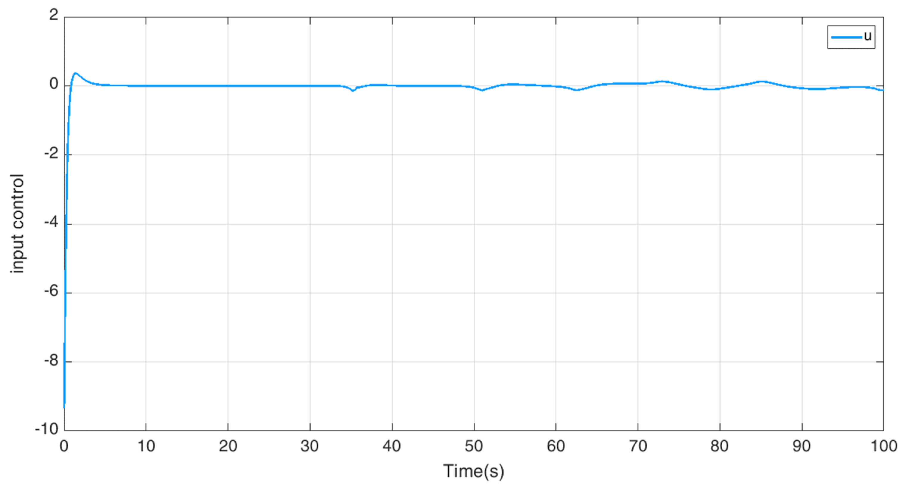
4.3. Simulation Results of Adaptive Finite-Time Fast Terminal Sliding Mode Control

In this section, using MATLAB software, a simulation is described between two new nonlinear systems (13), with the new control system being defined in (26). By synchronizing these two systems, we achieve the goals of secure communication in a fast, finite timeframe.

The initial conditions and parameters of systems (13) are as follows:

$$\begin{array}{l}\left.\begin{array}{l}{a}_m=7.6, b_m=0.1, c_m=0.2\\ x_m(0)=0.4, y_m(0)=0.2, z_m(0)=0.5\end{array}\right\}master values\\ \\ \left.\begin{array}{l}{a}_s=7.2, b_s=0.16, c_s=0.18\\ x_s(0)=-1.5, y_s(0)=-1.33, z_s(0)=-1.78\end{array}\right\}slave values\end{array}$$

(34)

The controller parameters’ numerical values are shown in

Table 2. The controller values.

Parameter	Value
$\beta$	0.24
$\gamma$	0.036
${\mu }_1$	37
${\mu }_2$	11
${\eta }_1$	21
${\eta }_2$	9
$\lambda$	diag(0.5   1   1.5)
$\mathrm{K}$	diag(0.57   0.29   0.06)
${\wp }_i$	[3.2   0.5   4.8]
${{\rm B}}_i$	[1   1   1]

.

The disturbances are given as:

$$D_i=\left[\begin{array}{l}0.3+0.6\sin (\varpi t)\\ 0.8-0.7\cos (2\varpi t)\\ 0.4-0.9\sin (1.2\varpi t)\end{array}\right]$$

(35)

Under the new controller (26), the complete synchronization and error synchronization of the nonlinear master–slave systems (13) are as presented in Figure 6, Figure 7 and Figure 8. The controller input is shown in Figure 9.

As it was observed, synchronization between the master–slave subsystems is performed in a finite timeframe, and synchronization errors converge with very little error near the origin. Thus, we will achieve fast secure communication.

5. Conclusions

In this study, we have presented the complex behaviors of the financial chaotic system in fractional order with two quadratic nonlinearities and a sextic nonlinearity. We validated the existence of chaos via the phase portraits, 0-1 test, Poincaré map, bifurcation diagram, and Lyapunov exponent. The analysis showed that the financial risk chaotic system of fractional order is able to exhibit chaotic behavior and periodical behavior. Finally, an illustrative example was given, and the terminal adaptive finite-time SMC technique was analyzed. The demonstrative examples were discussed to illustrate the efficacy and applicability of the new finite-time control strategy.

References

1. Zhuo, P.J.; Zhang, Z.X.; Gou, X.F. Chaotic motion of a magnet levitated over a superconductor. IEEE Trans. Appl. Supercond. 2016, 26, 1–6. [Google Scholar] [CrossRef]
2. Abro, K.A. Numerical study and chaotic oscillations for aerodynamic model of wind turbine via fractal and fractional differential operators. Numer. Methods Partial. Differ. Equ. 2022, 38, 1180–1194. [Google Scholar] [CrossRef]
3. Pappu, C.S.; Carroll, T.L.; Flores, B.C. Simultaneous radar-communication systems using controlled chaos-based frequency modulated waveforms. IEEE Access 2020, 8, 48361–48375. [Google Scholar] [CrossRef]
4. Sambas, A.; Vaidyanathan, S.; Zhang, X.; Koyuncu, I.; Bonny, T.; Tuna, M.; Alcin, M.; Zhang, S.; Sulaiman, I.M.; Awwal, A.M.; et al. A Novel 3D Chaotic System with Line Equilibrium: Multistability, Integral Sliding Mode Control, Electronic Circuit, FPGA and its Image Encryption. IEEE Access 2022, 10, 68057–68074. [Google Scholar] [CrossRef]
5. Mou, J.; Sun, K.; Ruan, J.; He, S. A nonlinear circuit with two memcapacitors. Nonlinear Dyn. 2016, 86, 1735–1744. [Google Scholar] [CrossRef]
6. Naik, R.D.; Singru, P.M. Resonance, stability and chaotic vibration of a quarter-car vehicle model with time-delay feedback. Commun. Nonlinear Sci. Numer. Simul. 2011, 16, 3397–3410. [Google Scholar] [CrossRef]
7. Fakhraei, J.; Khanlo, H.M.; Ghayour, M. Chaotic behaviors of a ground vehicle oscillating system with passengers. Sci. Iranica. Trans. B Mech. Eng. 2017, 24, 1051. [Google Scholar] [CrossRef] [Green Version]
8. Lim, T.S.; Lu, Y.; Nolen, J.H. Quantitative propagation of chaos in a bimolecular chemical reaction-diffusion model. SIAM J. Math. Anal. 2020, 52, 2098–2133. [Google Scholar] [CrossRef]
9. Li, S.; He, Y.; Cao, H. Necessary conditions for complete synchronization of a coupled chaotic Aihara neuron network with electrical synapses. Int. J. Bifurc. Chaos 2019, 29, 1950063. [Google Scholar] [CrossRef]
10. Sambas, A.; Vaidyanathan, S.; Bonny, T.; Zhang, S.; Hidayat, Y.; Gundara, G.; Mamat, M. Mathematical model and FPGA realization of a multi-stable chaotic dynamical system with a closed butterfly-like curve of equilibrium points. Appl. Sci. 2021, 11, 788. [Google Scholar] [CrossRef]
11. Nakamura, Y.; Sekiguchi, A. The chaotic mobile robot. IEEE Trans. Robot. Autom. 2001, 17, 898–904. [Google Scholar] [CrossRef]
12. Atangana, A.; Bonyah, E.; Elsadany, A.A. A fractional order optimal 4D chaotic financial model with Mittag-Leffler law. Chin. J. Phys. 2020, 65, 38–53. [Google Scholar] [CrossRef]
13. Bekiros, S.; Jahanshahi, H.; Munoz-Pacheco, J.M. A new buffering theory of social support and psychological stress. PLoS one 2022, 17, e0275364. [Google Scholar] [CrossRef] [PubMed]
14. Fanti, L.; Manfredi, P. Chaotic business cycles and fiscal policy: An IS-LM model with distributed tax collection lags. Chaos Solitons Fractals 2007, 32, 736–744. [Google Scholar] [CrossRef]
15. Orlando, G. A discrete mathematical model for chaotic dynamics in economics: Kaldor’s model on business cycle. Math. Comput. Simul. 2016, 125, 83–98. [Google Scholar] [CrossRef]
16. Barnett, W.A.; Bella, G.; Ghosh, T.; Mattana, P.; Venturi, B. Shilnikov chaos, low interest rates, and New Keynesian macroeconomics. J. Econ. Dyn. Control. 2022, 134, 104291. [Google Scholar] [CrossRef]
17. Kyrtsou, C.; Labys, W.C. Evidence for chaotic dependence between US inflation and commodity prices. J. Macroecon. 2006, 28, 256–266. [Google Scholar] [CrossRef]
18. Sukono; Sambas, A.; He, S.; Liu, H.; Vaidyanathan, S.; Hidayat, Y.; Saputra, J. Dynamical analysis and adaptive fuzzy control for the fractional-order financial risk chaotic system. Adv. Differ. Equ. 2020, 2020, 674. [Google Scholar] [CrossRef]
19. Munoz-Pacheco, J.M.; Zambrano-Serrano, E.; Volos, C.; Tacha, O.I.; Stouboulos, I.N.; Pham, V.T. A fractional order chaotic system with a 3D grid of variable attractors. Chaos Solitons Fractals 2018, 113, 69–78. [Google Scholar] [CrossRef]
20. Wang, Y.L.; Jahanshahi, H.; Bekiros, S.; Bezzina, F.; Chu, Y.M.; Aly, A.A. Deep recurrent neural networks with finite-time terminal sliding mode control for a chaotic fractional-order financial system with market confidence. Chaos Solitons Fractals 2021, 146, 110881. [Google Scholar] [CrossRef]
21. Chen, W.C. Nonlinear dynamics and chaos in a fractional-order financial system. Chaos Solitons Fractals 2008, 36, 1305–1314. [Google Scholar] [CrossRef]
22. Li, H.L.; Hu, C.; Zhang, L.; Jiang, H.; Cao, J. Complete and finite-time synchronization of fractional-order fuzzy neural networks via nonlinear feedback control. Fuzzy Sets Syst. 2022, 443, 50–69. [Google Scholar] [CrossRef]
23. Li, H.L.; Jiang, H.; Cao, J. Global synchronization of fractional-order quater-nion-valued neural networks with leakage and discrete delays. Neurocomputing 2020, 385, 211–219. [Google Scholar] [CrossRef]
24. Wang, S.; He, S.; Yousefpour, A.; Jahanshahi, H.; Repnik, R.; Perc, M. Chaos and complexity in a fractional-order financial system with time delays. Chaos Solitons Fractals 2020, 131, 109521. [Google Scholar] [CrossRef]
25. Pan, I.; Korre, A.; Das, S.; Durucan, S. Chaos suppression in a fractional order financial system using intelligent regrouping PSO based fractional fuzzy control policy in the presence of fractional Gaussian noise. Nonlinear Dyn. 2012, 70, 2445–2461. [Google Scholar] [CrossRef]
26. Wang, Z.; Huang, X.; Zhao, Z. Synchronization of nonidentical chaotic fractional-order systems with different orders of fractional derivatives. Nonlinear Dyn. 2012, 69, 999–1007. [Google Scholar] [CrossRef]
27. Hajipour, A.; Tavakoli, H. Dynamic analysis and adaptive sliding mode controller for a chaotic fractional incommensurate order financial system. Int. J. Bifurc. Chaos 2017, 27, 1750198. [Google Scholar] [CrossRef]
28. Yousri, D.; Mirjalili, S. Fractional-order cuckoo search algorithm for parameter identification of the fractional-order chaotic, chaotic with noise and hyper-chaotic financial systems. Eng. Appl. Artif. Intell. 2020, 92, 103662. [Google Scholar] [CrossRef]
29. Cao, Y. Chaotic synchronization based on fractional order calculus financial system. Chaos Solitons Fractals 2020, 130, 109410. [Google Scholar] [CrossRef]
30. Wang, B.; Liu, J.; Alassafi, M.O.; Alsaadi, F.E.; Jahanshahi, H.; Bekiros, S. Intelligent parameter identification and prediction of variable time fractional derivative and application in a symmetric chaotic financial system. Chaos Solitons Fractals 2022, 154, 111590. [Google Scholar] [CrossRef]
31. Subartini, B.; Vaidyanathan, S.; Sambas, A.; Zhang, S. Multistability in the Finance Chaotic System, Its Bifurcation Analysis and Global Chaos Synchronization via Integral Sliding Mode Control. IAENG Int. J. Appl. Math. 2021, 51, 995–1002. [Google Scholar]
32. Xu, X.; Lee, S.D.; Kim, H.S.; You, S.S. Management and optimisation of chaotic supply chain system using adaptive sliding mode control algorithm. Int. J. Prod. Res. 2021, 59, 2571–2587. [Google Scholar] [CrossRef]
33. Yin, C.; Dadras, S.; Zhong, S.M.; Chen, Y. Control of a novel class of fractional-order chaotic systems via adaptive sliding mode control approach. Appl. Math. Model. 2013, 37, 2469–2483. [Google Scholar] [CrossRef]
34. Yan, J.J.; Hung, M.L.; Liao, T.L. Adaptive sliding mode control for synchronization of chaotic gyros with fully unknown parameters. J. Sound Vib. 2006, 298, 298–306. [Google Scholar] [CrossRef]
35. Ghamati, M.; Balochian, S. Design of adaptive sliding mode control for synchronization Genesio–Tesi chaotic system. Chaos Solitons Fractals 2015, 75, 111–117. [Google Scholar] [CrossRef]
36. Mohadeszadeh, M.; Delavari, H. Synchronization of fractional-order hyperchaotic systems based on a new adaptive sliding mode control. Int. J. Dyn. Control. 2017, 5, 124–134. [Google Scholar] [CrossRef]
37. Li, W.L.; Chang, K.M. Robust synchronization of drive–response chaotic systems via adaptive sliding mode control. Chaos Solitons Fractals 2009, 39, 2086–2092. [Google Scholar] [CrossRef]
38. Min, F.; Li, C.; Zhang, L.; Li, C. Initial value-related dynamical analysis of the memristor-based system with reduced dimensions and its chaotic synchronization via adaptive sliding mode control method. Chin. J. Phys. 2019, 58, 117–131. [Google Scholar] [CrossRef]
39. Maeng, G.; Choi, H.H. Adaptive sliding mode control of a chaotic non-smooth-air-gap permanent magnet synchronous motor with uncertainties. Nonlinear Dyn. 2013, 74, 571–580. [Google Scholar] [CrossRef]
40. Khan, A.; Singh, S. Generalization of combination-combination synchronization of n-dimensional time-delay chaotic system via robust adaptive sliding mode control. Math. Methods Appl. Sci. 2018, 41, 3356–3369. [Google Scholar] [CrossRef]
41. Shang, Z.; Yu, Y.; Li, Y. Adaptive sliding mode control of chaotic oscilla-tion in power system based on relay characteristic function. In Proceedings of the 2020 IEEE/IAS Industrial and Commercial Power System Asia (I&CPS Asia), Weihai, China, 13–15 July 2020; pp. 1012–1016. [Google Scholar]
42. Shukla, V.K.; Vishal, K.; Srivastava, M.; Singh, P.; Singh, H. Multi-switching compound synchronization of different chaotic systems with external disturbances and parametric uncertainties via two approaches. Int. J. Appl. Comput. Math. 2022, 8, 1–22. [Google Scholar] [CrossRef]
43. Aqeel, M.; Ahmad, S.; Azam, A.; Ahmed, F. Dynamical and fractal properties in periodically forced stretch-twist-fold (STF) flow. Eur. Phys. J. Plus 2007, 132, 1–13. [Google Scholar] [CrossRef]
44. Al-Azzawi, S.F. Stability and bifurcation of pan chaotic system by using Routh–Hurwitz and Gardan methods. Appl. Math. Comput. 2012, 219, 1144–1152. [Google Scholar] [CrossRef]
45. Sun, K. Chaotic Secure Communication: Principles and Technologies. Tsinghua University Press and Walter de Gruyter GmbH: Beijing, China, 2016; pp. 119–135. [Google Scholar]
46. Wolf, A.; Swift, J.B.; Swinney, H.L.; Vastano, J.A. Determining Lyapunov exponents from a time series. Phys. D Nonlinear Phenom. 1985, 16, 285–317. [Google Scholar] [CrossRef]
Figure 1. Output MATLAB simulation of the financial chaotic system (1) with Y (0) = (0.4, 0.2, 0.5) and (a, b, c) = (7.6, 0.1, 0.2): (a) x-y plane, (b) y-z plane, and (c) x-z plane.
Mathematics 11 00100 g001
Figure 2. Output MATLAB simulation of the financial chaotic system (1) with Y (0) = (0.4, 0.2, 0.5) and (a, b, c) = (7.6, 0.1, 0.2): (a) x-y plane, and (b) Poincaré section of the financial chaotic system (1).
Mathematics 11 00100 g002
Figure 3. Phase diagrams for q = 0.98, a ,   b , c = 7.6 ,   0.1 ,   0.2 with x (0) = 0.4, y (0) = 0.2, z (0) = 0.5: (a) x-y plane, (b) y-z plane, and (c) x-z plane.
Mathematics 11 00100 g003
Figure 4. Phase diagrams for q = 0.90, a ,   b , c = 7.6 ,   0.1 ,   0.2 with x (0) = 0.4, y (0) = 0.2, z (0) = 0.5: (a) x-y plane, (b) y-z plane, and (c) x-z plane.
Mathematics 11 00100 g004
Figure 5. MATLAB simulation for financial fractional-order chaotic system: (a) Lyapuov exponent for q [0.9 1] and (b) bifurcation diagram for q [0.9 1].
Mathematics 11 00100 g005
Figure 6. The master–slave synchronization of the first state.
Mathematics 11 00100 g006
Figure 7. The master–slave synchronization of the second state.
Mathematics 11 00100 g007
Figure 8. The master–slave synchronization of the third state.
Mathematics 11 00100 g008
Figure 9. Input control.
Mathematics 11 00100 g009