Several Control Problems of a Class of Complex Nonlinear Systems Based on UDE

Abstract

This paper mainly studies several control problems of a complex 4D chaotic system. Firstly, the real part and imaginary part of the complex 4D chaotic system are separated, and the system is equivalent to a six-dimensional continuous autonomous real chaotic system. Then, the stabilization, synchronization, and anti-synchronization of the complex four-dimensional chaotic system are realized by using the control method of the combination of dynamic feedback gain control and UDE control, and the corresponding physical controllers are designed respectively. Finally, the correctness and effectiveness of the theoretical results are verified by numerical simulation.

1. Introduction

Since Lorenz first discovered the chaotic system in 1963, a popular direction with great research value is the chaotic system and its phenomenon [1]. Recently, studying chaotic systems with unique properties has attracted lots of attention. Chaotic flows with a specific solution and chaotic flows with imprisoned strange attractors have been investigated [2,3,4]. From a numerical viewpoint, many promotions have been done with the help of some pioneer researchers [5]. The complex chaotic system whose state variables belong to the complex space is another important type of chaotic dynamic system [6,7,8]. It has been extensively studied in theorem and application and has become a hot topic in recent years. Especially since the complex chaotic system is composed of real numbers and imaginary numbers, it has a better encryption effect than the real chaotic system [9,10]. Since the dynamic behavior of complex chaotic systems is more complicated than real chaotic systems, it is very difficult to study the control problems of such systems [11].

Although the traditional linear feedback controller has a simple structure and is easy to implement physically, it also has the problem of relying too much on the value of the control feedback gain, which greatly limits the freedom of setting the initial value of the system [12,13,14]. At present, most researchers adopt the following method. Firstly, by separating the real and imaginary parts of the complex state variable, the complex chaotic system is transformed into its equivalent real chaotic system, then the corresponding controller is designed for the controlled real chaotic system; finally, according to the corresponding relationship between the complex chaotic system and the real chaotic system, the corresponding controller of the complex chaotic system is obtained to realize the control problem of this kind of complex system [15,16,17]. However, this method also has some problems. On the one hand, the first step lacks a systematic method; that is, for a specific complex chaotic system, how to find a systematic method to transform the complex chaotic system into its equivalent real chaotic system [18,19]. Not only has important theoretical significance, but also has a wide range of application values [20,21,22]; on the other hand, most of the controllers designed by previous researchers are mostly complex [23,24]; therefore, they are difficult to apply in practical situations [23,25,26]. Regarding the control problem of solving nonlinear systems, there are also controllers to choose from in physics, and the uncertainty and disturbance estimation controller is one of them. The core part of the UDE controller is composed of several filters with sufficiently large bandwidth. The basic principle of solving the external disturbance and uncertainty of the system is to use filters of appropriate structure to accurately estimate the internal model of a given nonlinear system. Uncertainty and external disturbances, and then filter them out, so that the filtered system reaches a stable state again [27,28,29].

Motivated by the above conclusions, we study the existence of anti-synchronization problems in a class of complex nonlinear systems by the dynamic control method and UDE control method. The main contributions of this paper are listed as follows:

(a)

A method of transforming the hyper-chaotic model with cubic nonlinearity and complex variables into an equivalent real chaotic system is proposed.

(b)

A previously known dynamic gain feedback controller is used to realize the stabilization control, synchronization control, and anti-synchronization control of the nominal system.

(c)

Combining the dynamic gain feedback control method and the uncertainty and disturbance estimation control method, a combined controller is proposed to solve the stabilization, complete synchronization, and anti-synchronization problems of a class of complex variable chaotic systems with model uncertainty and external disturbances. Finally, a simulation example is given to verify the feasibility and effectiveness of the designed controller.

2. Preliminary

Consider the following controlled chaotic system with model uncertainty and external disturbance:

$$\dot{g}=f(g)+Bu+u_d$$

(1)

$$u_d=\Delta f(g)+d(t)$$

(2)

where $g\in {ℝ}^n$ is the state, $(f(g),B)$ is controllable, $B\in {ℝ}^{n\times r}$ is a constant matrix, $r\ge 1$, $u\in {ℝ}^r$ is the designed controller, $\Delta f(g)$ is the uncertainty of the model, and $d(t)$ is an external disturbance.

Consider the following controlled chaotic system:

$$\dot{g}=f(g)+Bu$$

(3)

where $g\in {ℝ}^n$ is the state, $(f(g),B)$ is controllable, $B\in {ℝ}^{n\times r}$ is a constant matrix, $r\ge 1$, and $u\in {ℝ}^r$ is the designed controller. If $\underset{t\to \infty }{\lim }‖g(t)‖=0$, it is said that the system has achieved stabilization.

For this system, the controller $u$ has the following form:

$$u=u_s+u_{ude}$$

(4)

where

$$u_s=K(t)g(t)=k(t)B^{T}g(t)$$

(5)

$$u_{ude}=B^{+}[(F(g)-\dot{g})\ast \frac{g_f(t)}{1-g_f(t)}]$$

(6)

Consider the following controlled chaotic system with model uncertainty and external disturbance:

$$\dot{g}=f(g)+\Delta f(g)+d(t)$$

(7)

where $g\in {ℝ}^n$ is the state, $f(g)=[f_1(g),f_2(g),\dots ,f_n(g)]$ is continuous vector function, $\Delta f(g)$ is the uncertainty of the model, and $d(t)$ is an external disturbance.

$$\dot{h}=f(h)+Bu$$

(8)

where $h\in {ℝ}^n$ is the state, $f(h)=[f_1(h),f_2(h),\dots ,f_n(h)]$ is the continuous vector function, $B\in {ℝ}^{n\times r}$ is the real constant matrix and $r\ge 1$, $u$ is given in Equation (4).

Let $e=h-\alpha g$, then the error system can be expressed as:

$$\begin{array}{l}\dot{e}=f(h)-\alpha f(g)+B{u}_s+B{u}_{ude}-\alpha u_d\\ =G(g,e)+B{u}_{ude}-\alpha u_d\end{array}$$

(9)

where $e\in {ℝ}^n$ is the state, $B$ is given in Equation (3)

$$\alpha =\left(\begin{array}{ccc}{\alpha }_1& \dots & 0\\ ⋮& \ddots & ⋮\\ 0& \cdots & {\alpha }_n\end{array}\right)$$

where $\left|{\alpha }_i\right|=1, i\in \Lambda =\{1,2,\dots ,n\}$.

Consider the error system (9), if $\alpha$ is a unit matrix, ${\alpha }_i=1$, $i\in \Lambda$, system (9) can be rewritten as:

$$e=f(h)-f(g)+Bu-u_d$$

(10)

If $\underset{t\to \infty }{\lim }‖e(t)‖=0$, it indicates that master system (7) and slave system (8) have achieved complete synchronization.

Consider the error system (9), if $\alpha$ is a negative unit matrix, ${\alpha }_i=-1$, $i\in \Lambda$, system (9) can be rewritten as:

$$e=f(h)+f(g)+Bu+u_d$$

(11)

If $\underset{t\to \infty }{\lim }‖e(t)‖=0$, it indicates that master system (7) and slave system (8) have achieved anti-synchronization.

Lemma 1.

Consider the following controlled chaotic system

$$\dot{p}=h(p)+bu$$

(12)

where$p\in {ℝ}^n$is the state,$b\in {ℝ}^{n\times r}$is a constant matrix,$r\ge 1$and$u\in {ℝ}^r$is the designed controller. If$(h(p),b)$is controllable, the designed dynamic gain feedback controller is:

$$u=Kp$$

(13)

where$K=k(t)b^T$, and the update rate of dynamic gain is:

$$\dot{k}(t)=-{‖p(t)‖}^2$$

(14)

Lemma 2.

Consider the following controlled chaotic system with model uncertainty and external disturbance:

$$\dot{g}=f(g)+\Delta f(g)+d(t)$$

(15)

where$g\in {ℝ}^n$is the state,$\Delta f(g)$is the uncertainty of the model,$d(t)$is an external disturbance.

$$\dot{k}(t)=-{‖p(t)‖}^2$$

(16)

$${\widehat{u}}_d=(\dot{g}-F(g)-B{u}_{ude})*g_f(t)$$

(17)

The designed controller has the following forms:

$$u=u_{ude}+u_s$$

(18)

where

$$\begin{array}{l}{u}_s=K(t)g(t)=k(t)B^{T}g(t)\\ u_{ude}=B^{+}[{\ell }^{-1}[\frac{G_f(t)}{1-G_f(t)}]*F(g)-{\ell }^{-1}[\frac{G_f(t)}{1-G_f(t)}]*g]\end{array}$$

(19)

$F(g)=f(g)+u_s=f(g)+k(t)B^{T}g(t)$,$B^{+}={(B^{T}B)}^{-1}{B}^T$,$G_f(s)=\ell [g_f(t)]$,$\ell$represents Laplace transform,${\ell }^{-1}$represents inverse Laplace transform, * represents convolution, and the update rate of dynamic gain

$$\dot{k}(t)=-{‖p(t)‖}^2$$

(20)

Remark 1.

According to the existing result in Equation (19), the following two kinds of filters, which can deal with various common model uncertainties and external disturbances

• first-order low-pass filter:

  $$G_f(s)=\frac{1}{1+\tau s},\tau =0.001$$

  (21)
• secondary filter:

  $$G_f(s)=\frac{a_{1}s+a_2-{\omega }_0^2}{s^2+a_{1}s+a_2}$$

  (22)

  where${\omega }_0=4\pi ,a_1=10{\omega }_0,a_2=100{\omega }_0^2$.

3. Problem Formulation

According to Ref. [19], the 4D hyper-chaotic system is given as:

$$\left\{\begin{array}{l}\dot{m}=20(m-n)+npq\\ \dot{n}=3(m+n)-mpq\\ \dot{p}=\frac{1}{2}(\overline{m}n+m\overline{n})q-p\\ \dot{q}=\frac{1}{2}(\overline{m}n+m\overline{n})p-2q\end{array}\right.$$

(23)

where $m,n$ are complex variables and $p,q$ are real variables.

Let $m=g_1+i{g}_2$ and $n=g_3+i{g}_4$ be complex functions, $p=g_5$ and $q=g_6$ be real variables. Dots represent derivatives with respect to time and $i=\sqrt{-1}$.

Convert system (23) to the following six-dimensional real system

$$\left\{\begin{array}{l}{\dot{g}}_1=20(g_3-g_1)+g_3{g}_5{g}_6\\ {\dot{g}}_2=20(g_4-g_2)+g_4{g}_5{g}_6\\ {\dot{g}}_3=3(g_1+g_3)-g_1{g}_5{g}_6\\ {\dot{g}}_4=3(g_2+g_4)-g_2{g}_5{g}_6\\ {\dot{g}}_5=(g_1{g}_3+g_2{g}_4)g_6-g_5\\ {\dot{g}}_6=(g_1{g}_3+g_2{g}_4)g_5-2g_6\end{array}\right.$$

(24)

where $g\in {ℝ}^6$ is the state.

This paper investigates the stabilization, complete synchronization, and anti-synchronization problems of system (24) and presents some new results.

4. Main Result

In this section, we investigate the stabilization, synchronization, and anti-synchronization of complex 4D systems by the control method of the combination of dynamic feedback gain control and UDE control.

4.1. Stabilization of Systems

Consider the following controlled complex 4D hyper-chaotic system with model uncertainty and external disturbance:

$$\dot{g}=f(g)+Bu+u_d$$

(25)

$$u_d=\Delta f(g)+d(t)$$

(26)

where $g\in {ℝ}^6$ is the state of the system, $f(g)$ is given in Equation (24), and $u$ is the controller to be designed.

$$f(g)=\left(\begin{array}{l}{f}_1(g)\\ f_2(g)\\ f_3(g)\\ f_4(g)\\ f_5(g)\\ f_6(g)\end{array}\right)=\left(\begin{array}{l}20(g_3-g_1)+g_3{g}_5{g}_6\\ 20(g_4-g_2)+g_4{g}_5{g}_6\\ 3(g_1+g_3)-g_1{g}_5{g}_6\\ 3(g_2+g_4)-g_2{g}_5{g}_6\\ (g_1{g}_3+g_2{g}_4)g_6-g_5\\ (g_1{g}_3+g_2{g}_4)g_5-2g_6\end{array}\right)$$

(27)

$$B=\left(\begin{array}{ccc}0& 0& 0\\ 0& 0& 0\\ 1& 0& 0\\ 0& 1& 0\\ 0& 0& 1\\ 0& 0& 0\end{array}\right)$$

(28)

$$\Delta f(g)=\left(\begin{array}{l}0\\ 0\\ 0\\ 0\\ -0.01g_5{g}_5\\ 0\end{array}\right),d(t)=\left(\begin{array}{l}0\\ 0\\ 0\\ 0\\ 0.1\sin (t)\\ 0\end{array}\right)$$

(29)

Theorem 1.

Consider system (24), if$g_3=g_4=g_5=0$, then the following subsystems

$$\left\{\begin{array}{l}{\dot{g}}_1=-20g_1\\ {\dot{g}}_2=-20g_2\\ {\dot{g}}_6=-2g_6\end{array}\right.$$

(30)

are globally asymptotically stable. The combined controller based on UDE can be designed as follows:

$$u=u_s+u_{ude}$$

(31)

The dynamic gain feedback controller$u_s$is designed as:

$$u_s=k(t)B^{T}g=k(t)\left(\begin{array}{cccccc}0& 0& 1& 0& 0& 0\\ 0& 0& 0& 1& 0& 0\\ 0& 0& 0& 0& 1& 0\end{array}\right)g$$

(32)

$$\dot{k}(t)=-g^{T}g=-{‖g(t)‖}^2$$

(33)

The controller$u_{ude}$is designed as follows:

$$u_{ude}=B^{+}[{\ell }^{-1}[\frac{G_f(s)}{1-G_f(s)}]*F_5(x)-{\ell }^{-1}[\frac{s{G}_f(s)}{1-G_f(s)}]*g_5]$$

(34)

where${\ell }^{-1}$is the inverse Laplace transform, * is the convolution sign,$B^{+}={(B^{T}B)}^{-1}{B}^T$,$G_f(s)=\ell [g_f(t)]$, and the design of the filter$g_f(t)$is given in Lemma 2.

$$\dot{g}=f(g)+Bu+u_d=\left(\begin{array}{l}{f}_3(g)+k(t)g_3\\ f_4(g)+k(t)g_4\\ f_5(g)+k(t)g_5-0.01g_5{g}_5+0.1\sin (t)\end{array}\right)$$

(35)

4.2. Complete Synchronization

Consider the following complex 4D hyper-chaotic system with model uncertainty and external disturbance:

$$\dot{g}=f(g)+\Delta f(g)+d(t)$$

(36)

$$\Delta f(g)=\left(\begin{array}{l}0\\ 0\\ -0.03g_1{g}_2\\ -0.03g_3{g}_4\\ -0.03g_1{g}_3\\ 0\end{array}\right),d(t)=\left(\begin{array}{l}0\\ 0\\ 0.1\sin (t)\\ 0.1\sin (t)\\ 0.1\sin (t)\\ 0\end{array}\right)$$

(37)

Let system (36) be the master system, and the corresponding slave system is:

$$\dot{h}=f(h)+Bu$$

(38)

where $h\in {ℝ}^6$ is the state of the system and $u$ is the controller to be designed.

$$B=\left(\begin{array}{ccc}0& 0& 0\\ 0& 0& 0\\ 1& 0& 0\\ 0& 1& 0\\ 0& 0& 1\\ 0& 0& 0\end{array}\right)$$

(39)

Let $e=h-g$, then the error system is given as:

$$\begin{array}{l}\dot{e}=f(h)-f(g)+Bu-\Delta f(g)-d(t)\\ =G(g,e)+Bu-\Delta f(g)-d(t)\end{array}$$

(40)

where $e\in {ℝ}^6$ and $B$ are given in Equation (39).

Theorem 2.

• step one:

Under the nominal system, the dynamic gain feedback controller is designed by calculating the eigenvalue of the matrix.

For system (40), if$e_3=e_4=e_5=0$, then the following three-dimensional subsystems are:

$$\left\{\begin{array}{l}{\dot{e}}_1=-20e_1+x_3{x}_5{e}_6\\ {\dot{e}}_2=-20e_2+x_4{x}_5{e}_6\\ {\dot{e}}_6=x_3{x}_5{e}_1+x_4{x}_5{e}_2-2e_6\end{array}\right.$$

(41)

Through calculation, it is found that the eigenvalues of the error system are negative. According to the nonlinear system control theory, the error system has been in a stable state. Therefore,$(G(g,e),B)$is controllable, then the dynamic gain feedback controller$u_s$can be designed as follows:

$$u_s=k(t)B^{T}e=k(t)\left(\begin{array}{cccccc}0& 0& 1& 0& 0& 0\\ 0& 0& 0& 1& 0& 0\\ 0& 0& 0& 0& 1& 0\end{array}\right)e$$

(42)

where$k(t)$is given in Equation (33).

• step two:

Let$u_d=\Delta f(g)+d(t)$

$$\dot{e}=G(g,e)+Bu-u_d=\left(\begin{array}{l}{f}_3(g)+k(t)g_3+0.03g_1{g}_2-0.1\sin (t)\\ f_4(g)+k(t)g_4+0.03g_3{g}_4-0.1\sin (t)\\ f_5(g)+k(t)g_5+0.03g_1{g}_3-0.1\sin (t)\end{array}\right)$$

(43)

4.3. Existence of Anti-Synchronization

This section studies the anti-synchronization problem of complex 4D chaotic systems. Different from the complete synchronization of a chaotic system, this type of synchronization requires the state of the master–slave system to tend to the opposite number; that is, it can be realized only if it satisfies $f(-g)=-f(g)$. If the anti-synchronization problem of a system exists, it can be realized by designing the controller.

Suppose system (36) is the master system, and the corresponding slave system is:

$$\dot{h}=f(h)+Bu$$

(44)

where $h\in {ℝ}^6$ and $u$ is the controller to be designed.

$$\Delta f(g)=\left(\begin{array}{l}0\\ 0\\ -0.03g_1{g}_2\\ -0.03g_3{g}_4\\ -0.03g_1{g}_3\\ -0.03g_5{g}_6\end{array}\right),d(t)=\left(\begin{array}{l}0\\ 0\\ 0.1\cos (t)\\ 0.1\cos (t)\\ 0.1\cos (t)\\ 0.1\cos (t)\end{array}\right)$$

(45)

$$B=\left(\begin{array}{cccc}0& 0& 0& 0\\ 0& 0& 0& 0\\ 1& 0& 0& 0\\ 0& 1& 0& 0\\ 0& 0& 1& 0\\ 0& 0& 0& 1\end{array}\right)$$

(46)

Let $E=h+g$, then the sum system is given as:

$$\begin{array}{l}\dot{E}=f(h)-f(g)+Bu+\Delta f(g)+d(t)\\ =G(g,E)+Bu+\Delta f(g)+d(t)\end{array}$$

(47)

where $E\in {ℝ}^6$ and $B$ are given in Equation (46).

Theorem 3.

• step one:

Under the nominal system, the dynamic gain feedback controller is designed by calculating the eigenvalue of the matrix.

For system (47), if$E_3=E_4=E_5=E_6=0$, then the following two-dimensional subsystems are:

$$\left\{\begin{array}{l}{\dot{E}}_1=-20E_1\\ {\dot{E}}_2=-20E_2\end{array}\right.$$

(48)

Through calculation, it is found that the eigenvalues of the error system are negative. According to the nonlinear system control theory, the error system has been in a stable state. Therefore,$(G(g,E),B)$is controllable, then the dynamic gain feedback controller$u_s$can be designed as follows:

$$u_s=k(t)B^{T}E=k(t)\left(\begin{array}{cccccc}0& 0& 1& 0& 0& 0\\ 0& 0& 0& 1& 0& 0\\ 0& 0& 0& 0& 1& 0\\ 0& 0& 0& 0& 0& 1\end{array}\right)E$$

(49)

where$k(t)$is given in Equation (33).

• step two:

Let$u_d=\Delta f(g)+d(t)$,

$$\dot{E}=G(g,E)+Bu+u_d=\left(\begin{array}{l}{f}_3(g)+k(t)g_3-0.03g_1{g}_2+0.1\cos (t)\\ f_4(g)+k(t)g_4-0.03g_3{g}_4+0.1\cos (t)\\ f_5(g)+k(t)g_5-0.03g_1{g}_3+0.1\cos (t)\\ f_6(g)+k(t)g_6-0.03g_5{g}_6+0.1\cos (t)\end{array}\right)$$

(50)

Proof of Theorem 1.

Let $\alpha =Diag\left\{{\alpha }_1,{\alpha }_2,\dots ,{\alpha }_6\right\},\left|{\alpha }_i\right|\ne 0,i=1,2,\dots ,6$, it is easy to determine that:

$${\beta }^{(6)}=\left(\begin{array}{l}{\alpha }_1\\ {\alpha }_2\\ {\alpha }_3\\ {\alpha }_4\\ {\alpha }_5\\ {\alpha }_6\end{array}\right)=\left(\begin{array}{l}-1\\ -1\\ -1\\ -1\\ -1\\ -1\end{array}\right)$$

(51)

is a solution of the following equations about $\alpha$

$$\begin{array}{l}{F}_1({\alpha }_{1}z)-{\alpha }_1{F}_1(z)=a({\alpha }_3-{\alpha }_1)z_3+({\alpha }_3{\alpha }_5{\alpha }_6-{\alpha }_1)z_3{z}_5{z}_6\equiv 0\\ F_2({\alpha }_{2}z)-{\alpha }_2{F}_2(z)=a({\alpha }_4-{\alpha }_2)z_4+({\alpha }_4{\alpha }_5{\alpha }_6-{\alpha }_2)z_4{z}_5{z}_6\equiv 0\\ F_3({\alpha }_{3}z)-{\alpha }_3{F}_3(z)=b({\alpha }_1-{\alpha }_3)z_1+({\alpha }_3-{\alpha }_1{\alpha }_5{\alpha }_6)z_1{z}_5{z}_6\equiv 0\\ F_4({\alpha }_{4}z)-{\alpha }_4{F}_4(z)=b({\alpha }_2-{\alpha }_4)z_2+({\alpha }_4-{\alpha }_2{\alpha }_5{\alpha }_6)z_2{z}_5{z}_6\equiv 0\\ F_5({\alpha }_{5}z)-{\alpha }_5{F}_5(z)=({\alpha }_1{\alpha }_3{\alpha }_6-{\alpha }_5)z_1{z}_3{z}_6+({\alpha }_2{\alpha }_4{\alpha }_6-{\alpha }_5)z_2{z}_4{z}_6\equiv 0\\ F_6({\alpha }_{6}z)-{\alpha }_6{F}_6(z)=({\alpha }_1{\alpha }_3{\alpha }_5-{\alpha }_6)z_1{z}_3{z}_5+({\alpha }_2{\alpha }_4{\alpha }_5-{\alpha }_6)z_2{z}_4{z}_5\equiv 0\end{array}$$

(52)

i.e.,

$$\begin{array}{l}{\alpha }_1={\alpha }_3\\ {\alpha }_3{\alpha }_5{\alpha }_6={\alpha }_2\\ {\alpha }_4={\alpha }_2\\ {\alpha }_4{\alpha }_5{\alpha }_6={\alpha }_2\\ {\alpha }_3={\alpha }_1{\alpha }_5{\alpha }_6\\ {\alpha }_4={\alpha }_2{\alpha }_5{\alpha }_6\\ {\alpha }_1{\alpha }_3{\alpha }_6={\alpha }_5\\ {\alpha }_2{\alpha }_4{\alpha }_6={\alpha }_5\\ {\alpha }_1{\alpha }_3{\alpha }_5={\alpha }_6\\ {\alpha }_2{\alpha }_4{\alpha }_5={\alpha }_6\end{array}$$

(53)

Solution ${\beta }^{(6)}$ shows that the system meets the conditions for anti-synchronization.

In the next equation, notice that if $E_3=E_4=E_5=E_6=0$, the following subsystems given in Equation (48) are asymptotically stable.

Therefore, $(G(g,E),B)$ is controllable, which completes the proof. □

5. Illustrative Examples with Numerical Simulations

In this section, one example with numerical simulation is used to demonstrate the effectiveness and validity of the proposed results.

5.1. Stabilization of Systems

The initial value of the controlled complex 4D hyper-chaotic system is $g(0)=[1,1,2,2,3,3,-1]$, and the initial value of the dynamic feedback gain $k(t)$ is $k(0)=-1$. From Figure 1, we observe that $g_1,g_2,g_3,g_4,g_5$ and $g_6$ of the system are asymptotically stable. Figure 2 shows that the dynamic feedback gain of the system converges to a negative constant. By comparison, it is not difficult to find that under the control of the UDE controller, the 4D hyper-chaotic system can reach a global asymptotically stable state faster. Figure 3 shows that under the action of the combined controller, uncertainty and disturbance term $u_{d_1}$ and its estimation ${\widehat{u}}_{d_1}$ tend to be the same.

5.2. Complete Synchronizations

Numerical simulation results are given with the following conditions: $g(0)=[-1,3,1,2,3,-1],h(0)=[2,-2-2,3,2,-2],k(0)=-1$. It can be seen from Figure 4 that the error system is asymptotically stable. From Figure 5, we observed that under the action of the combined controller, the master system and slave system achieve complete synchronization. Figure 6 shows that the dynamic feedback gain of the system converges to a negative constant. By comparison, it can be seen that under the control of the UDE controller, the 4D hyper-chaotic system can reach a global asymptotically stable state faster. Figure 7 verifies that the low-pass filter in the combined controller successfully estimates the given model uncertainty and external perturbation accurately, ${\widehat{u}}_{d_1}$ tends to $u_{d_1}$ and ${\widehat{u}}_{d_2}$ tends to $u_{d_2}$. Similarly, we found that ${\widehat{u}}_{d_3}$ tends to $u_{d_3}$ from Figure 8.

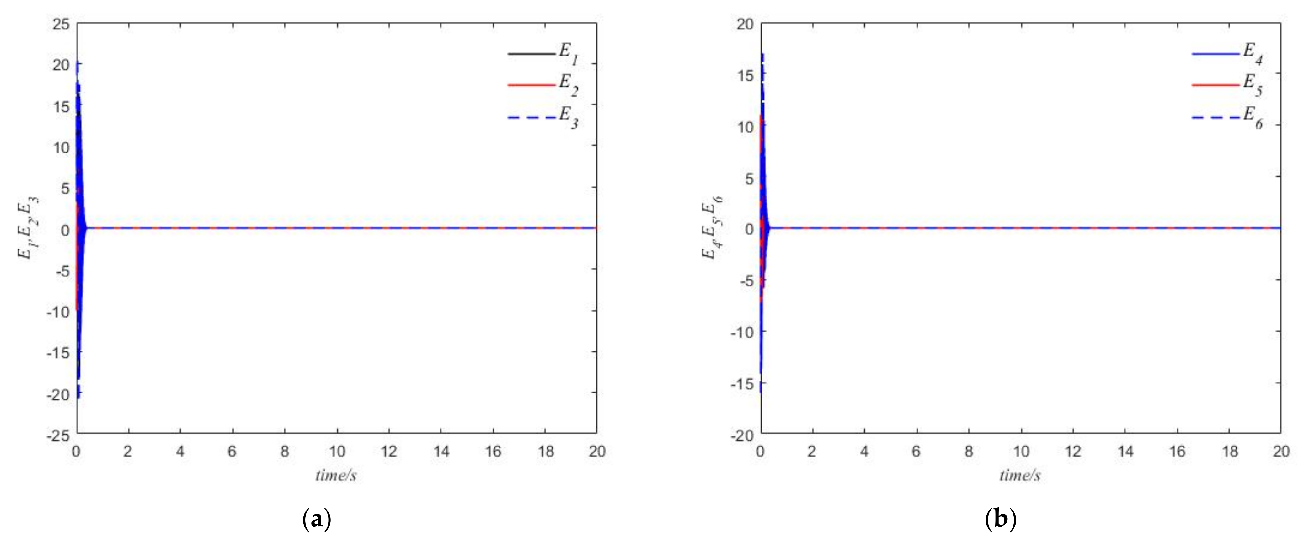
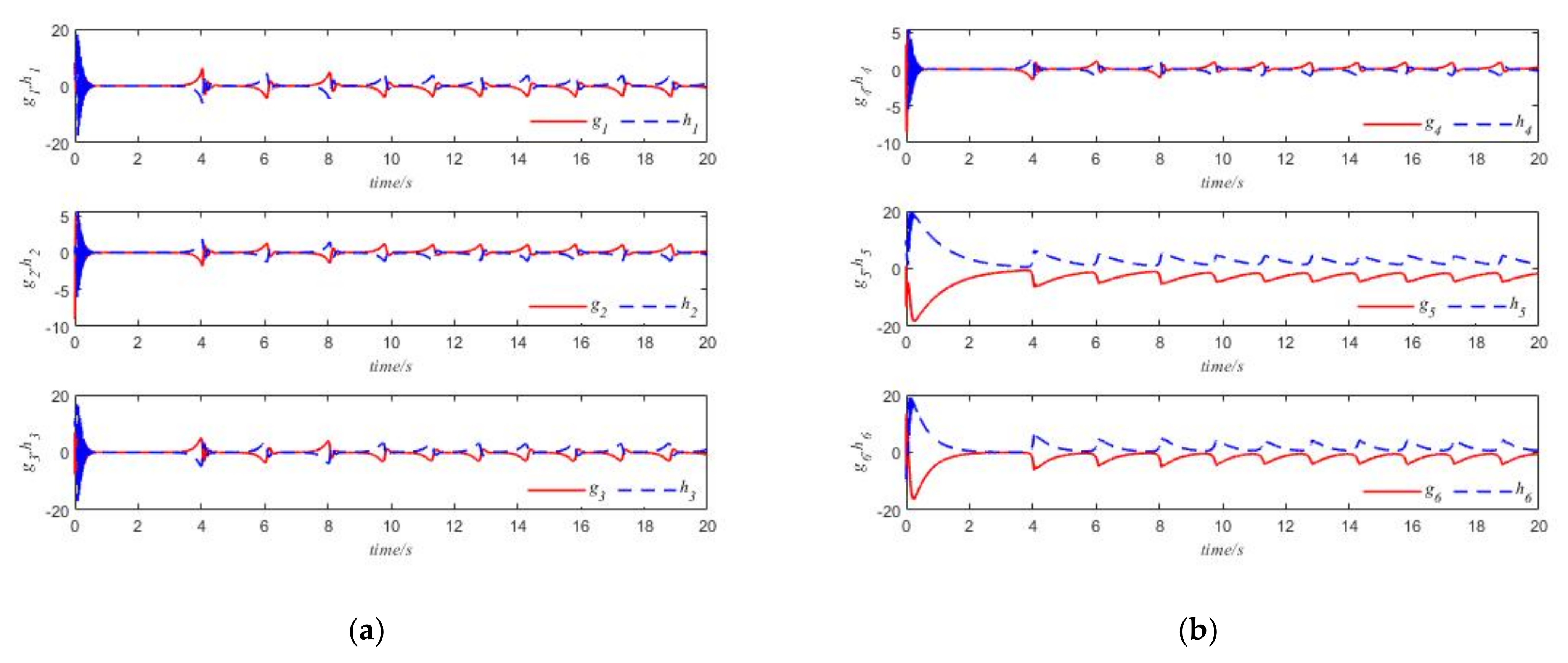
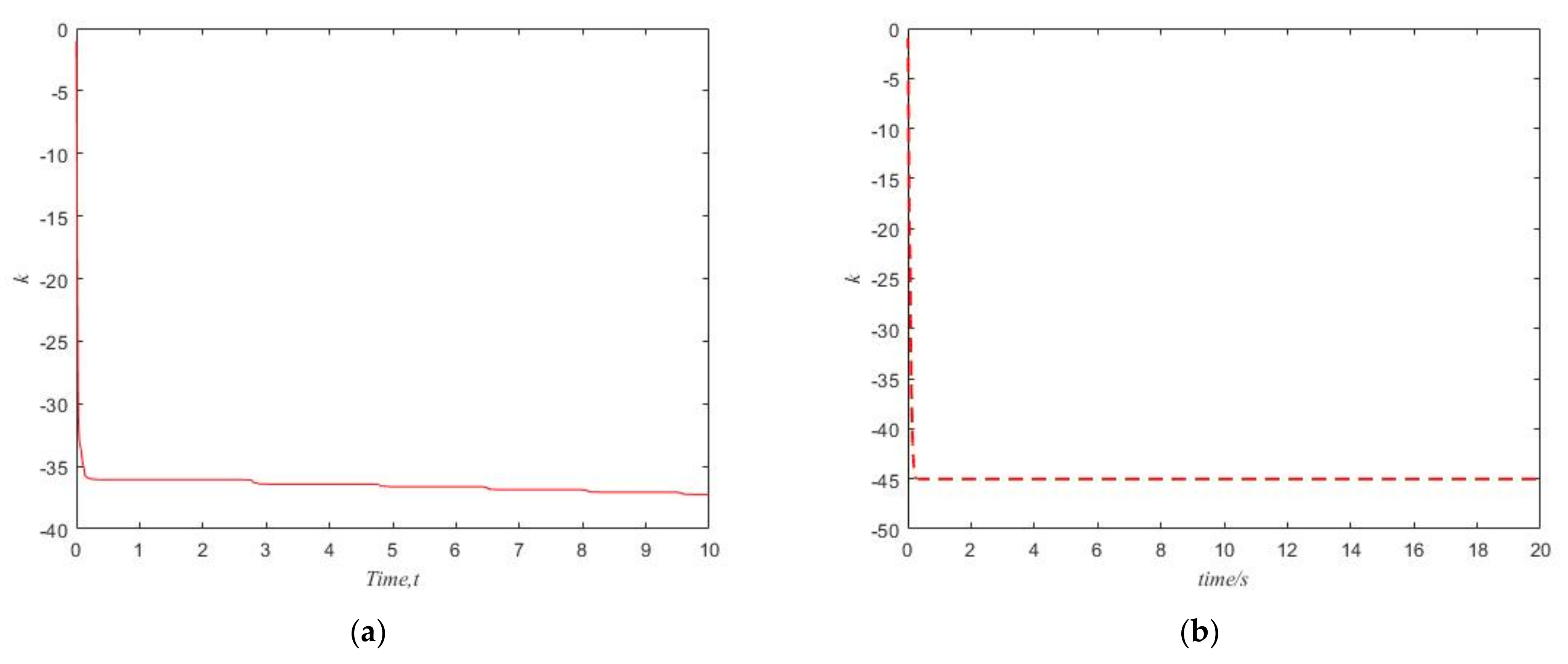
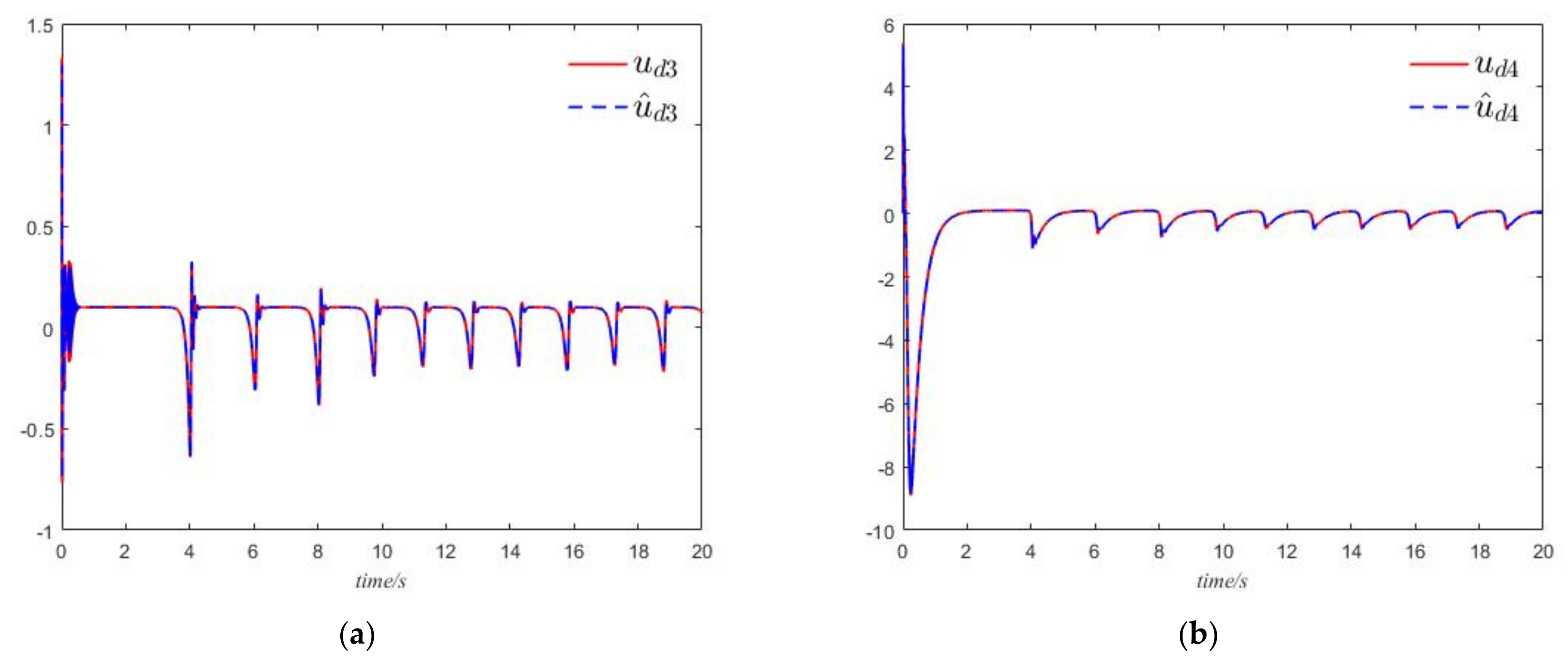
5.3. Anti-Synchronization

Numerical simulations are given, and the initial values of the master–slave systems of the given complex 4D chaotic system are chosen as follows: $g(0)=[4,-9,7,-4,1,-6],h(0)=[8,-1,9,-5,10,-10],k(0)=-1$. It can be seen from Figure 9 that the sum system is asymptotically stable. Through the observation of Figure 10, it is found that under the action of the combined controller, the master system and slave system achieve anti-synchronization. Figure 11 shows that the dynamic feedback gain of the system converges to a negative constant. By comparing the two figures, we can clearly see that after adding the UDE controller, the feedback gain approaches a fixed value with time. Figure 12 verifies that the low-pass filter in the combined controller successfully estimates the given model uncertainty and external perturbation accurately, ${\widehat{u}}_{d_1}$ tends to $u_{d_1}$ and ${\widehat{u}}_{d_2}$ tends to $u_{d_2}$. Similarly, we found that ${\widehat{u}}_{d_3}$ tends to $u_{d_3}$ and ${\widehat{u}}_{d_4}$ tends to $u_{d_3}$ from Figure 13.

6. Conclusions

In this paper, the problem of stabilization, complete synchronization, and anti-synchronization of a complex 4D hyper-chaotic system have been investigated. Firstly, the real part and imaginary part of the complex 4D chaotic system have been separated, and the system is equivalent to a six-dimensional continuous autonomous real chaotic system. Secondly, a dynamic gain feedback controller has been designed and then based on the control method of UDE, two appropriate low-pass filters are selected to complete the complete synchronization and anti-synchronization control of a given system. Finally, using MATLAB to carry out the numerical simulation, compared with the system without a UDE controller, it is not difficult to find that the stability of the system has been significantly improved after adding the combined controller, which verifies the correctness and effectiveness of the proposed results. The research method proposed in this paper can also be applied to other chaotic or hyper-chaotic systems.

References

1. Pecora, L.; Carroll, T. Synchronization in Chaotic Systems. Phys. Rev. Lett. 1990, 64, 821–824. [Google Scholar] [CrossRef] [PubMed]
2. Jalal, A.A.; Amen, A.I. Darboux integrability of the simple chaotic flow with a line equilibria differential system. Chaos Solitons Fractals 2020, 135, 109712. [Google Scholar] [CrossRef]
3. Osses, G.; Castillo, E. Numerical modeling of laminar and chaotic natural convection flows using a non-residual dynamic VMS formulation. Comput. Methods Appl. Mech. Eng. 2021, 386, 114099. [Google Scholar] [CrossRef]
4. Aidaoui, L.; Lasbet, Y. Improvement of transfer phenomena rates in open chaotic flow of nanofluid under the effect of magnetic field: Application of a combined method. Int. J. Mech. Sci. 2020, 179, 105649. [Google Scholar] [CrossRef]
5. Giona, M.; Adrover, A.; Cerbelli, S. On the use of the pulsed-convection approach for modelling advection-diffusion in chaotic flows—A prototypical example and direct numerical simulations. Physica A 2005, 348, 37–73. [Google Scholar] [CrossRef]
6. Guo, R. A simple adaptive controller for chaos and hyper-chaos synchronization. Phys. Lett. A 2008, 372, 5593–5597. [Google Scholar] [CrossRef]
7. Mahmoud, G.M.; Ahmed, M.E.; Mahmoud, E.E. Analysis of hyperchaotic complex Lorenz systems. Int. J. Mod. Phys. C 2008, 19, 1477–1494. [Google Scholar] [CrossRef]
8. Hammami, S.; Benrejeba, M.; Fekib, M.; Borne, P. Feedback control design for Rossler and Chen chaotic systems anti-synchronization. Nonlinear Dyn. 2010, 374, 2835–2840. [Google Scholar] [CrossRef]
9. Guo, R. Projective synchronization of a class of chaotic systems by dynamic feedback control method. Nonlinear Dyn. 2017, 90, 53–64. [Google Scholar] [CrossRef]
10. Jiang, W.H.; Niu, B. On the coexistence of periodic or quasi-periodic oscillations near a Hopf-pitchfork bifurcation in NFDE. Commun. Nonlinear Sci. Numer. Simul. 2013, 18, 464–477. [Google Scholar] [CrossRef]
11. Guo, R.W. Simultaneous synchrnizaiton and anti-synchronzation of two identical new 4D chaotic systems. Chin. Phys. Lett. 2011, 28, 040205. [Google Scholar] [CrossRef]
12. Dai, J.G.; Ren, B.B. UDE-based robust boundary control for an unstable parabolic PDE with unknown input disturbance. Automatica 2018, 93, 363–368. [Google Scholar] [CrossRef]
13. Ren, B.; Zhong, Q.C. Asymptotic reference tracking and disturbance rejection of UDE-based robust control. IEEE Trans. Ind. Electron. 2017, 64, 3166–3176. [Google Scholar] [CrossRef]
14. Aviram, I.; Rabinovitch, A. Bifurcation analysis of bacteria and bacteriophage coexistence in the presence of bacterial debris. Commun. Nonlinear Sci. Numer. Simul. 2012, 17, 242–254. [Google Scholar] [CrossRef]
15. Huang, C.; Cao, J. Active control strategy for synchronization and anti-synchronization of a fractional chaotic financial system. Physica A 2017, 4731, 262–275. [Google Scholar] [CrossRef]
16. Liu, D.; Zhu, S.; Sun, K. Anti-synchronization of complex-valued memristor-based delayed neural networks. Neural Netw. 2018, 105, 1–13. [Google Scholar] [CrossRef]
17. Jia, B.; Wu, Y.; He, D.; Guo, B.; Xue, L. Dynamics of transitions from anti-phase to multiple in-phase synchronizations in inhibitory coupled bursting neurons. Nonlinear Dyn. 2018, 93, 1599–1618. [Google Scholar] [CrossRef]
18. Mahmoud, E.E.; Abo-Dahab, S.M. Dynamical properties and complex anti-synchronization with applications to secure communications for a novel chaotic complex nonlinear model. Chaos Solitons Fractals 2018, 106, 273–284. [Google Scholar] [CrossRef]
19. Mahmoud, E.E. Dynamical behaviors, Control and synchronization of a new chaotic model with complex variables and cubic nonlinear terms. Results Phys. 2017, 10, 1346–1356. [Google Scholar] [CrossRef]
20. Yang, D.X.; Zhou, J.L. Connections among several chaos feedback control approaches and chaotic vibration control of mechanical systems. Commun. Nonlinear Sci. Numer. Simul. 2014, 19, 3954–3968. [Google Scholar] [CrossRef]
21. Huang, Y.; Hou, J.; Yang, E. General decay lag anti-synchronization of multi-weighted delayed coupled neural networks with reaction-diffusion terms. Inf. Sci. 2020, 511, 36–57. [Google Scholar] [CrossRef]
22. Pecora, L.M.; Carroll, T.L. Synchronization of chaotic systems. Chaos 2015, 25, 597–611. [Google Scholar] [CrossRef] [PubMed]
23. Ren, L.; Guo, R.W. A necessary and sufficient condition of anti-synchronization for chaotic systems and its applications. Math. Probl. Eng. 2015, 2015, 1–7. [Google Scholar]
24. Jiang, H.B.; Liu, Y.; Zhang, L.P.; Yu, J.J. Anti-phase synchronization and symmetry-breaking bifurcation of impulsively coupled oscillators. Commun. Nonlinear Sci. Numer. Simul. 2016, 39, 199–208. [Google Scholar] [CrossRef] [Green Version]
25. Mobayen, S. Chaos synchronization of uncertain chaotic systems using composite nonlinear feedback based integral sliding mode control. ISA Trans. 2018, 77, 100–111. [Google Scholar] [CrossRef] [PubMed]
26. Mobayen, S. A novel global sliding mode control based on exponential reaching law for a class of underactuated systems with external disturbances. J. Comput. Nonlinear Dyn. 2015, 11, 021011. [Google Scholar] [CrossRef]
27. Yi, X.; Guo, R.; Qi, Y. Stabilization of Chaotic Systems with Both Uncertainty and Disturbance by the UDE-Based Control Method. IEEE Access 2020, 8, 62471–62477. [Google Scholar] [CrossRef]
28. Li, L.; Li, B.; Guo, R. Consensus Control for Networked Manipulators with Switched Parameters and Topologies. IEEE Access 2021, 9, 9209–9217. [Google Scholar] [CrossRef]
29. Peng, R.; Jiang, C.; Guo, R. Stabilization of a class of fractional order systems with both uncertainty and disturbance. IEEE Access 2021, 9, 42697–42706. [Google Scholar] [CrossRef]
Figure 1. The states of the system are asymptotically stable. (a) g1, g2, g3 are asymptotically stable; (b) g4, g5, g6 are asymptotically stable.
Mathematics 10 01313 g001
Figure 2. The feedback gain asymptotically converges to a negative constant. (a) without UDE control; (b) UDE control.
Mathematics 10 01313 g002
Figure 3. Uncertainty and disturbance term u d 1 and its estimation u ^ d 1 .
Mathematics 10 01313 g003
Figure 4. Error systems when the controller has been activated, showing that e1, e2, e3, e4, e5, e6 are stabilized, implying that the existence of complete synchronization in the complex nonlinear system is realized. (a) e1, e2, e3 are asymptotically stable; (b) e4, e5, e6 are asymptotically stable.
Mathematics 10 01313 g004
Figure 5. Dynamics of the state variables when controller has been activated, the master system and slave system achieve the complete synchronization. (a) g1, g2, g3 synchronize the states h1, h2, h3; (b) g4, g5, g6 synchronize the states h4, h5, h6.
Mathematics 10 01313 g005
Figure 6. The feedback gain asymptotically converges to a negative constant. (a) without UDE control; (b) UDE control.
Mathematics 10 01313 g006
Figure 7. Uncertainty and disturbance u d 1 , u d 2 and their estimated value, gradually tend to be the same. (a) u ^ d 1 tends to u d 1 ; (b) u ^ d 2 tends to u d 2 .
Mathematics 10 01313 g007
Figure 8. u d 3 and its estimated value u ^ d 3 .
Mathematics 10 01313 g008
Figure 9. Error systems when the controller has been activated, showing that E1, E2, E3, E4, E5, E6 are stabilized, implying that the existence of anti-synchronization in the complex nonlinear system is realized. (a) E1, E2, E3 are asymptotically stable; (b) E4, E5, E6 are asymptotically stable.
Mathematics 10 01313 g009
Figure 10. Dynamics of the state variables when controller has been activated, the master system and slave system achieve the anti-synchronization. (a) g1, g2, g3 anti-synchronize the states h1, h2, h3; (b) g4, g5, g6 anti-synchronize the states h4, h5, h6.
Mathematics 10 01313 g010
Figure 11. The feedback gain asymptotically converges to a negative constant. (a) without UDE control; (b) UDE control.
Mathematics 10 01313 g011
Figure 12. Uncertainty and disturbance u d 1 , u d 2 and their estimated value, gradually tend to be the same. (a) u ^ d 1 tends to u d 1 ; (b) u ^ d 2 tends to u d 2 .
Mathematics 10 01313 g012
Figure 13. Uncertainty and disturbance u d 3 , u d 4 and their estimated value, gradually tend to be the same. (a) u ^ d 3 tends to u d 3 ; (b) u ^ d 4 tends to u d 4 .
Mathematics 10 01313 g013
Publisher’s Note: MDPI stays neutral with regard to jurisdictional claims in published maps and institutional affiliations.