Inferring from References with Differences for Semi-Supervised Node Classification on Graphs

Abstract

Following the application of Deep Learning to graphic data, Graph Neural Networks (GNNs) have become the dominant method for Node Classification on graphs in recent years. To assign nodes with preset labels, most GNNs inherit the end-to-end way of Deep Learning in which node features are input to models while labels of pre-classified nodes are used for supervised learning. However, while these methods can make full use of node features and their associations, they treat labels separately and ignore the structural information of those labels. To utilize information on label structures, this paper proposes a method called 3ference that infers from references with differences. Specifically, 3ference predicts what label a node has according to the features of that node in concatenation with both features and labels of its relevant nodes. With the additional information on labels of relevant nodes, 3ference captures the transition pattern of labels between nodes, as subsequent analysis and visualization revealed. Experiments on a synthetic graph and seven real-world graphs proved that this knowledge about label associations helps 3ference to predict accurately with fewer parameters, fewer pre-classified nodes, and varying label patterns compared with GNNs.

1. Introduction

In classification tasks where we assign labels to data points according to their features, Neural Networks using Deep Learning [1] are optimized to fit the mapping from features to labels. As an application of Deep Learning to relational data where data points are illustrated as nodes and their relations are denoted as the edges between nodes, Graph Neural Networks (GNNs) [2] utilize the structural information coming from relations to predict a data point’s label according to its and its related data points’ features, such as the Graph Convolutional Network (GCN) [3], Graph Attention Network (GAT) [4], and Approximate Personalized Propagation of Neural Predictions (APPNP) [5]. Such a utilization is limited. While GNNs make full use of node features and their associations, they treat labels separately and ignore the structural information of labels.

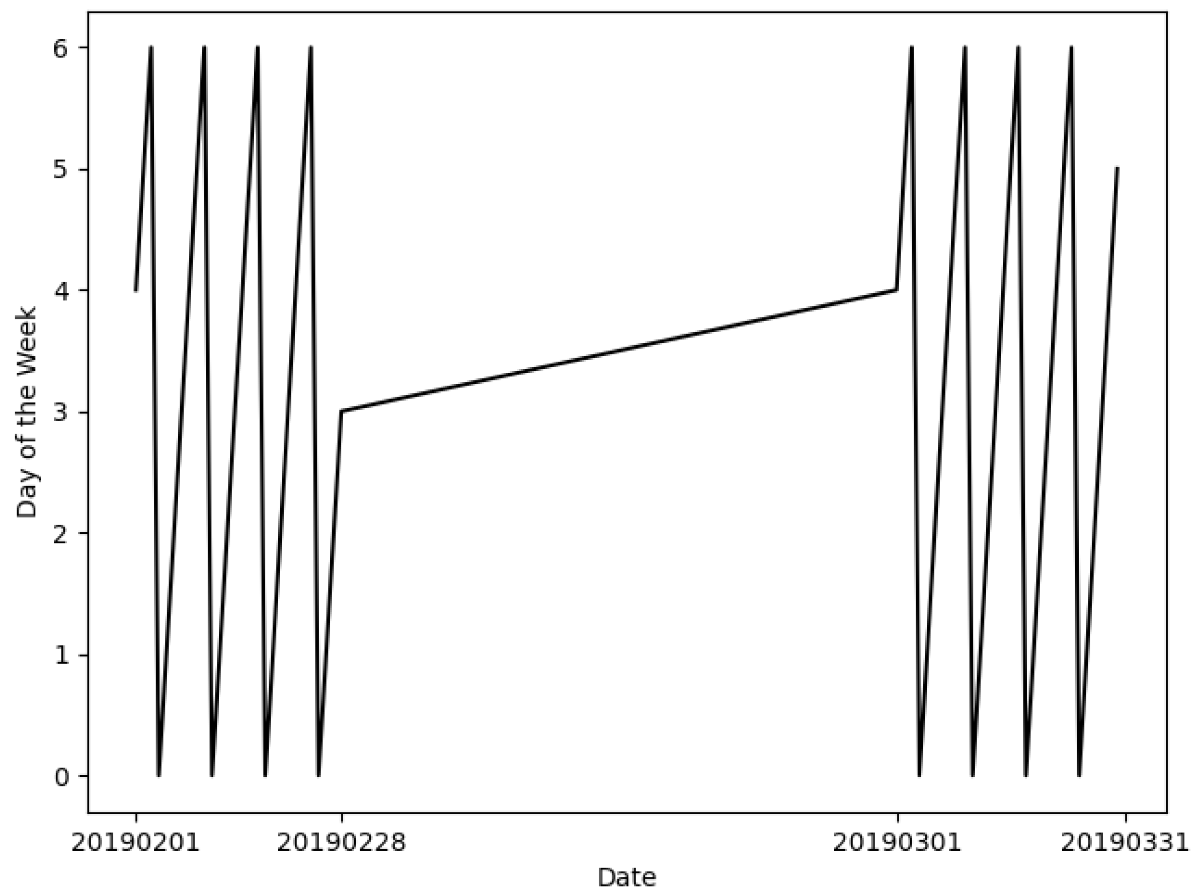
The omitted information of label structures may be crucial to the tasks. For example, most people have no idea when answering ‘What day is 2 September 1984’, while they immediately know it is Sunday if informed that 8 September 1984 is Saturday. The human logic behind this Weekday Prediction task is to infer the answer from a related known fact as the reference with their difference, as:

• The reference: ‘8 September 1984 is Saturday’;
• The difference: ‘there are 6 days from 2 September 1984 to 8 September 1984’;
• The inference: ‘2 September 1984 is Sunday’.

On the contrary, Neural Networks resolve this task by approximating the mapping from dates to days of the week, which can be formulated with Zeller’s congruence [6]:

$$h=(q+\lfloor \frac{13(m+1)}{5}\rfloor +K+\lfloor \frac{K}{4}\rfloor +\lfloor \frac{J}{4}\rfloor -2J-2)\mathrm{mod}7$$

where h is the day of the week (0 for Monday, 1 for Tuesday, etc.), q is the day of the month (1 for 1st, 2 for 2nd, etc.), m is the month (1 for January, 2 for February, etc.), K is the year of the century, J is the zero-based century, and $\lfloor ·\rfloor$ is the integer part of a number. Due to the $\lfloor ·\rfloor$ function and the mod operation, this mapping is a piecewise continuous function with many nonlinearities (Figure 1). Neural Networks and Graph Neural Networks have to own excessive numbers of activators and parameters to fit all continuous sections of this mapping [7].

Therefore, in addition to associations between features, some recent works have also considered associations between labels. Most of them inherit a heuristic method called the Label Propagation Algorithm (LPA) [8], which propagates labels from labeled nodes to unlabeled ones, assuming that related data points share similar labels. For example, GCN-LPA [9] transfers the optimized relation weights from LPA into a GCN model to strengthen the connection between same-labeled data points and tell ambiguous data points apart. Correct and Smooth (C&S) [10] boosts its base predictor by propagating the differences between the ground-truth labels and the predicted labels. The ResLPA [11] fits the differences (or residuals) between connected data points’ labels and then labels unlabeled data points according to their labeled neighbors.

However, LPA’s assumption that adjacent nodes label alike does not always hold. Take the Weekday Prediction as an example. Days of the week vary between adjacent dates, so LPA and LPA-based methods such as GCN-LPA, C&S, and The ResLPA cannot obtain the correct day of the week by propagating days of the week from nearby dates. Subsequent works such as UniMP [12] and the Label Input trick [13] avoid this assumption of LPA by inputting both labels and features into GNNs. Benefiting from the ability of Neural Networks inside GNNs, these methods capture the hidden pattern of labels and extend GNNs to suit graphs with varying label patterns. Meanwhile, another issue is raised. Input labels may cause information leakage and prevent GNNs from learning. UniMP and the Label Input trick resolve the issue by dividing known labels into inputting labels and supervising labels. This trade-off shrinks the scale of the training set and leaves training data without full utilization.

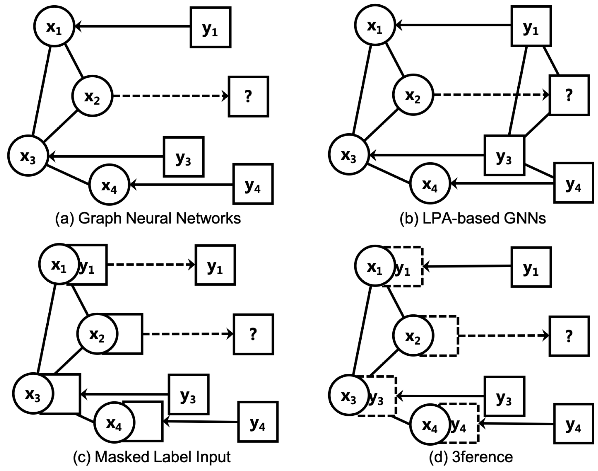
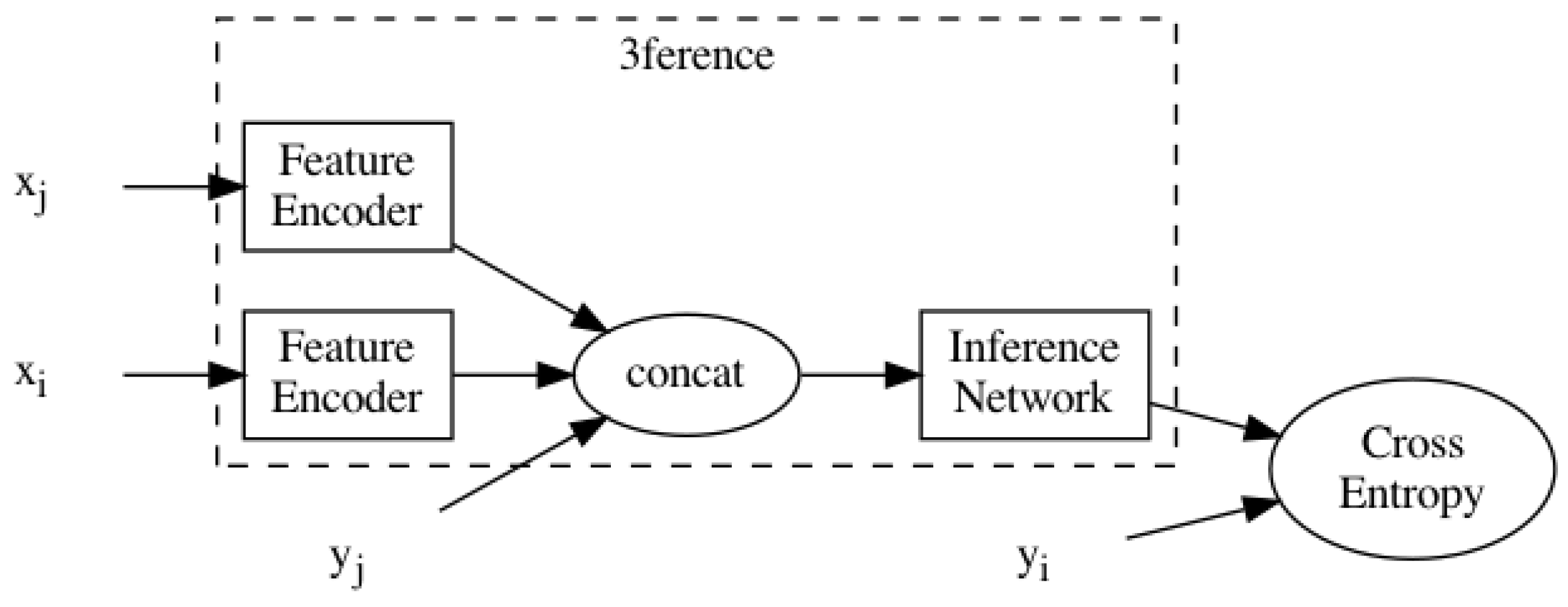
Inspired by the way people figure out weekdays, we propose a method named 3ference as inferring from references with differences to incorporate information from graph structures, node features, and node labels. In contrast to the aforementioned methods shown in

Table 1. Comparison among graph learning models on how many labels are input and whether a model is suitable for various label patterns. C&S assumes that adjacent nodes have similar residuals between the ground-truth labels and the outputs of the base predictor.

Methods	No	Input Label Partial	All	Label Pattern Any
LPA			✓	✕
GCN	✓			✓
GAT	✓			✓
APPNP	✓			✓
GCN-LPA			✓	✕
C&S			✓	✕
ResLPA			✓	✕
UniMP		✓		✓
Label Input		✓		✓
3ference			✓	✓

, 3ference fully leverages labels that may be in complex patterns. To infer the label of a target data point (or node), 3ference employs its labeled related data points (or labeled adjacent nodes) as references and then combines the features of the target, the features of the references, and the labels of the references to compute the label distribution of the target. This difference between conventional end-to-end methods and 3ference is shown in Figure 2. By utilizing labels from references, 3ference can capture the pattern of labels in data points, reducing the burden of predicting labels entirely with features [14].

In this article, we first introduce the task of Node Classification on graphs of data points and categorize mainstream approaches to solve this task into LPA, GNNs, their integrations, and label tricks in Section 3. We then formulate the 3ference method and its efficient variant in Section 4. After that, we experiment with 3ference in Weekday Prediction and Node Classification in Section 5, proving that 3ference can overcome the complexity of tasks with the help of references and remain effective when the parameters are few or when the label pattern changes. After that, we visualize the label transition matrices and a trained 3ference’s weight matrices, suggesting that 3ference successfully recovers the associations between labels and predicts based on them with approximated differences. Finally, we conclude with some inspirations and future directions in Section 6.

2. Preliminaries

A graph G is defined as the combination of a node set $V=\{v_1,v_2,\cdots v_n\}$ and an edge set $E=\left\{(i,j)\right|v_i\mathrm{and}{v}_j\mathrm{are}\mathrm{connected}\}$. In numerous real-world fields, this kind of data is capable of describing entities and their relations. For example, citation networks can be represented as graphs where the node set contains all the documents and the edge set contains all connections between document pairs if one cites another. Likewise, social networks of people with their friendship, biological networks of proteins with their associations, and recommender systems of goods with their co-purchase events can all be represented in graphs. In general, a node $v_i$ in a graph is attached with a d-dimensional vector $x_i$ of features (bag-of-words encodes of documents, etc.) that V is represented by a feature matrix $X\in {\mathbb{R}}^{n\times d}$. The edge set E is represented by an adjacency matrix $A\in {\{0,1\}}^{n\times n}$. The entry $a_{ij}\in \{0,1\}$ in the i-th row and j-th column in A represents a connection from node $v_i$ to $v_j$.

Because of this flexibility of representation, graphic data are widely used. Mining information from graphic data has drawn much attention in recent years. In this work, we concentrate on the Node Classification task of this area. Given a graph $G=(V,E)=(A,X)$, c labels, and a training set $L\subset V$ with m nodes that are already assigned with labels $Y^L\in {\{0,1\}}^{m\times c}$, $Y^L$ is a label matrix where each row of it is a one-hot vector indicating to which label the corresponding node is assigned. The goal of Node Classification is to classify the rest of the unlabeled nodes by assigning labels to them. This task is versatile. For example, in citation networks, we can classify documents by fields of study. In social networks, we may classify people by their interests. In biological networks, we can classify proteins by species. In these scenarios, labels can be study fields, communities, and species.

3. Related Works

Many approaches have been proposed to solve Node Classification in the graph domain. The main two parallel families of approaches are the Label Propagation Algorithm (LPA) [8] and Graph Neural Networks (GNNs) [2].

LPA assumes that adjacent nodes in the graph share similar labels. It propagates label information from nodes in the training set where nodes are labeled to their adjacent neighbors iteratively. After several propagating steps, unlabeled nodes can gather enough label information from their neighborhood. Their labels can then be determined by aggregated information. We form the label matrix $Y\in {\{0,1\}}^{n\times c}$. If $v_i\in L$, then the i-th row $Y_i$ of Y is a one-hot vector indicating $v_i$’s label. Otherwise, the c elements of $Y_i$ are all 0. LPA can then be described by the following formulas:

$$\begin{array}{cc}\hfill Y& =(1-\alpha )·Y+\alpha ·D^{-1}AY\hfill \\ \hfill Y_i& =Y_i^L,\forall v_i\in L\hfill \end{array}$$

where $\alpha \in (0,1)$ is a hyperparameter and D is a diagonal matrix with diagonal entries $\{d_i={\displaystyle \sum _{j=1}^n}{a}_{ij}|i=1,2,\cdots ,n\}$. While LPA is efficient and easy to implement, it relies on the assumption that adjacent nodes share similar labels. Moreover, it cannot take full advantage of feature information X.

Graph Neural Networks (GNNs) overcome these drawbacks and bring deep learning techniques into graphs. They learn the representations of nodes from transformed features in a message-passing scheme and update model parameters by propagating back the loss of predicted labels on the training data. GNNs have many varieties, among which a one-layered Graph Convolutional Network (GCN) [3] can be formulated as:

$$Y=\sigma \left(D^{-1}AXW\right)$$

where $\sigma$ is the sigmoid function. Subsequent works include the Graph Attention Network (GAT) [4], which computes edge weights to adaptively filter propagating representations, the Approximate Personalized Propagation of Neural Predictions (APPNP) [5], which decouples the transformation procedure and the propagation procedure [15] of GCN, and so on. Because of the good performance and many other advantages, GNNs are now dominant methods for solving Node Classification. However, most GNNs concentrate mainly on the association of node features, while ignoring the associations of node labels.

To exploit label information more, recent studies such as GCN-LPA [9], Correct and Smooth (C&S) [10], and the ResLPA [11] integrates both the LPA and GNNs, revealing the ties between them in theory and matching or exceeding many state-of-the-art GNNs on a wide variety of benchmarks in practice. The GCN-LPA considersthe LPA and GCN in terms of influence [16] and proves the quantitative relationship between them. As an application of its theory, it regularizes the GCN with the learned edge weights that optimize the LPA. It assists the GCN in separating nodes with different labels, resulting in benefits to Node Classification. C&S first employs a simple base predictor such as Multi-Layer Perceptron (MLP) [17] or the GCN to predict labels. Assuming the predicting errors are close on adjacent nodes, it then corrects these predictions by minus prediction errors propagated from the training set (labeled nodes) to the testing set (unlabeled nodes). After that, it casts another LPA as its smooth procedure to propagate the corrected predictions. This combination of a base predictor and two LPAs results significant performance on various Open Graph Benchmark (OGB) datasets [18]. The ResLPA propagates label distributions as the LPA does. In addition, it adds label residuals approximated from node features with a simple network. However, because the LPA is nonparametric, these simple combinations of the LPA and GNNs may lead to suboptimal results or heavy tuning on $\alpha$. Moreover, these methods are restricted by the assumption of the LPA. When adjacent nodes tend to have different labels, such as Weekday Prediction, these methods may be rendered ineffective.

To rectify this issue, researchers apply the Label Input trick [13] to incorporate both features and labels without assuming the pattern of labels. The Label Input trick divides the training set into multiple parts. It concatenates node features with some parts of the training set and feeds them into a foundational GNN to recover the rest of the divided training set. Subsequent theoretical analysis [19] proved that the Label Input trick serves as a regularization of the training objective conditioned on graph size and connectivity. Label Reuse [13] is another trick for labels that researchers commonly adopt based on the Label Input trick. It iterates the foundational GNN model several times. In every iteration, the predicted results are reused as inputs like the Label Input trick to produce new results in the next iteration. The Label Reuse trick relieves the inherent asymmetry of the Label Input trick between input one-hot labels for labeled nodes and all-zero placeholders for unlabeled nodes. The Label Input trick and the Label Reuse trick can be applied to any foundational GNN models to exploit label information without modifications to the GNNs. For example, many top-ranking submissions on the OGB leaderboard use these two tricks, among which UniMP [12] applies the Label Input trick on a multi-layered Graph Transformer [20]. For supervising purposes, a considerable part of the labels from the training set is masked and cannot be input into the foundational GNN. The structural information of these labels is thus missing.

4. Proposed Approach

In this section, we propose the method of 3ference and the way to train it in mini-batches.

4.1. 3ference

We borrow the ResLPA’s theory that a node’s label can be inferred from the labels of its neighbors and their features. Given a central node $v_i$ and its neighborhood $N_i=\left\{v_j\right|a_{ij}=1\}$, we predict the label distribution $y_i$ of $v_i$ by aggregating the information including labels from its adjacent nodes:

$$\begin{array}{cc}\hfill z_i& =\frac{1}{|N_i|}·\sum _{v_j\in N_i}{f}_{\theta }(x_i,x_j,y_j)\hfill \\ \hfill {\widehat{y}}_i& =\mathrm{Softmax}\left(z_i\right)\hfill \end{array}$$

where $f_{\theta }$ is the 3ference network, $|N_i|$ is the cardinality of the set $N_i$, and $\mathrm{Softmax}(·)$ is a function that rescales the input c-dimensional array h so that every rescaled element lies in the range $[0,1]$, while all of them sum to 1:

$$\mathrm{Softmax}\left(h\right)=\frac{(e^{h_1},e^{h_2},\cdots ,e^{h_c})}{{\displaystyle \sum _{i=1}^c}{e}^{h_i}}$$

The architecture of the 3ference network is illustrated in Figure 3. For every node $v_j$ that is adjacent to node $v_i$, node features $x_j$ and $x_i$ are encoded by the Feature Encoder and sent to the Inference Network in concatenation with the adjacent node $v_j$’s label distribution $y_j$. We implemented both Feature Encoders and the Inference Network as Multi-Layer Perceptrons (MLPs). If $v_j$ is not in the training set and the label of $v_j$ is not given, ${\widehat{y}}_j$ from the last iteration or the initial vector 0 is reused, as the Label Reuse trick does. We average the results for all $v_j$ to produce the aggregated logits $z_i$ and normalize it to obtain the estimated label distribution ${\widehat{y}}_i$ of node $v_i$ with the Softmax function. The loss of predicted label distributions is then computed via Cross-Entropy and optimized with Gradient Descendent:

$$l=\mathrm{CrossEntropy}(y_i^L,{\widehat{y}}_i)=-\sum _{j=1}^c{y}_{ij}^{L}log{\widehat{y}}_{ij}$$

We describe the method of 3ference with Algorithm 1. From Line 1 to Line 3 in the algorithm, we initialize the label distributions $\widehat{Y}$ of all nodes. If a node $v_i$ is in the training set, we populate the i-th row ${\widehat{Y}}_i$ with the one-hot label indicator from $Y^L$. Otherwise, the elements of that row are all 0. From Line 5 to Line 10, we optimize the 3ference network $f_{\theta }$ to infer from adjacent references with their labels as inputs and the central node’s label as supervision. This procedure is similar to the Label Input trick. However, different from that, 3ference makes full use of labels in the training set since it only masks the target node’s label for supervising purposes. From Line 11 to Line 14, we predict the label distributions outside of the training set. Similar to the Label Reuse trick, the predictions are reused as references in the following training cycle.

Algorithm 1 The 3ference algorithm.
Input: adjacency matrix A, node features X, and training labels $Y^L$. Parameter: 3ference network $f_{\theta }$.
Output: predicted label distributions $\widehat{Y}$.
1:	for  $\forall v_i\in L$  do
2:	${\widehat{Y}}_i=\left\{\begin{array}{c}{Y}_i^L,v_i\in L\hfill \\ 0,\mathrm{otherwise}\hfill \end{array}\right.$
3:	end for
4:	for $t=1,\cdots ,T$  do
5:	for $\forall v_i\in L$ do
6:	$z_i=\frac{1}{|N_i|}·{\displaystyle \sum _{v_j\in N_i}}{f}_{\theta }(x_i,x_j,{\widehat{Y}}_j)$
7:	${\widehat{Y}}_i=\mathrm{Softmax}\left(z_i\right)$
8:	l = CrossEntropy($Y_i^L,{\widehat{Y}}_i$)
9:	$\theta =\theta -\beta ·\frac{\partial l}{\partial \theta }$.
10:	end for
	// propagate predicted label distributions
11:	for $\forall v_i\in V-L$ do
12:	$z_i=\frac{1}{|N_i|}·{\displaystyle \sum _{v_j\in N_i}}{f}_{\theta }(x_i,x_j,{\widehat{Y}}_j)$
13:	${\widehat{Y}}_i=\mathrm{Softmax}\left(z_i\right)$
14:	end for
15:	end for
16:	return $\widehat{Y}$.

4.2. Mini-Batch 3ference

The vanilla 3ference cannot utilize the power of the GPU directly because different nodes in a graph may have a varying amount of adjacent neighbors. To resolve this issue, we constructed a Truncated Adjacency Matrix $\tilde{A}$ and a corresponding Mask Matrix M to assist the batched training of 3ference. In $\tilde{A}$, the i-th row ${\tilde{A}}_i$ indicates a set of nodes ${\tilde{N}}_i$ that contains at most k adjacent nodes of $v_i$. If the size of $N_i$ is less than k, ${\tilde{N}}_i$ is populated with random nodes until it has k elements. The Mask Matrix M has the same shape as $\tilde{A}$. Each element $M_{ij}$ indicates whether ${\tilde{A}}_{ij}$ is a padding element.

Figure 4 illustrates an instance of constructing the truncated adjacency matrix and the Mask Matrix for a given graph. By default, we set k to be approximately equal to the ratio of the number of edges and the number of nodes.

The predicted logit $z_i$ is then formulated as:

$$z_i=\frac{1}{({\tilde{A}}_i,1-M_i)}·\sum _{v_j\in {\tilde{N}}_i}(1-M_{ij})·f_{\theta }(x_i,x_j,y_j)$$

where $({\tilde{A}}_i,1-M_i)$ is the inner product of the i-th rows of $\tilde{A}$ and $1-M$.

5. Experiments

In this section, We compare 3ference against seven baselines on one synthetic dataset and seven real-world datasets (code for experiments: https://github.com/cf020031308/3ference, accessed on 9 April 2022). To carefully compare the various methods, we conducted the Node Classification experiment with different numbers of parameters and datasets split.

5.1. Datasets

We conducted Node Classification experiments on a synthetic network, three citation networks, two co-authorship networks, and two co-purchase networks to fully evaluate our methods.

Weekday. We generated 14,610 dates ranging from January 1st in 1980 to November 31th in 2019 as 8-dimensional vectors. Each date is labeled as a scalar from 0 to 6 to represent its corresponding day of the week. For example, the date September 2nd in 1984 has a feature vector (1, 9, 8, 4, 0, 9, 0, 2) an assigned label 0 (Sunday). Each date is represented as a node connecting to the other four nearest nodes under the Euclidean distance of features to convert Weekday Prediction to Node Classification.

Citation networks. We experimented with our methods on three citation networks named Cora, Citeseer, and Pubmed [21]. In these graphs, nodes represent academic papers. Words of papers are extracted and encoded into vectors of features. Each node is assigned a label that indicates the paper’s research field. If one paper cites another, their nodes are connected.

Co-purchase networks. Nodes in the two co-purchase networks Amazon Photo and Amazon Computer [22] represent goods for sale on e-commerce websites. Node features encode words of goods’ descriptions. Node labels are assigned according to the categories of the goods. Connections indicate that the two connected goods are frequently bought together.

Co-authorship networks are graphs of researchers and their co-authorship. The encodings of words in a researcher’s papers construct the node’s features. The researcher’s study field constructs the node’s label. If two researchers have co-authored any paper, their nodes will be connected. The two co-authorship networks we used in this work are Coauthor CS and Coauthor Physics [23,24].

We summarize some features of these datasets in

Table 2. A summary of the eight graphs. These graphs are different in many respects, such as the dataset scale, the edge density, the graph connectivity, and the label relevance.

	#Nodes	#Features	#Classes	#Edges	Average Degrees	Maximal Connected Subgraphs	Intra-Class Edge Rate
Weekday	14,610	8	7	58,440	4.00	2	1.44%
Cora	2708	1433	7	5278	3.90	78	81.00%
Citeseer	3327	3703	6	4552	2.77	438	73.91%
Pubmed	19,717	500	3	44,324	4.50	1	80.24%
Amazon Photo	7650	745	8	119,081	31.13	136	82.72%
Amazon Computer	13,752	767	10	245,861	35.76	314	77.72%
Coauthor CS	18,333	6805	15	81,894	8.93	1	80.81%
Coauthor Physics	34,493	8415	5	247,962	14.38	1	93.14%

. As we can see, these datasets are different in many respects. Cora and Citeseer are small-scale graphs. Citeseer and the two co-purchase networks are partitioned into many parts. This poor connectivity may make information propagating or message passing difficult. Co-authorship networks are rich in features where the utilization of features may be more important than that of structural information.

Specifically, we compute the Intra-Class Edge Rate [9] as the percentage of connections in which two nodes share the same label. It measures how well a dataset satisfies the LPA’s assumption that adjacent nodes share similar labels. As we can see, the intra-class edge rate of Weekday is far less than that of other datasets because adjacent dates have different days of the week. Therefore, LPA-based approaches may not work well in Weekday Prediction.

5.2. Baselines

We compared 3ference against the MLP [17], GCN [3], GCN + Label Input, GCN + Label Reuse [13], LPA [8], C&S [10], and Fast ResLPA [11]. For simplicity and impartial tuning, we implemented all these methods without using any regularization techniques such as Dropout [25] or Batch Normalization [26] while maintaining their amounts of parameters roughly the same. All activators between layers are LeakyReLU [27] functions.

Both implementations of the MLP and GCN have two layers. The first layer encodes the input features into h-dimensional hidden representations. The second layer maps them to c-dimensional logits of labels. In GCN + Label Input, we divide the training set into two halves, one as inputs and one for supervising. In GCN + Label Reuse, we reuse the predicted label distributions for one iteration. C&S reuses the MLP as its base predictor. The Fast ResLPA implementation is the same as the original paper [11]. In the 3ference, the feature encoder is a one-layered linear transformation that encodes the input features into h-dimensional hidden representations. The inference network is also a one-layered linear transformation to obtain c-dimensional label logits. In the LPA-based models, every propagation loop contains 50 iterations. We searched the set $\{0.1,0.2,\cdots ,0.9\}$ for the best $\alpha$ on Cora when $h=64$ and obtained 0.4 for the LPA, 0.9 for the Fast ResLPA, and 0.1 for the C&S.

5.3. Settings

The GCN and the Fast ResLPA were trained in full batches. The MLP, C&S, and 3ference were trained in mini-batches with the batch size = 1024. Except for the LPA, we optimized the cross-entropy of predictions and the ground-truth for 200 epochs using Adam [28] with the learning rate set to 0.01.

Each dataset was split into three sets. A training set contains s percent of all nodes. Rest nodes were equally divided into a validation set and a testing set. After every epoch of training or every propagation step, we evaluated the classifiers on the validation set and the testing set, producing a pair of accuracy scores. After running, the accuracy score of the testing set paired with the highest accuracy score of the validation set was noted as the score of the evaluated method. We ran each method on every dataset ten times to obtain the average score as the final result.

5.4. Results

5.4.1. Prediction Accuracy

We report the accuracy scores of the seven baselines and 3ference for Node Classification on the eight datasets in

Table 3. Accuracy scores (%) for Node Classification when $s=60$ percent of nodes are used for training and the size h of hidden representations is 64. We bold the top score on every dataset. The score of Fast ResLPA on Coauthor Physics is ‘-’ because it runs out of our GPU’s 11GB of memory.

	Weekday	Cora	Citeseer	Pubmed	Amazon Photo	Amazon Computer	Coauthor CS	Coauthor Physics
MLP	13.54	74.90	72.63	87.55	91.96	84.63	95.63	96.55
GCN	14.02	88.00	76.05	87.31	93.91	90.49	93.32	96.37
GCN + Label Input	33.20	87.49	74.48	86.41	93.68	90.57	92.69	96.03
GCN + Label Reuse	14.58	87.54	74.42	84.69	93.79	90.44	92.69	95.99
LPA	1.45	84.75	67.20	82.27	90.79	87.92	91.18	95.45
C&S	10.16	87.50	74.77	84.67	89.10	82.95	91.72	95.27
Fast ResLPA	10.74	88.10	75.73	86.73	87.84	80.67	96.03	-
3ference	51.61	87.78	76.33	88.90	95.05	90.74	95.99	97.22

. As this table shows, 3ference can consistently match or exceed other methods on most real-world datasets and produce a dominant performance in Weekday Prediction.

Since a random guess in Weekday Prediction can achieve about $1/7\approx 14.29\%$ accuracy, baselines except for GCN + Label Input all fail to predict weekdays, especially those LPA-based methods such as the LPA, C&S, and Fast ResLPA. Weekday Prediction is difficult, not only because the mapping from dates to days of the week is complex, but also because the pattern of labels differs from what the LPA and most GNNs assume. In conclusion, graph learning methods have to capture the pattern of labels instead of assuming it to gain the flexibility of applying to more situations.

Another drawback of the LPA-based methods is that we have to tune the hyperparameter $\alpha$ on every dataset to achieve the best accuracy score. The existence of hyperparameters increases the workload of deploying models on different datasets. Furthermore, this additional work of tuning makes it unfair when comparing against other adaptive models with less or no hyperparameters such as the GCN. As is seen in the table, C&S and the Fast ResLPA can obtain high scores on Cora, where their $\alpha$s are fine-tuned. However, these $\alpha$s may be suboptimal on other datasets, making them less competitive with 3ference.

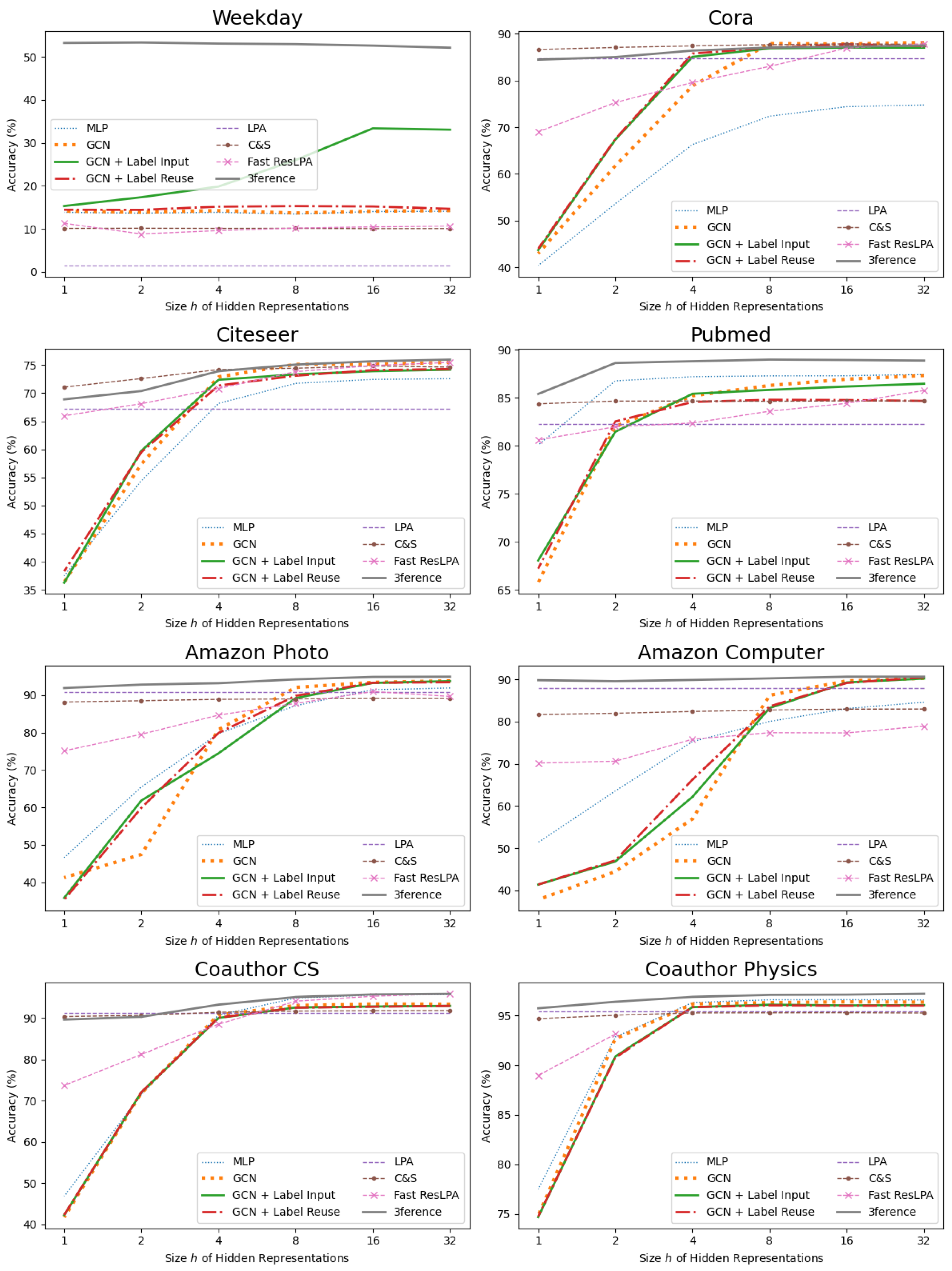
5.4.2. Number of Parameters

With different hidden representation sizes h, our implementations except the LPA have different amounts of learnable parameters. To study 3ference’s capability with different numbers of parameters, we experimented with different h and illustrate the results in Figure 5. Despite the result in Weekday Prediction, C&S, the Fast ResLPA, and 3ference outperformed the MLP and the GCN when the parameters were insufficient. This is because the former models inherit the ability of the LPA to utilize label information. This utilization simplifies the classification task dramatically, and it is free of learnable parameters. GCN + Label Input and GCN + Label Reuse also leverage label information. However, they need more parameters to capture the pattern of labels than 3ference because of the complexity of their networks. Therefore, they show no superiority to the MLP and the GCN on the number of parameters. This result suggests that structural information of labels can be beneficial to simplify tasks and is worthy of being taken into consideration when designing new Deep Learning methods.

5.4.3. Label Usage

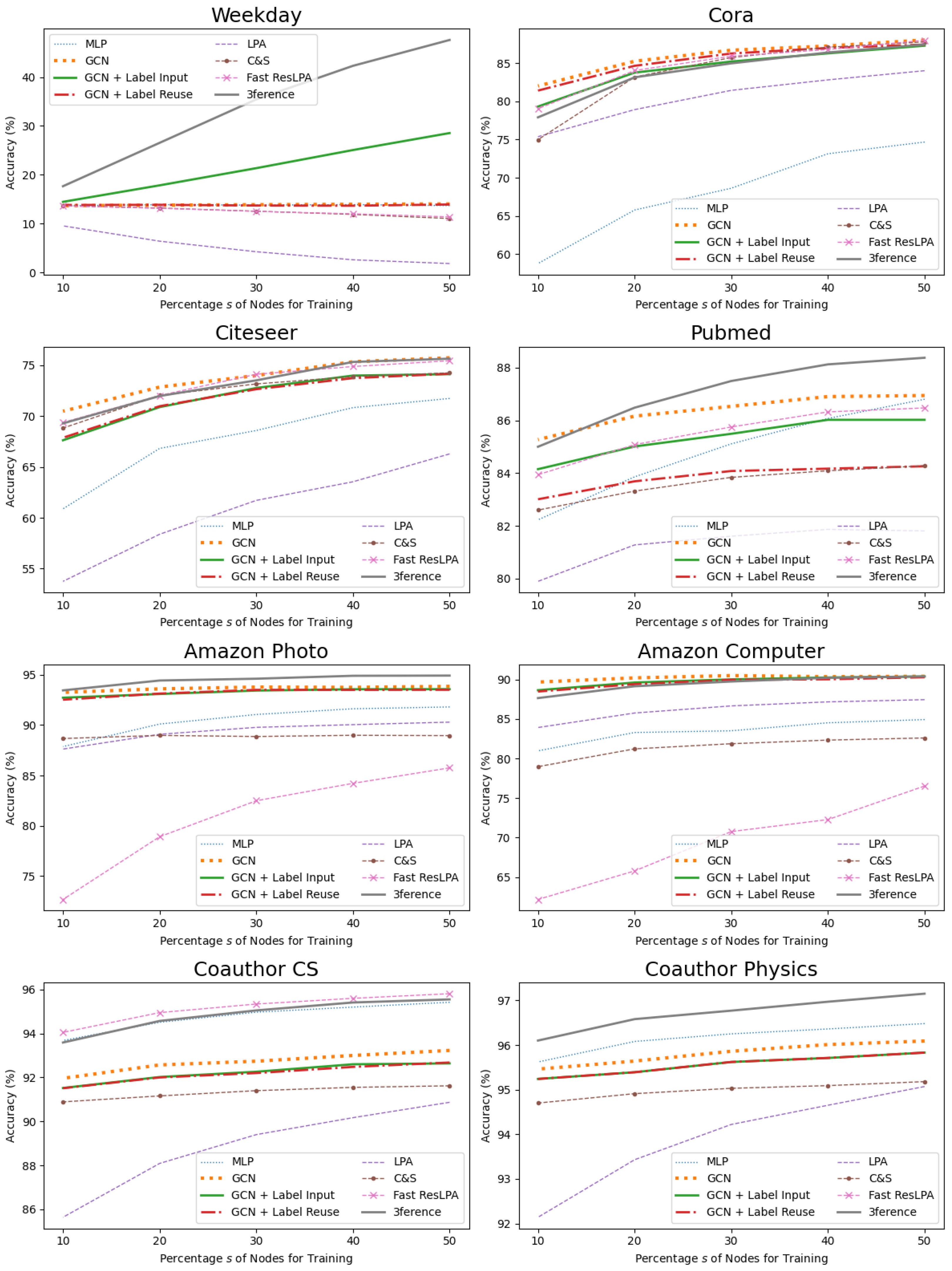
The proportion of labeled nodes in all nodes on a given graph may be crucial for LPA-based methods and 3ference. We experimented with different training sets that cover s percent of all nodes. The results are depicted in Figure 6. On almost all datasets, especially on Pubmed and Weekday Prediction, the curve of 3ference increases about twice as fast as that of GCN + Label Input. The reason behind this is that the Label Input trick has to divide the training set into two parts, causing a waste of resources. Compared against it, 3ference can capture more knowledge from the labels. This ability renders it able to achieve competitive performance with fewer known labels than other methods.

5.5. Analysis on the Label Transitions

In 3ference, we transform the referenced label $y_j$ by feeding it into the inference network instead of adding it to the approximated difference like the ResLPA. This is done for three purposes.

First, the input label distribution $y_j$ is a one-hot vector indicating which label the node $v_j$ is most likely to have. However, it cannot illustrate the associations among labels. For example, a horse is more similar to a donkey than a door. Therefore, in the label distribution of a horse, the value indicating the probability of the donkey label should be greater than that of the door label. A network with learnable weights can soften the hard distributions and learn such kinds of associations among labels.

Second, LPA-based methods rely on the assumption that adjacent nodes share similar or relevant labels. With the help of learnable weights, 3ference can still work when this assumption does not hold. If the labels of adjacent nodes are unrelated, 3ference can degenerate the transformation of $y_j$ into near-constant and focuses only on the central nodes’ feature information. If the labels of adjacent nodes are relevant, but not similar, the network can learn the transition pattern of labels between the referenced nodes and the central nodes.

Third, feeding $y_j$ into the network decouples the shape of the referenced labels $y_j$ and the predicting labels ${\widehat{y}}_i$. Therefore, 3ference also has the potential to be applied to heterogeneous graphs with different types of nodes.

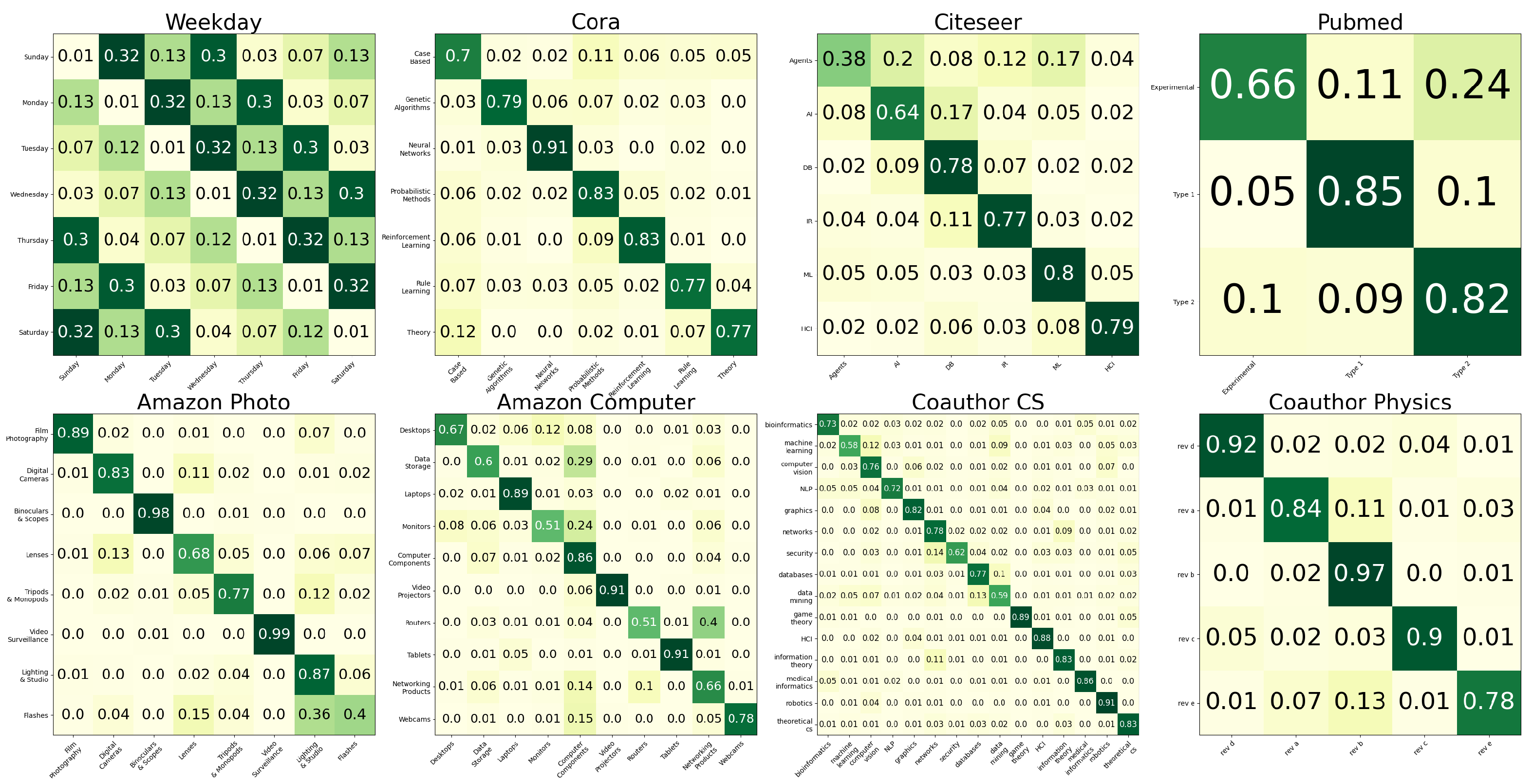
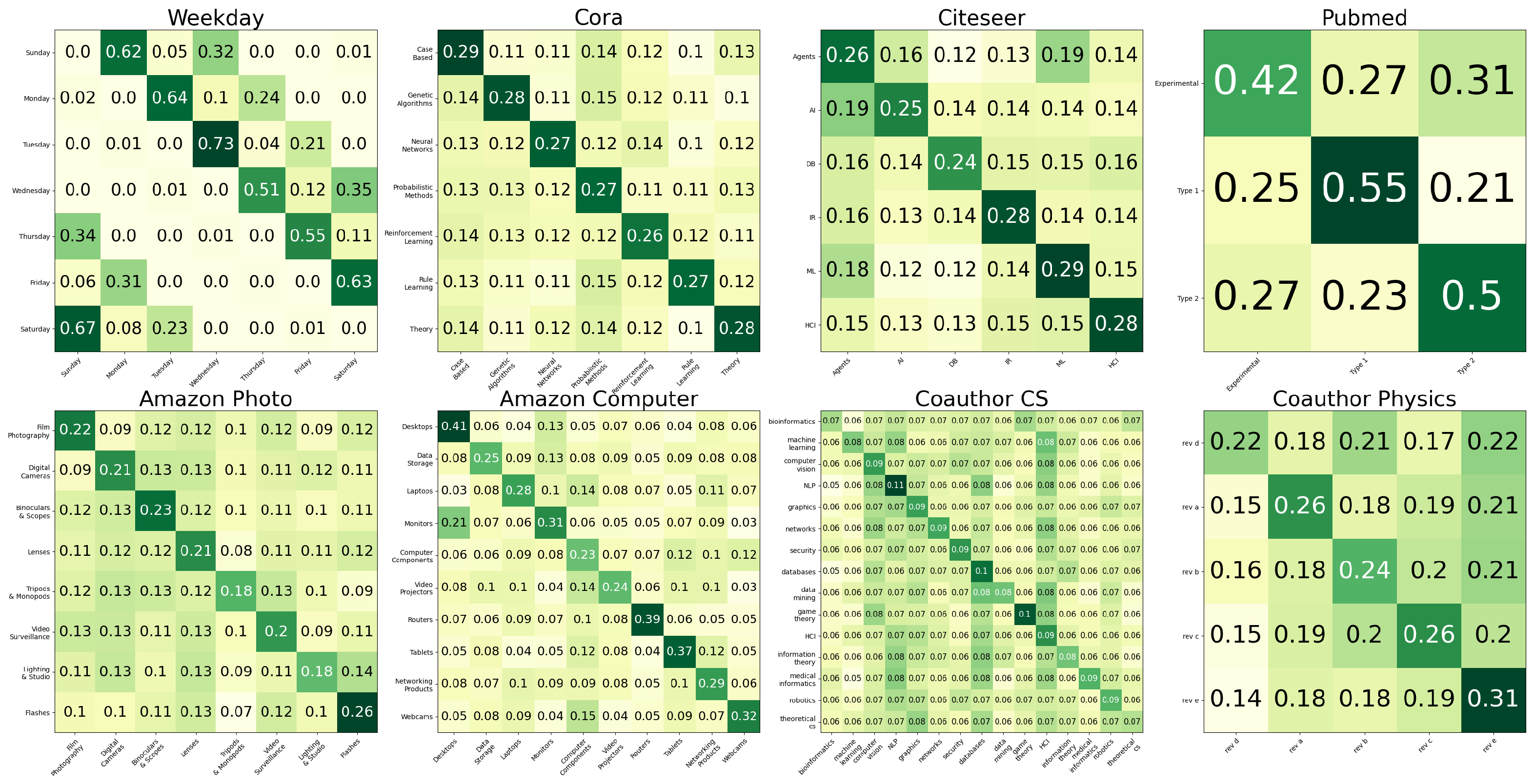
To examine the first two properties, we visualize the ground-truth label transition matrices (Figure 7) and the label transitions in a trained 3ference model (Figure 8). On Weekday Prediction, two matrices match well, suggesting that 3ference successfully gains the transition pattern of labels when labels of adjacent nodes are relevant, but not similar. On other real-world graphs, 3ference enlarges the elements along the diagonal lines in the learned label transition matrices because the adjacent nodes share similar labels. Specifically, while it can still achieve high accuracy scores, 3ference gains less label transition knowledge on the two co-authorship graphs than on other graphs. This is because, on such datasets where the feature information of the central nodes is sufficient, 3ference learns to focus more on features than on labels.

6. Conclusions

This work proposed to fully consider the structural information of both labels and features when learning on graphic data. Motivated by this idea, a method named 3ference was implemented to infer from references with differences. It inherits the ability of the LPA to predict accurately with much fewer parameters than GNN,s while overcoming the restriction of label patterns that the LPA and most GNNs suffer. The success of 3ference proves that the knowledge of label structures can help conventional Deep Learning methods simplify tasks, reduce the need for tagged labels, and apply to datasets with varying label patterns.

In the process of evaluating that method, this work proposes the Weekday Prediction task, which is easy for humans, but complicated for many Deep Learning methods. Such tasks are worthy of subsequent works to examine themselves. However, associating dates according to their Euclidean distances is not optimal to organize relevant dates. We think it is prominent to explore the methodology of finding relevant references for inferencing on both tabular data and graphic data in the future.

To keep this article refined and the networks in 3ference simple, we covered no topics about orthogonal techniques such as enhanced node features [29] and edge weights [4]. These techniques can be combined with 3ference to derive methods with more helpful characteristics in practice.