Article

Tuning of PID Control for the Double Integrator Plus Dead Time Model by Modified Real Dominant Pole and Performance Portrait Methods

1
Institute of Automotive Mechatronics, Faculty of Electrical Engineering and Information Technology, Slovak University of Technology in Bratislava, SK-812 19 Bratislava, Slovakia
2
Department of Computer Automation and Control, J. Stefan Institute, SI-1000 Ljubljana, Slovenia
*
Author to whom correspondence should be addressed.
Mathematics 2022, 10(6), 971; https://doi.org/10.3390/math10060971
Submission received: 16 December 2021 / Revised: 14 March 2022 / Accepted: 15 March 2022 / Published: 18 March 2022

Abstract

:
The paper discusses the proportional-integral-derivative (PID) controller from the viewpoint of (a) the analytical tuning of the PID controller for the double integrator plus dead time (DIPDT) model and (b) the numerical tuning using the performance portrait method (PPM). In the first case, the already published tuning with multiple real dominant pole, extended by integrated tuning procedures, which incorporate the inevitable low-pass filters by delay equivalences, is elaborated for modified sets of real poles. By considering several such modified sets of real poles, resulting in several new sets of controller parameters, the design can be better adapted to the requirements of the control tasks solved and to the limitations of the existing control loop hardware. In a noisy and uncertain environment, the balance between speed of setpoint and disturbance responses and acceptable excessive controller effort can thus be improved. The effectiveness of the analytical design can be evaluated using the numerical performance portrait method (PPM). For an already generated performance portrait (PP), it can offer a broad spectrum of controller settings that satisfy various design constraints. However, the results of the analytical design are still important as they facilitate the initial steps in the elaboration of the PPM and in explaining the nature of PID control. The developed controller tuning are compared using a new interpretation of PID controller as an extension of the stabilising PD controller by disturbance observer (DOB). The input disturbances reconstructed by DOB by evaluating the controller output of an integral process model in steady-state, can be estimated by a low-pass filter with a sufficiently long (integral) time constant. All analysed results are in full agreement with the proposed DOB interpretation, which furthermore contributes significantly to the explanation of the problems related to the optimal design of PID controllers.

1. Introduction

The approximation of input–output dynamics by a double integrator with transport delay is often used in the design of automatic control systems involving moving bodies as handled in motion control, power control systems, robotics, and so on. The pole assignment method is one of the most popular methods for designing simple systems [1]. Its advantage is that closed-loop requirements can be met simply by choosing a suitable pole configuration; however, the method is not suitable for the direct design of time-delayed systems [2,3,4,5,6,7,8]. This is because the transport delay is usually replaced by the Taylor or Padé expansion, which limits the pole placement method to a relatively narrow range of selected poles. We encounter similar limitations when using the popular SIMC (SIMple Control) tuning [9,10,11], which has been called “the best simple tuning in the world”; however, the gradually increasing demands on control performance in practice and the growing performance of hardware open up the possibility of developing control methods for processes with larger delays and unstable systems. A more detailed analysis of the SIMC method [12] has shown that its shortcoming lies in the approximation of delays and the evaluation of excessive controller effort with the total variation criterion (TV). The aforementioned works favour the use of the simplest controllers and are limited to stable systems, which results from both the nature of the model-based approach and the sensitivity constraints used in conjunction with the integral of absolute error ( I A E )-based optimisation. The values recommended in the textbooks for the maximum sensitivity M s [ 1.2 , 2 ] (which are suitable for the control of stable systems) cannot be applied to the control of unstable systems [13], where one even has to work with values ten times higher (e.g., [14] recommends M s 10 , [15] M s 20 ). Of course, the problems mentioned only occur in some special applications. For the majority of processes, the original or later modified SIMC approaches provide good control performance. This SIMC example can be used to illustrate the current overall situation in the field of PID control. It seems that a large number of existing methods [16] and a growing number of new methods (see e.g., [17,18,19,20,21,22,23], to name a few) seem to be looking for some important detail that has been overlooked so far in the abstraction process regarding the design of PID control, and they try to compensate for it by using different artificial intelligence methods or fractional-order PID control methods [24,25].
In this respect, the multiple real dominant pole (MRDP) method, which was used in the early days of control engineering [26,27,28,29], seems to be more conservative. Its analytical results remain valid over a wide range of time lags; however, its disadvantage is that it provides a single solution with an n-fold real dominant pole (where n is given by the characteristic quasi-polynomial order) and has no free parameter to adapt the solution to the variable requirements. When designing stable systems, the mentioned disadvantage can be eliminated by slowing down the transients with suitable low-pass filter, whose equivalent delay is added to the identified process delay. Such a solution also suppresses the adverse effects of measurement noise [30]; however, when controlling unstable systems, it may not be acceptable to increase the total delay by intensive filtering (see e.g., [31]). Moreover, the experimentally observed large differences in terms of the effects of noise and modelling imperfections that occur when proceeding from a stabilising PD to stabilising and disturbance-compensating PID controllers require a detailed analysis of the phenomenon.
In this paper, we show how the multiple real dominant pole method can be generalised for processes with several different sets of real poles to derive the corresponding sets of rigorously designed controller settings. The results of the analytical design are then additionally evaluated and compared with the numerical optimisation based on the performance portrait method (PPM). This two-stage analysis, based on a thorough comparison of optimal settings of PD and PID controllers, subsequently helps to explain the nature and purpose of series PID control as a particular type of plant stabilisation in conjunction with disturbance reconstruction and compensation. Series PI and PID controllers are among the oldest in history and among the most widely used controllers in the industry [32,33]. Despite several waves of innovation triggered by the state-space approach, internal model control, disturbance observer-based control, active disturbance rejection, etc., they remain in the focus of researchers and industrial users without deeper integration with newer techniques [34]. To fill this gap, in this paper we take a slightly different approach from the usual interpretation of PID controllers as three-term control, based on the work of Sperry and Minorsky from the beginning of the last century [33,35]. In addition to the special characteristics of series PID controllers in terms of limitations of control variables (which in parallel PID control leads to the emergence of the wind-up effect [36,37,38]), in this paper we focus mainly on the optimal tuning of PID controllers from the point of view of reconstruction and compensation of disturbances. PI and PID controllers can be represented, in accordance with modern and postmodern approaches, as including a disturbance observer (DOB) [39]. This is a very simple special form based on the evaluation of steady-state values of the controller output of integral models. Due to the nature of the DOB used, PID control includes a significant limitation in terms of choosing an appropriate integral time constant. In addition, the introduction of positive feedback to compensate for the reconstructed disturbances severely limits the possibilities for setting up the controller compared to the stabilising PD controller. The effectiveness and limitations of this particular DOB-based structure, based on the analysis of the obtained optimal settings, are discussed, which is the basic contribution of the paper.
The rest of the paper is structured as follows. Section 2 presents the performance measures used to evaluate the optimal PID controller design for the double integrator plus dead time (DIPDT) model. Section 3 starts with the optimal PD and PID controller tuning using the triple and quadruple real dominant pole (TRDP and QRDP) and extends this approach to several modified sets of four real poles (MFRP) in Section 4. The transients obtained with the proposed controllers, extended to include the inevitable implementation of noise reduction filters, are evaluated by simulation in Section 5. In Section 6, the analytical design of PID controllers is complemented, explained, and generalised by an analysis of their optimal settings using the performance portrait method. The results of the analytical and numerical design are discussed in Section 7 in the historical context of the development of PI and PID controllers as system stabilisation structures complemented by disturbance reconstruction and compensation using DOBs based on the evaluation of steady-state values of the controller output. All results of analytical and numerical tuning of PID controllers are compared with the proposed definition of the functional mission of PID controllers and fully confirm this proposal. The overall results of the article are summarised in in the conclusions.

2. Time and Shape Related Performance Measures

When evaluating the speed of transients, the integral of the absolute error ( I A E )
I A E = 0 e ( t ) d t ; e = w y ,
is used, where w denotes a piecewise constant reference setpoint, y the process output and e the control error. The advantage over using an alternative option called “settling time” [40,41] is that the I A E does not have to define the width of the zone around the desired state after which the transients are considered to be terminated. Since I A E minimisation of optimal responses typically leads to overshoot of the output, the shape-related constraints are combined based on the concept of monotonicity. The corresponding performance measures can be based on the total variation ( T V ), introduced in [10] as the sum of all absolute increments of a given variable. The fundamental problem with using T V to evaluate excessive control effort is that even changes in control action required to achieve the desired output transients after setpoint reference signal changes, or to eliminate disturbances count as the excessive control increments; therefore, some modifications must be made. Such T V modifications can then also be used much more broadly in evaluating the deviations of all loop transients from monotonicity.
These modifications include T V 0 ( y ) , using samples y i = y ( T s i ) , i [ 0 , ) of the output signal y ( t ) viewed with the sampling period T s , where
T V 0 ( y ) = i = 0 y i + 1 y i y y 0
T V 0 ( y ) can be interpreted as a measure of the deviation from monotonicity. T V 0 ( y ) = 0 only for monotonic responses y ( t ) . Otherwise T V 0 ( y ) > 0 . For a response with a single overshoot amplitude Δ , T V 0 ( y ) = 2 Δ .
For a response with a single pulse (1P) shape [41], i.e., a shape consisting of two monotonic intervals separated by an extreme point y m ( y 0 , y ) lying outside the interval formed by the initial and final output values y 0 and y , evaluating the deviations from monotonicity twice yields a deviation from an ideal 1P response
T V 1 ( y ) = i y i + 1 y i 2 y m y y 0
This performance measure is be used to evaluate disturbance step responses at the system output.
In the control of a double integrator [40,41], the shape of the ideal plant input (controller output) of a piecewise continuous control signal u ( t ) , t [ 0 , ) , which is required to obtain ideal monotonic setpoint steps and 1P disturbance steps of the output, is given by the inverse plant dynamics. It can be shown that it specified by two extreme points u m 1 , u m 2 , which occur at times t 1 , t 2 ( 0 , ) , lie between the initial and final values u 0 and u and satisfy the condition
( u m 1 u ) ( u m 2 u ) < 0 .
These extreme points divide the control signal into three monotonic control intervals. The excessive control effort, which represents the deviations from such a 2P response and summarises the deviations from monotonicity of the three subintervals, can be expressed as follows
T V 2 ( u ) = i u i + 1 u i 2 u m 1 2 u m 2 + ( u u 0 ) s i g n ( u m 1 u )
Another problem of transient optimisation and evaluation is the quantitative expression of the adequacy of the input effort for the achieved speed of the transients, which includes the optimality of the chosen parameters of the controller with respect to the system dynamics, design uncertainties, non-modelled dynamics, and measurement noise. However, the definition of adequacy cannot be easily generalised or standardised. Such a concept always depends on the given system and the requirements of a particular application. Since it is to be expected that as the transient speed increases, the excessive controller effort also increases, a combined (speed-effort) cost function
J k ( u ) = I A E k T V 2 ( u )
is considered for the optimisation of the controller settings. Here, the exponent k expresses a variable weighting of the speed of the transients with respect to the shape deviations considered, which is specified differently depending on the context of the optimisation.

3. PD and PID Controller Tuning with the MRDP Method

Let us consider the double integrator plus dead time (DIPDT) model [31]
F ( s ) = K s e T d s / s 2
With stabilisation by an ideal PD controller
U ( s ) = ( K p + K d s ) E ( s )
the closed loop transfer function
F w y ( s ) = Y ( s ) W ( s ) = K s ( K d s + K p ) e T d s s 2 + K s ( K p + K d s )
has a characteristic quasi-polynomial
A P D ( s ) = e T d s s 2 + K s ( K p + K d s )
It is well known that the change in the nature of transients from exponential to oscillatory occurs at multiple real poles of the system. To find such an “optimal” pole s o and two parameters of the controller K p o , K d o , we need three equations that give the required multiplicity of the pole s o to make the calculation possible. From the properties of the triple pole, the parameters were calculated to meet the following requirements:
A P D ( s ) ; d A P D s d s ; d A P D 2 s d s 2 s = s o = 0
In solving the given relations, we are interested in s o , which is closest to the imaginary axis in the left half-plane and which we can call the dominant pole. From the second derivative
d A P D 2 s d s 2 = ( s 2 + 4 s + 2 ) e T d s = 0
we obtain an equation solvable via the variable s, which gives the TRDP and the associated time constant as:
s o = ϵ / T d = 0.5858 / T d ; T o = 1 / s o = 1.7071 T d
The fastest non-oscillatory responses then correspond to a triple-real-dominant-pole (TRDP) tuning
K p o = e ϵ ( 10 2 14 ) K s T d 2 = 0.079 K s T d 2 ; K d o = ϵ e ϵ K s T d = 0.461 K s T d ; ϵ = 2 2
A more compact notation of obtained results yields dimensionless controller parameters
κ o = K p o K s T d 2 = 0.079 ; δ o = K d o K s T d = 0.461 ; τ D = δ o / κ o = 5.8284 ; p o = s o T d = 0.5858 .
To eliminate the overshoot of the setpoint step responses caused by the zeros of F w y in (9), a pre-filter must be added to the PD controller (8)
F p ( s ) = 1 + b s 1 + T D s ; T D = K d K p ; b = T o ,
where both the numerator zero 1 / T D and one of the triple poles of the closed-loop s o = 1 / T o are cancelled. For unit setpoint step responses, the controller then delivers the I A E value
I A E w = 4.1213 T d .
Similarly, the following applied to an ideal parallel PID controller
C ( s ) = U ( s ) E ( s ) = K c 1 + 1 s T i + s T D = K c + K d s + K i s
where K c is the controller gain, T i the integral and T D the derivative time constant, we obtain the closed-loop transfer functions
F w y ( s ) = Y ( s ) W ( s ) = K c K s ( 1 + T i s + T i T D s 2 ) T i s 3 e T d s + K c K s ( 1 + T i s + T i T D s 2 ) F i y ( s ) = Y ( s ) D i ( s ) = K s T i s T i s 3 e T d s + K c K s ( 1 + T i s + T i T D s 2 )
For the characteristic quasi-polynomial
P ( s ) = T i s 3 e T d s + K c K s ( 1 + T i s + T i T D s 2 )
the number of unknown parameters now requires consideration of four equations. These can be formulated as conditions for the quadruple real dominant pole (QRDP) (11)
P ( s ) ; d P s d s ; d P 2 s d s 2 ; d 3 P s d s 3 s = s o = 0
By solving these, one obtains the dimensionless (normalised) controller parameters
κ o = K c o K s T d 2 = 0.1248 ; δ o = K d o K s T d = 0.5045 ; η o = K i o K s T d = 0.0121 τ i o = T i o / T d = 10.324 ; τ D o = T D o / T d = 4.043
They correspond to the dimensionless dominant pole/time constant
p o = s o T d = 0.416 ; τ o = 1 / p o = 2.405
To avoid overshooting of the setpoint step responses due to zeros of F w y in (19), the derived PID controller (18) can be extended by a pre-filter
F p ( s ) = 1 + b s + c s 2 1 + T i s ( 1 + T D s )
Since the simplest numerator tuning with the values
b 0 = c 0 = 0
further slows down the setpoint response, we will consider numerator tuning that speeds up the setpoint responses by cancelling one or two of the dominant poles s o , or s o 2 , when (with using the number of cancelled poles as index)
c 1 = 0 , b 1 = T o , or c 2 = T o 2 , b 2 = 2 T o ; T o = 1 / s o = 2.405 T d
Depending on the numerator order, the QRDP tuning yields I A E values
I A E w 0 = 10.323 T d ; I A E w 1 = 7.918 T d ; I A E w 2 = 5.513 T d ; I A E i = 82.728 T d 3 .
The first two controller parameters K c and K d can be compared with the corresponding values of the PD controller, which shows the basic problems of building PID controllers with the QRDP method.
Remark 1
(Basic paradoxes in building PID controllers with the QRDP method). Due to the introduction of the I-action implemented in form of a positive feedback, the proportional gain of the PID controller has to be increased by 0.1248 / 0.079 = 1.58 times and the derivative gain by 0.5045 / 0.461 = 1.1 times. Nonetheless, the speed of the transients decreased by 0.586 / 0.416 = 1.4 times with respect to the dominant poles and with respect to I A E w , in the optimal case given by I A E w 2 by 5.513 / 4.1213 = 1.34 times, 1.92 times for I A E w 1 , and by 2.5 times for I A E w 0 . This velocity decrease, together with the increased sensitivity of the control loop, may be sufficient to completely eliminate the advantages of the controller I-action (as experimentally confirmed in [31]).
Therefore, in the following we focus on alternative circuit settings that, while retaining the advantages of rigorous tuning, would mitigate the above shortcomings and thus help to the expand the possible applications of this method in practice.
Remark 2
(QRDP PID controller integration time constant). The integration time constant of the QRDP PID controller T i = 10.324 T d is much larger than the dominant time constant T o = 1.707 T d of transients stabilised by the TRDP PD controller. This means that the signal at the output of the low-pass filter with the time constant T i settles much later than the output of the stabilising PD controller (14).

4. Modified Controller Tuning

4.1. Tuning of the PID Controller According to a Modified Position of One Real Pole

Next, find a controller tuning that corresponds to a triple real pole s o and a single pole s o / m , where m > 0 is a real positive number. To simplify the solution, we start with a characteristic quasi-polynomial
P ( p ) = τ i p 3 e p + κ ( 1 + τ i p + τ i τ D p 2 ) ; p = T d s
For a chosen m, the corresponding set of poles must satisfy four conditions
P ( p ) ; d P p d p ; d P 2 p d p 2 ; p = p o = 0 ; P ( p o m ) = 0 ; m > 0
From
e p o / m = κ ( 1 + τ i p + τ i τ D p 2 ) τ i p 3 p = p o / m
it is possible to express
e p o = κ ( 1 + τ i p + τ i τ D p 2 ) τ i p 3 p = p o / m m
and insert e p o into the first three Equation (29). If one solves these systems of equations as a function of κ , τ D , τ i and inserts this solution, parameterised by p o , into (30), one obtains an equation of the form
e p o = f ( p o )
with a single unknown p o . The solutions obtained with computer algebra are listed in Table 1 for different values of the parameter m.

4.2. Tuning the PID Controller According to a Modified Position of Pair of Poles

Larger effects of changes can be expected for a controller tuning corresponding to a obtained double real pole s o and a changed pole pair s o / m , where m > 0 is a real positive number. A characteristic quasi-polynomial (28) is again assumed to derive the simplified solution. The chosen set of poles leads to four conditions
P ( p ) ; d P p d p p = p o = 0 ; P ( p ) ; d P p d p p = p o / m = 0 ; m > 0
From
e p o / m = κ ( 1 + 2 τ D p ) p 3 + 3 p 2 p = p o / m
it is possible to convert
e p o = κ ( 1 + 2 τ D p ) p 3 + 3 p 2 p = p o / m m
and e p o into the first two equations (33). Solving these systems of equations in terms of κ , τ D , τ i and inserting this solution parameterised by p o into (34), one obtains an equation of the form
e p o = f 2 ( p o )
with a single unknown p o . The solutions obtained with computer algebra are listed in Table 2 for different values of the parameter m.

4.3. Tuning PID Controller According to Threefold Change in Pole Position

The strongest effect of changes can be expected for a controller tuning corresponding to a single obtained real pole s o and a modified triple pole s o / m , where m > 0 is a real positive number. Starting from the characteristic quasi-polynomial (28), the chosen set of poles yields four conditions
P ( p o ) = 0 ; P ( p ) ; d P p d p ; d P 2 p d p 2 ; p = p o / m = 0 ; m > 0
The solutions obtained using computer algebra are listed in Table 3 for different values of the parameter m.
For all modified controllers, the prefilter tuning can be derived to cancel a dominant pole s o , s o / m , or a pole pair s o 2 , ( s o / m ) 2 , or s o 2 / m
c = 0 , b = T o , or c = 0 , b = m T o ; T o = 1 / s o .
Remark 3
(Integration time constants of modified PID controllers). Note that Remark 2 also applies to all modified PID controllers listed in Table 1, Table 2 and Table 3.

4.4. Tuning the Controller with Equivalent Delay

To obtain a proper controller transfer function, which is necessary for its implementation, and to attenuate the measurement noise, the ideal controller (18) must be combined with a binomial low-pass filter Q n ( s )
Q n s = 1 T f s + 1 n ; n 1
In order to ensure sufficient filtering, the sampling period T s must be chosen so that the following condition is fulfilled T s < < T f .
The model dead time T d must include, in addition to an estimate of the loop delay T m (which is the sum of the delays of the process, the actuators and the measurement sensors with a communication and computation delay), an intentionally introduced equivalent filter delay estimate T e
T d = T m + T e
Here T e (see e.g., [30]) is used to approximate the dynamics of the low-pass filters Q n ( s ) in terms of a dead time that can simply be added to the total dead time T d . T e can be approximated as follows
T e = n N T f
where the coefficient N can be given by values in the range from N = 0.5 (equivalence based on “the half rule”) to N = 1 (equivalence based on “the average residence time”).
Examples of setpoint and disturbance step responses with pole configurations and tunings according to Table 1, Table 2 and Table 3 are shown in Figure 1, Figure 2 and Figure 3. For the dead time of the system, denoted by T m = 1 , all these responses take into account the first-order implementation filter (39) with time constant T f = T m / 10 , which is included in the controller tuning according to (41) with N = n = 1 . They prove that the smooth, almost ideal transients given by the QRDP method can also be extended to wider configurations of real closed-loop poles. While the effect of increasing m in terms of the resulting circuit dynamics is always clear (increasing m slows down the disturbance responses), the resulting effect in terms of setpoint responses also depends on the prefilter setting used. Looking at the change in a single pole by removing it from the setpoint response, an increase in m can actually speed up the setpoint responses.
A picture of the effects of setting changes on the open-loop Nyquist curves can be obtained from Figure 4.

5. Evaluation of the Performance Offered by the Analytical Design

The above conclusions are best quantified using appropriate performance measures. The effect of increasing m on the I A E d values, corresponding to a step change in input disturbance, is significantly greater when the two modified poles are considered (see Figure 5 and Figure 6, or the numerical values in Table 4). With the setpoint responses, the role of the appropriate prefilter setting also becomes apparent.
To evaluate the influence of noise on the resulting loop performance, a noise generator was added to the Matlab/Simulink scheme (see Figure 7), represented by the Uniform Random Number block with output amplitude | δ n | < 0.01 . The influence of the noise on the output signals was practically negligible, but became strongly apparent at the controller output, where the noise amplitudes completely covered the useful signal.
The I A E and T V 2 ( u ) values measured with sampling period T s = 0.001 and simulation time t s i m = 50 s, corresponding to the PID control with prefilter (24) and a first-order implementation filter calculated according to (41) with a double real pole p o and a pole pair p o / m according to Table 2 for the loop with T m = 1 ; K s = 1 ; T f = T e = 0.1 ; n = N = 1 , are shown in Figure 8 (for the numerical values see Table 5). While the I A E values increase with increasing m, the excessive controller effort values decrease. To automate the selection of the optimal solution in such a situation, it is necessary to introduce cost functions (6) that take both trends into account in an appropriate way. The key moment for the design of such a function is the choice of the appropriate weighting, where the coefficient k is chosen according to the specifications of the particular application. As the curves in Figure 9 show, for a value of k = 1 the increasing trend J 1 with increasing m predominates, but for a lower weighting of the control speed ( I A E values), given by k = 1 / 10 , the general decrease in the cost function already prevails.

Comparing the PD and PID Controllers

Let us return to the basic problem of the transition from a stabilising PD controller to a PID controller that allows full compensation after piecewise constant input disturbances from Remark 1. Now repeat the experiment from the above evaluation of different modifications of the PID controller (see Table 6), keeping all parameters and settings of the implementation filter for the PD controller. Under the influence of noise we obtain the following values:
I A E w , P D = 4.533 ; T V 2 , P D ( u w ) = 560.3106
Comparing the figures (42) with the values of the PID controller in Table 6, we see that despite the improvements achieved by the changes, the ratio of transient speed to excessive controller effort has not improved significantly. Of course, additional sets of real poles on which the design is based could also be investigated; however, since at the time corresponding to the value T o , the mode value corresponding to the time constant 4 T o is practically zero, one can assume that the ratio m = 4 already covers all realistic combinations of real poles with sufficient accuracy.

6. Analytical Tuning versus Performance Portrait Method

In the following, we compare the results of the analytical tuning of the controllers based on sets of real dominant poles with the performance portrait method (PPM). PPM [40,41] assumes verification of loop properties at all possible relevant controller settings, which should be expressed by a grid of points whose spacing is chosen fine enough to capture all loop properties of interest. We simulated the loop (or control the process in real time) over this grid and store the obtained transient properties in a matrix of performance measures. These simulations should capture all the important features of the plant’s behaviour. Given the multi-point loop evaluation, the authors of [42] referred to this method as a “brute force” approach; however, this statement is not entirely accurate, because:
  • PPM is the only optimisation method that, once a performance portrait (PP) has been generated in dimensionless variables, allows its easy and unlimited reuse for different circuit parameters and criteria to select the optimal solution in different combinations.
  • Has no problems with convergence to the optimal solution, if the scope of PP generation and the point grid have been determined appropriately.
  • The success of the method depends primarily on the choice of appropriate performance measures that can overcome the effectiveness of traditional constraints based on maximum sensitivity ( M s ).
  • Similar methods for evaluating all relevant (admissible) solutions and selecting the best solution are often applied in other areas of social practice, not only to mention public procurement as a possible example.

6.1. Parallel PID Tuning without Prefilter Optimisation

The first step in using PPM is to select the appropriate ranges of each parameter when dealing with the PID controller settings for the DIPDT system. In this step we rely on the results of analytical controller design from previous sections, where we found optimal solutions with parameters the (22) and with the parameters in Table 1, Table 2 and Table 3, which define the intervals of interest as κ o [ 0.079 , 0.125 ] ; δ o [ 0.45 , 0.51 ] ; τ i o [ 10 , 15 ] ; τ D o [ 4 , 5.83 ] (or τ i o [ 10 , ] , if one also wants to include the PD control). In view of these values and the need to examine their immediate surroundings, we have therefore opted for PP with the ranges
κ [ 0.05 , 0.35 ] ; Δ κ = 0.01 ; δ [ 0.35 , 1.05 ] ; Δ δ = 0.1 ; τ i [ 6 , 22 ] ; Δ τ i = 2 .
If we want to generate PP independently of the choice of filter needed to implement the derivative action of the PID controller, we can use a scheme with available output derivative (Figure 10). In this case, however, the prefilter must be chosen as follows to delete the zero of F w y ( s )
F p ( s ) = b T i s + 1 T i s + 1
To avoid choosing the optimal setting of the prefilter numerator chosen as b T i s + 1 , b ( 0 , 1 ) (which would require increasing the size of PP), we choose the default value b = 0 , which partially slows down the setpoint responses.
When generating PP, we simulated the transients corresponding to the unit setpoint steps and the unit input disturbance steps. After evaluating them, we stored the values I A E w , I A E d , T V 2 ( u w ) , T V 2 ( u d ) , T V 0 ( y w ) , T V 1 ( y d ) in the performance measures matrix.
After creating PP, we started comparing the results from PPM obtained with the analytical design. We first focused on the fastest possible transients with the smallest possible total values
I A E = I A E w + I A E d T V 2 ( u ) = T V 2 ( u w ) + T V 2 ( u d )
taking into account equal weighting on the results from the evaluation of the unit setpoint and disturbance step responses. With regard to the I A E values (27), this means that in the search for the optimal PID parameters, the values corresponding to the disturbance step responses will dominate. As for the deviations from the ideal transients, we have chosen separately
T V 2 ( u w ) 0.1 ; T V 2 ( u d ) 0.1 ; T V 0 ( y w ) 0.01 ; T V 1 ( y d ) 0.01 .
Searching over the calculated and stored PP with performance measures that satisfy the above requirements yields optimal controller tuning
κ o = 0.24 ; δ o = 0.70 ; τ i o = 8 .
A comparison of the transients with the analytical tuning in Figure 11 shows that PPM makes it possible to find transients similarly fast as with the QRDP method even without the prefilter optimisation. The advantage of the QRDP setting, however, is that it works with lower controller gains (which is important for noisy control loops). It should provide ideal response shapes for all values of the model parameters K s and T d . The non-zero shape deviations entered for dimensionless quantities are subject to changes depending on the model parameters during the transition to real values of the shape deviations, which means that they can ultimately be significantly different [41]. This transformation must be taken into account when specifying the search conditions.
From the limited area with T V 1 ( y d ) 0.01 in Figure 12, which satisfies all specifications (46) at τ i = 8 , it is obvious why it is not possible to significantly reduce the noise effect by reducing the proportional and derivative gains κ and δ . The shape of this area does not allow a significant shift of the operating point without violating the specifications.
However, if we find the optimal operating point corresponding to a reduced value δ = 0.35 (see Figure 13), we calculate the optimal setting as
κ o = 0.08 ; δ o = 0.35 ; τ i o = 14 .
We see that reducing the derivative gain also leads to a reduction in the proportional gain and an increase in T i . If we needed to reduce the gains further, it would be necessary to generate PP for lower δ values and possibly adjust the ranges of other PP variables. Similarly, it would also be possible to extend the range of performance measures, considered, for example, by looking for disturbance responses with limited maximum output amplitude.

6.2. Alternative Controller Tuning Optimised under Consideration of Sensitivity Constraints

To complete the comparison, the responses with PID controller optimised under M s constraints (see Table 2 in [11] ) are going to be used. The dimensionless parameters of the series PID controller for three M s values are considered
κ = 0.0354 ; δ = 0.382 ; τ = 10.74 ; M s = 1.59 κ = 0.0505 ; δ = 0.4737 ; τ = 9.37 ; M s = 1.80 κ = 0.0625 ; δ = 0.5475 ; τ = 8.64 ; M s = 2.00
They can be recalculated for the parallel controller according to (52) as follows
κ o = 0.0710 ; δ o = 0.1905 ; τ i o = 21.5310 ; M s = 1.59 κ o = 0.1011 ; δ o = 0.2367 ; τ i o = 18.7502 ; M s = 1.80 κ o = 0.1259 ; δ o = 0.2719 ; τ i o = 17.4000 ; M s = 2.00
For simplicity, we again use the prefilter (24) with the numerator parameters b = c = 0 . The corresponding transients in Figure 11 show these responses yet much slower than for the QRDP and PPM tuning. The question naturally arises whether their speed, such as the speed corresponding to the PPM setting, does not carry risks in terms of lower robustness.
A similar task for the integrator plus dead time (IPDT) system analysed in [41] has shown that PPM can solve a robust design with uncertain values of model parameters specified in intervals much more efficiently than sensitivity-constrained optimisation.
The fundamental limitation here remains the visualisation of the information contained in the multidimensional PP, which by its nature is more suitable for computer support than traditional texts.
The whole issue can be illustrated by plotting a three-dimensional (3D) PP cross-section for the optimal value of τ i = 8 (Figure 12). We see that the optimal point found, which satisfies the given shape constraints for input and output (46), lies within the defined areas and its localisation is predominantly influenced by the admissible values of T V 2 ( u d ) .
Similarly, we were able to show that when the integration time constant τ i is reduced to speed up the responses, the admissible areas corresponding to the constraints on T V 0 ( y w ) and T V 1 ( y d ) disappear, so that we no longer find the optimal setting that satisfies the given shape requirements (46).
So far, we have shown with the help of PPM that in the analytical design of the regulator considering different MFRPs, we did not omit any settings at which the resulting dynamics could be significantly improved, especially in terms of T i reduction. This statement will not change even after the PPM has been extended to optimise pre-filter settings [43]; however, a complete picture of the usefulness of the calculated PID controller setting can only be obtained by evaluating the effect of the noise. If we again use noise generation by the Uniform Random Number block with an amplitude of δ n 0.01 , we obtain the performance measures in Figure 14 calculated according to (6) and (45). Evaluation of the setpoint step responses shows that the optimal tuning (47) found by PPM yields almost the same I A E w as the QRDP tuning. However, since we used PP without optimised prefilter tuning, which is achieved with higher controller gains (47), the corresponding T V 2 ( u w ) values are higher than for the QRDP tuning (22) with the prefilter cancelling one closed-loop pole (26). The same is true for the combined cost function (6) J k ( u w ) et for the setpoint responses.
Tuning (48) with reduced controller gains determined via PPM results in a significantly higher I A E w and a lower value of T V 2 ( u w ) . While the cost function J 1 ( u w ) with a higher weighting of transient speed for PPM shows almost the same values as the QRDP tuning, the cost function J 0.5 ( u w ) corresponding to a lower weighting of the transient speed shows better performance.
All I A E -optimisation-based PID settings with M s constraints yield the highest I A E w values and lower T V 2 ( u w ) values than the QRDP method. While they are comparable to the other design methods when evaluated with J 0.5 ( u w ) , they are significantly worse when evaluated with the cost function J 1 ( u w ) , which gives higher priority to the speed of the transients.
Similar conclusions can be drawn for the summary performance measures (45) and (6). The differences in I A E values are not as large as for I A E w , which consequently also affects the combined cost functions (6) for k = 1 and k = 5 . While much attention has been paid to considering Pareto fronts in terms of setpoint and disturbance responses when designing optimal PID controller settings, a similar evaluation of transient rate and noise sensitivity is not yet known.
The knowledge gained could be extended to larger values of T i , which are of interest to us with respect tof the transition from PID control to PD control considering T i .
Remark 4
(Validation of Remarks 2 and 3). Also the PP-based analysis of transients satisfying shape-related constraints (46) confirms the property resulting from Remarks 2 and 3 that the value of T i cannot be arbitrarily reduced to accelerate the reconstruction of the disturbances and the speed of the transients.

7. PID Controllers as Stabilising Controllers with Disturbance Observer (DOB)

The use of PPM, which allows us to overcome the computational difficulties of analytical design, has not produced significant changes in transients; therefore, we try to look at the problem of optimal setting of PID controllers from a broader perspective and include other alternative approaches. Although PID controllers are very commonly used for disturbance compensation, their evaluation and comparison with other alternative methods of reconstruction and disturbance compensation, such as the “modern” state-space approach [44,45],“postmodern” disturbance observer (DOB) based control [46], active disturbance rejection control (ADRC) [34,47], or intelligent PID control (referred to as model-free control) [48], is still pending.

A Brief History of Series and Parallel PID Control

In explaining the fundamental problem of the transition from PD to PID control, which causes the large increase in sensitivity to measurement noise and a significant decrease in the speed of transient responses experimentally demonstrated in [31], we must first understand the associated change in the functionality of the PID controller, in which the ability to eliminate the effects of constant disturbances plays a key role. The study of the effectiveness of automatic control with disturbance compensation has been the subject of intense research for decades [34,45].
At the beginning of 20th century, two branches of automatic process control development emerged. The first was more practically oriented, the second investigated the theoretical aspects of automatic control. One of the pioneers of PID controllers is Elmer Sperry, who as early as 1911 developed an autopilot for ships and aircraft, attempting to imitate the behaviour of a human operator. The theoretical analysis of effective automatic control of ships was carried out in 1922 by Nicolas Minorsky, whose research also based on an analysis of the activities of the human operator, which he converted into mathematical operations and justified the need for proportional, integral and derivative actions of the controller [35]; however, the problem did not end with the naming of the necessary components, but rather overshadowed the need to divide the two levels of the proposal: stabilisation of the basic system and counteracting of disturbances involving deviations from the basic system [34].
First of all, it should be recalled that the first PI controllers, which appeared in 1935–1938 as the pneumatic regulators “Fulscope” (by Taylor Instrument Companies, originally called “pre-act”) and “Stabilog” (by Foxboro Instrument, known as “Hyper-reset”, [49]) played an important role. They arose from the generalisation of older controllers called “automatic reset”, in which the output of a stabilising P controller was changed by introducing a positive feedback via a delay with the time constant T i 
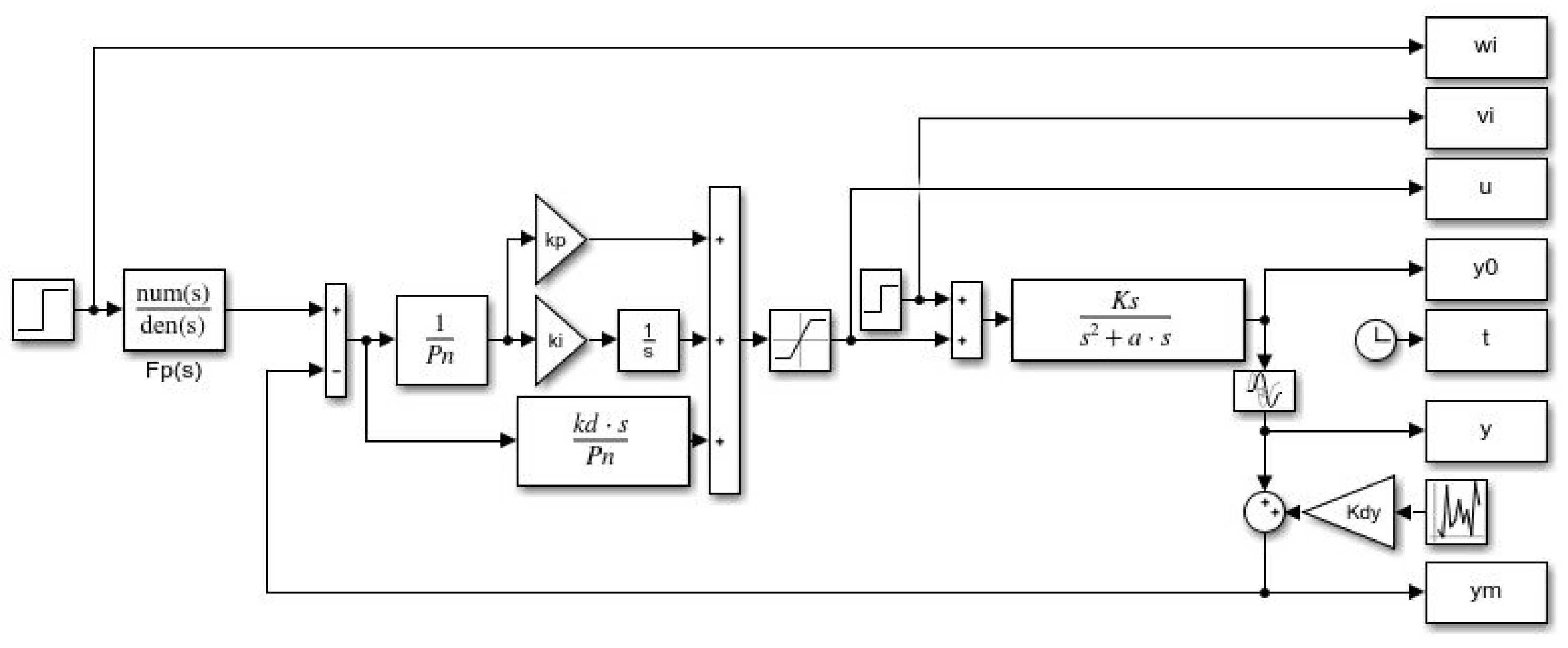
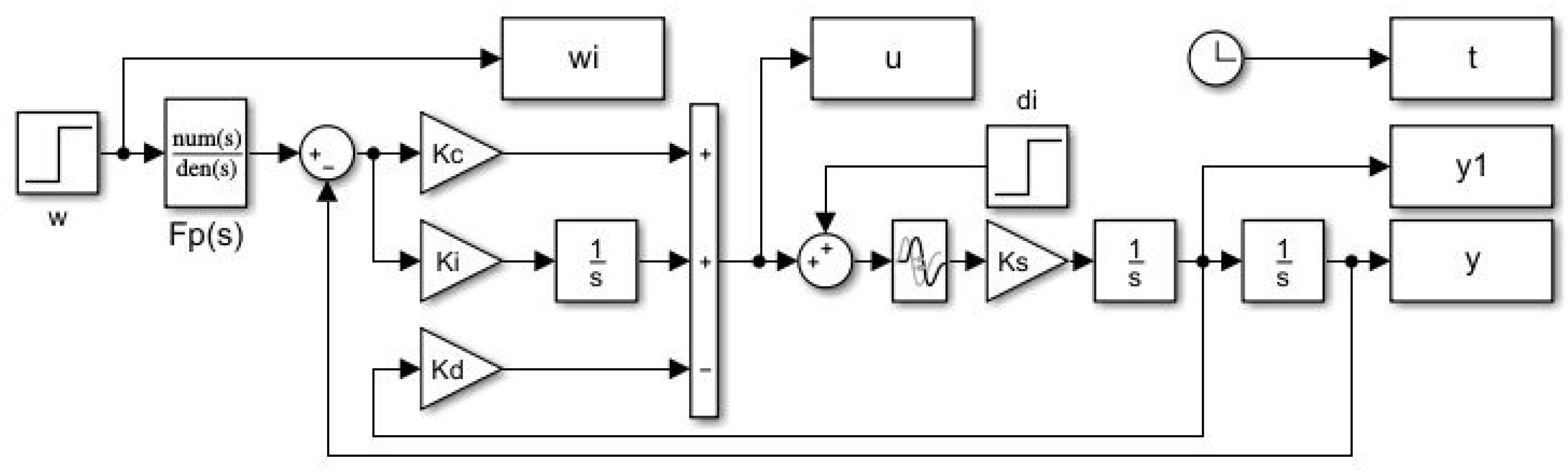
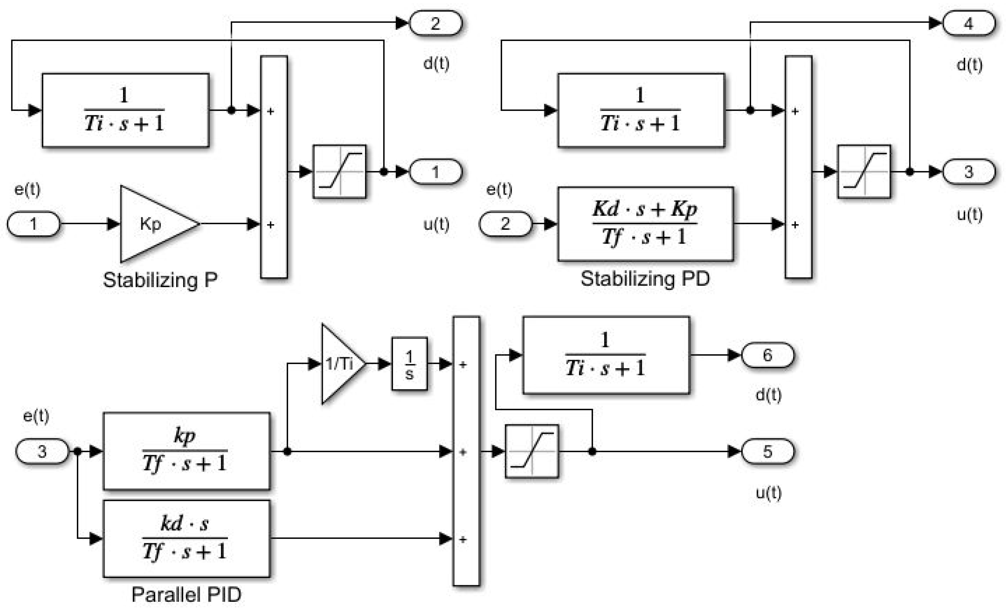
. Its operation can be easily explained using the example of the control of integrating systems, where the input of the integrator must be zero in steady state. This means that the controller output in steady state must be equal to the negative value of a constant input disturbance. Thus, to reconstruct and compensate the disturbance, it is sufficient to wait until the next steady-state reached with a stabilising controller (P or PD), and then subtract the obtained disturbance value from the previous output of the stabilising controller. In view of the opposite signs of the steady-state controller output and the reconstructed disturbance and the need to compensate for the disturbance by subtracting it from the controller output, this means adding the value of the steady-state control signal to the controller output. Such a procedure means the introduction of positive feedback. If one wants to avoid the necessity of a steady state testing, it is sufficient to introduce such a feedback with a sufficiently long delay T i , which is significantly longer than the dominant time constant of the stabilised loop transients (see Figure 15).
In the later development of the theory of automatic control, the use of the older (and possibly more concise) terminology was abandoned and new names for the series PI and PID controllers were introduced instead. Although the structure of series PI and PID controller can be found in numerous textbooks, its characteristic as a stabilising controller supplemented by a disturbance observer went unnoticed. The companies that developed series PID controllers were not motivated to explain its essence, but rather sought patent protection for their solutions, which are determined by aspects other than the explanation of functionality. The theoretical “branch” was content with naming the components that the PID controller introduces into to the circuit and their secondary effect on the achieved performance as the primary mission of the controller. Even if an attempt is made to present PID controllers as an industry standard, this is not possible due to the existence of various controller structures, of which the best known are series and parallel controllers. Let us just remember that in order to achieve the same loop dynamics (to obtain the same controller transfer function), it is generally necessary to calculate different series and parallel PID parameters, when (using the indices “s” and “p”) it must be true that
C ( s ) = U ( s ) E ( s ) = K c s ( 1 + s T i s ) ( 1 + T D s s ) s T i s = K c p 1 + T i p s + T i p T D p s 2 T i p s
The transitions from a series to a parallel controller is always possible according to
T i p = T i s + T D s ; K c p = K c s T i s + T D s T i s ; T D p = T i s T D s T i s + T D s
The calculation of the series PID parameters from the parallel PID controller according to
T i s = [ T i p ± ( T i p 2 4 T i p T D p ) ] / 2 K c s = K c p [ T i p ± ( T i p 2 4 T i p T D p ) ] / ( 2 T i p ) = = K c p [ 0.5 ± ( 0.25 T D p / T i p ) ] T D s = [ T i p ( T i p 2 4 T i p T D p ) ] / 2
is only possible for T i p 4 T D p .
When designing controllers, we should not forget the fundamental aspects of control design. Just as “every good regulator of a system must be a model of that system” [50], it should also be true “if the controller is to compensate for disturbances, it must also reconstruct them”. In the case of PID controllers used with piecewise constant input disturbances, this can be verified by calculating the transfer function
F i u ( s ) = U ( s ) D i ( s ) = F ( s ) C ( s ) 1 + F ( s ) C ( s ) = K c K s ( 1 + T i s + T i T D s 2 ) T i s 3 e T d s + K c K s ( 1 + T i s + T i T D s 2 )
In steady state, with F i u ( 0 ) = 1 , compensation of a constant input disturbance d i is provided by the controller output.
Since the mission of the series PID controller is also crucial for the successful solution of its optimal settings, we summarise it in the following definition.
Definition 1
(Series PI and PID controllers). The series PI and PID controllers are the first historically known disturbance counteracting controllers using DOB that complement the stabilising P and PD controllers by the positive feedback of their output. They can be designed by approximating the steady-state output values of the controller based on integral models, representing the negative values of constant input disturbances. To filter out stabilising transients, the (nearly) steady-state values of the controller output can be achieved using low-pass filters with sufficiently long (integral) time constant T i .
Remark 5
(Compactness of the series PID controller). The reconstructed disturbance signal could also be obtained (see Figure 15) by observing the output of the parallel PID controller through a delay with a sufficiently long time constant T i (to filter out stabilising transients), but (in contrast to compact series PID controllers), such an observer would require an additional filter transfer function. Furthermore, the use of an integrator in parallel PI and PID controllers is a source of redundant integration called windup.
Remark 6
(Limitations on T i selection). Understanding PID functionality is crucial to understanding why we cannot arbitrarily reduce the integral time constant T i with respect to the dominant time constant of the loop stabilised by the PD controller (see Remarks 2–4). This assumption can be confirmed by all the above analytical and numerical calculations of the optimal PID controller settings.

8. Conclusions

The present work has shown that the delayed double integrating systems controlled by the PID controller can be tuned efficiently by both analytical and numerical methods. Moreover, the analytical approach proposed in [30] can be extended to a much larger number of real loop poles, considering the degree of noise and time delays caused by additional filters. The proposed approach increases the apparent time delay of the process by adding the time constants of the controller filter. Thus, the main advantage is that the tuning method remains simple and efficient. Moreover, the proposed approach can be easily adapted to include other inertial elements in the process (control loop).
All analytical derivations of the optimal PID controller settings for the DIPDT model confirmed the proposed interpretation of the traditional (series) PID controller as a stabilising PD controller with a disturbance observer that reconstructs the input disturbance from the steady-state values of the controller output. Here, the steady-state values can simply be replaced by the output of a low-pass filter with an “integral” time constant T i that is much larger than the dominant time constant of the loop stabilised by the PD controller. After selecting performance indicators to measure the deviations of the transients from ideal shapes, we can arbitrarily change the resulting dynamics of the transients using the performance portrait method.
Since the operation of PID controllers is based on the reconstruction of the disturbances from the steady-state values of the controller output, the reconstruction cannot be arbitrarily accelerated by reducing T i . The analysis of the performance portrait shows that the dynamics of the disturbance compensation cannot be chosen independently of the dynamics of the stabilising controller.
Since the structure of the PID controller is based on the use of ultra-local integral models, it is similar to the active disturbance rejection controllers (ADRC) and to the model-free control. These are also primarily based on the use of ultra-local integral models.
The interpretation of PID controllers as stabilising controllers with disturbance observers unifies the interpretation of all control structures with compensation of constant disturbances.
In addition to several innovations related to the optimal setting of PID controllers for DIPDT plants, one of the main contributions of the paper is a clear explanation of PID functionality that goes beyond previous approaches based only on three basic PID terms. The new explanation, along with other modern and postmodern approaches, uniformly classifies the PID controller as stabilising controller with disturbance reconstruction and compensation. Such a two-stage approach can significantly clarify the regularities of their optimal setting.

Author Contributions

Writing—original draft preparation, M.H. and D.V. Simulations, M.H. Editing, D.V. and M.H. Project administration, M.H. All authors have read and agreed to the published version of the manuscript.

Funding

This research was funded by the grant VEGA 1/0745/19 Control and Modeling of Mechatronic Systems in Emobility and within research program P2-0001, financed by the Slovenian Research Agency.

Institutional Review Board Statement

Not applicable.

Informed Consent Statement

Not applicable.

Data Availability Statement

Not applicable.

Acknowledgments

Supported by E-Academia Slovaca, a non-profit organisation, Sadmelijská 1, 831 06 Bratislava, Slovakia.

Conflicts of Interest

The authors declare no conflict of interest.

Abbreviations

The following abbreviations are used in this manuscript:
1POne-Pulse, response with 2 monotonic segments (1 extreme point)
2PTwo-Pulse, response with 3 monotonic segments (2 extreme points)
3DThree-Dimensional
ADRCActive Disturbance Rejection Control
DIPDTDouble Integrator Plus Dead-Time
I A E Integral Absolute Error
IPDTIntegrator Plus Dead-Time
LESOLinear Extended State Observer
MFRPModified sets of Four Real Poles
MRDPMultiple Real Dominant Pole
PIDProportional-Integral-Derivative
PPPerformance Portrait
PPMPerformance Portrait Method
QRDPQuadruple Real Dominant Pole
TRDPTriple Real Dominant Pole
TVTotal Variation
TV 0 Deviation from Monotonicity
TV 1 Deviation from 1P Shape
TV 2 Deviation from 2P Shape

References

  1. Ogata, K. Modern Control Engineering, 3rd ed.; Marcel Dekker: New York, NY, USA, 1997. [Google Scholar]
  2. Kumar, M.; Hote, Y.V. Robust PIDD2 Controller Design for Perturbed Load Frequency Control of an Interconnected Time-Delayed Power Systems. IEEE Trans. Control. Syst. Technol. 2020, 29, 2662–2669. [Google Scholar] [CrossRef]
  3. Richard, J.P. Time-delay systems: An overview of some recent advances and open problems. Automatica 2003, 39, 1667–1694. [Google Scholar] [CrossRef]
  4. O’Dwyer, A. An Overview of Tuning Rules for the PI and PID Continuous-Time Control of Time-Delayed Single-Input, Single-Output (SISO) Processes. In PID Control in the Third Millennium. Lessons Learned and New Approaches; Vilanova, R., Visioli, A., Eds.; Springer: London, UK, 2012. [Google Scholar]
  5. Chen, S.; Xue, W.; Zhong, S.; Huang, Y. On comparison of modified ADRCs for nonlinear uncertain systems with time delay. Sci. China Inf. Sci. 2018, 61, 70223. [Google Scholar] [CrossRef] [Green Version]
  6. Zhao, S.; Gao, Z. Modified active disturbance rejection control for time-delay systems. ISA Trans. 2014, 53, 882–888. [Google Scholar] [CrossRef] [PubMed] [Green Version]
  7. Pekař, L. On Simple Algebraic Control Design and Possible Controller Tuning for Linear Systems with Delays. Int. J. Mech. 2018, 12, 178–191. [Google Scholar]
  8. Pekař, L.; Gao, Q. Spectrum Analysis of LTI Continuous-Time Systems With Constant Delays: A Literature Overview of Some Recent Results. IEEE Access 2018, 6, 35457–35491. [Google Scholar] [CrossRef]
  9. Skogestad, S. Probably the best simple PID tuning rules in the world. In Proceedings of the AIChE Annual Meeting, Reno, NV, USA, 6 November 2001. [Google Scholar]
  10. Skogestad, S. Simple analytic rules for model reduction and PID controller tuning. J. Process. Control 2003, 13, 291–309. [Google Scholar] [CrossRef] [Green Version]
  11. Grimholt, C.; Skogestad, S. Optimal PID control of double integrating processes. IFAC-PapersOnLine 2016, 49, 127–132. [Google Scholar] [CrossRef]
  12. Huba, M.; Vrančić, D. Extending the Model-Based Controller Design to Higher-Order Plant Models and Measurement Noise. Symmetry 2021, 2021, 798. [Google Scholar] [CrossRef]
  13. Huba, M. Performance Measures and the Robust and Optimal Control Design. In Proceedings of the 3rd IFAC Conference on Advances in Proportional-Integral-Derivative Control, Ghent, Belgium, 9–11 May 2018; pp. 960–965. [Google Scholar]
  14. Begum, K.G.; Rao, A.S.; Radhakrishnan, T. Maximum sensitivity based analytical tuning rules for PID controllers for unstable dead time processes. Chem. Eng. Res. Des. 2016, 109, 593–606. [Google Scholar] [CrossRef]
  15. Boskovic, M.C.; Sekara, T.B.; Rapaic, M.R. Novel tuning rules for PIDC and PID load frequency controllers considering robustness and sensitivity to measurement noise. Int. J. Electr. Power Energy Syst. 2020, 114, 105416. [Google Scholar] [CrossRef]
  16. O’Dwyer, A. Handbook of PI and PID Controller Tuning Rules, 3rd ed.; Imperial College Press: London, UK, 2009. [Google Scholar]
  17. Arrieta, O.; Vilanova, R.; Rochas, J.D.; Meneses, M. Improved PID controller tuning rules for performance degradation/robustness increase trade-off. Electr. Eng. 2016, 98, 3. [Google Scholar] [CrossRef]
  18. Mercader, P.; Åström, K.J.; Banos, A.; Hägglund, T. Robust PID Design Based on QFT and Convex/Concave Optimization. IEEE Trans. Control Syst. Technol. 2017, 25, 441–452. [Google Scholar] [CrossRef]
  19. Gao, X.; Zhang, J.; Yang, F.; Shang, C.; Huang, D. Robust Proportional-Integral-Derivative (PID) Design for Parameter Uncertain Second-Order Plus Time Delay (SOPTD) Processes Based on Reference Model Approximation. Ind. Eng. Chem. Res. 2017, 56, 11903–11918. [Google Scholar] [CrossRef]
  20. Menini, L.; Possieri, C.; Tornambé, A. An Algorithm to Design Pareto Optimal Controllers for Linear Systems. In Proceedings of the 2018 IEEE Conference on Decision and Control (CDC), Miami Beach, FL, USA, 17–19 December 2018; pp. 5482–5487. [Google Scholar]
  21. Kurokawa, R.; Sato, T.; Vilanova, R.; Konishi, Y. Design of Optimal PID Control with a Sensitivity Function for Resonance Phenomenon-involved Second-order Plus Dead-time System. J. Frankl. Inst. 2020, 357, 4187–4211. [Google Scholar] [CrossRef]
  22. Alcántara, S.; Vilanova, R.; Pedret, C. Analytical approach based on the weighted Sensitivity problem. Rev. Iberoam. AutomÁtica InformÁtica Ind. 2021, 1–14. [Google Scholar]
  23. Lee, Y.S.; Jang, D.W. Optimization of Neural Network-Based Self-Tuning PID Controllers for Second Order Mechanical Systems. Appl. Sci. 2021, 11, 8002. [Google Scholar] [CrossRef]
  24. Tepljakov, A.; Alagoz, B.B.; Yeroglu, C.; Gonzalez, E.; HosseinNia, S.H.; Petlenkov, E. FOPID Controllers and Their Industrial Applications: A Survey of Recent Results. IFAC-PapersOnLine 2018, 51, 25–30. [Google Scholar] [CrossRef]
  25. Zheng, W.; Luo, Y.; Chen, Y.; Wang, X. Synthesis of fractional order robust controller based on Bode’s ideas. ISA Trans. 2021, 111, 290–301. [Google Scholar] [CrossRef]
  26. Oldenbourg, R.; Sartorius, H. Dynamik Selbsttätiger Regelungen, 2nd ed.; R.Oldenbourg: Munich, Germany, 1951. [Google Scholar]
  27. Vítečková, M.; Víteček, A. 2DOF PI and PID controllers tuning. In Proceedings of the 9th IFAC Workshop on Time Delay Systems, Prague, Czech Republic, 7–9 June 2010; Volume 9, pp. 343–348. [Google Scholar]
  28. Vítečková, M.; Víteček, A. 2DOF PID controller tuning for integrating plants. In Proceedings of the 2016 17th International Carpathian Control Conference (ICCC), High Tatras, Slovakia, 29 May–1 June 2016; pp. 793–797. [Google Scholar]
  29. Viteckova, M.; Vitecek, A.; Janacova, D. Robustness and Muliple Dominant Pole Method. In Proceedings of the 2020 21th International Carpathian Control Conference (ICCC), High Tatras, Slovakia, 27–29 October 2020; pp. 1–4. [Google Scholar]
  30. Huba, M.; Vrančić, D. Delay Equivalences in Tuning PID Control for the Double Integrator Plus Dead-Time. Mathematics 2021, 9, 328. [Google Scholar] [CrossRef]
  31. Chamraz, S.; Huba, M.; Zakova, K. Stabilization of Magnetic Levitation System. Appl. Sci. 2021, 2021, 10369. [Google Scholar] [CrossRef]
  32. Åström, K.J.; Hägglund, T. Advanced PID Control; ISA: Durham, NC, USA, 2006. [Google Scholar]
  33. Bennet, S. A Brief History of Automatic Control. IEEE Control Syst. 1996, 16, 17–25. [Google Scholar]
  34. Wu, Z.; Gao, Z.; Li, D.; Chen, Y.; Liu, Y. On transitioning from PID to ADRC in thermal power plants. Control Theory Technol. 2021, 19, 3–18. [Google Scholar] [CrossRef]
  35. Minorsky, N. Directional stability of automatically steered bodies. J. Amer. Soc. Naval Eng. 1922, 34, 280–309. [Google Scholar] [CrossRef]
  36. Gallimore, M. Aiding student transition through a novel approach to Mathematics support. In Compendium of Effective Practice in Higher Education Retention and Success; Aston University: Birmingham, UK; HEA: York, UK, 2012; pp. 46–50. [Google Scholar]
  37. Kothare, M.V.; Campo, P.J.; Morari, M.; Nett, C.N. A Unified Framework for the Study of Anti-windup Designs. Automatica 1994, 30, 1869–1883. [Google Scholar] [CrossRef] [Green Version]
  38. Huba, M.; Chamraz, S.; Bisták, P.; Vrančić, D. Making the PI and PID Controller Tuning Inspired by Ziegler and Nichols Precise and Reliable. Sensors 2021, 18, 6157. [Google Scholar] [CrossRef]
  39. Huba, M.; Gao, Z. Uncovering Disturbance Observer and Ultra-Local Plant Models in Series PI Controllers. Symmetry, 2022; submitted for publication. [Google Scholar]
  40. Huba, M. Designing Robust Controller Tuning for Dead Time Systems. In Proceedings of the 4th IFAC Symposium on System Structure and Control, Ancona, Italy, 15–17 September 2010. [Google Scholar]
  41. Huba, M. Performance measures, performance limits and optimal PI control for the IPDT plant. J. Process. Control 2013, 23, 500–515. [Google Scholar] [CrossRef]
  42. Mercader, P.; Banos, A. A PI tuning rule for integrating plus dead time processes with parametric uncertainty. ISA Trans. 2017, 67, 246–255. [Google Scholar] [CrossRef]
  43. Huba, M.; Mizak, P. PID Tuning for DIPDT System by Web Application. In Proceedings of the 17th IFAC International Conference on Programmable Devices and Embedded Systems, Sarajevo, Bosnia and Herzegovina, 17–19 September 2022. [Google Scholar]
  44. Ackermann, J. Abtastregelung; Springer: Berlin, Germany, 1972. [Google Scholar]
  45. Johnson, C. Accomodation of external disturbances in linear regulator and servomechanism problems. Autom. Control IEEE Trans. 1971, 16, 635–644. [Google Scholar] [CrossRef]
  46. Ohishi, K. A new servo method in mechantronics. Trans. Jpn. Soc. Elect. Eng. 1987, 107-D, 83–86. [Google Scholar]
  47. Gao, Z. Active disturbance rejection control: A paradigm shift in feedback control system design. In Proceedings of the American Control Conference, Minneapolis, MI, USA, 14–16 June 2006; pp. 2399–2405. [Google Scholar]
  48. Fliess, M.; Join, C. An alternative to proportional-integral and proportional-integral-derivative regulators: Intelligent proportional-derivative regulators. arXiv 2021, arXiv:2106.12210. [Google Scholar] [CrossRef]
  49. Bennett, S. Development of the PID controller. Control Syst. IEEE 1993, 13, 58–62. [Google Scholar]
  50. Conant, R.C.; Ashby, W.R. Every good regulator of a system must be a model of that system. Int. J. Syst. Sci. 1969, 1, 89–97. [Google Scholar] [CrossRef]
Figure 1. PID control according to the quasi-polynomial (28) with a triple real pole p o and a single pole p o / m according to Table 1; n = N = 1 ; c = 0 ; no noise.
Mathematics 10 00971 g001
Figure 2. PID control corresponding to the quasi-polynomial (28) with a double real pole p o and a pole pair p o / m according to Table 2; n = N = 1 ; c = 0 ; no noise.
Mathematics 10 00971 g002
Figure 3. PID control corresponding to the quasi-polynomial (28) with a single real pole p o and a triple pole p o / m according to Table 3; n = N = 1 ; c = 0 ; no noise.
Mathematics 10 00971 g003
Figure 4. Nyquist curves of the systems from Figure 1 (left) and Figure 2 (right).
Mathematics 10 00971 g004
Figure 5. I A E values of the 2DOF PID control with prefilter (24) and a first-order implementation filter tuned according to (41) with a triple real pole p o and a single pole p o / m according to Table 1 (left) and with a double real pole p o and a pole pair p o / m according to Table 2 (right), no noise; T m = 1 ; K s = 1 ; T f = T e = 0.1 ; n = N = 1 .
Mathematics 10 00971 g005
Figure 6. I A E values of the 2DOF PID control corresponding to the quasi-polynomial (28) with a triple real pole p o and a single pole p o / m according to Table 3; no noise; T m = 1 ; K s = 1 ; T f = T e = 0.1 ; n = N = 1 .
Mathematics 10 00971 g006
Figure 7. Matlab/Simulink simulation scheme in performance evaluation with measurement noise generator by Uniform Random Number block; P n = [ T f 1 ] represents the PID filter denominator, a = 0 .
Mathematics 10 00971 g007
Figure 8. I A E and T V 2 ( u ) values of the 2DOF PID control with prefilter (24) and a first-order implementation filter tuned according to (41) with a double real pole p o and a pole pair p o / m according to Table 2, noise amplitude | δ n | < 0.01 ; T m = 1 ; K s = 1 ; T f = T e = 0.1 ; n = N = 1 ; T s = 0.001 .
Mathematics 10 00971 g008
Figure 9. J k ( u ) values (6) of the 2DOF PID control with prefilter (24) and a first-order implementation filter tuned according to (41) with a double real pole p o and a pole pair p o / m according to Table 2 for k = 1 and k = 1 / 10 , noise amplitude | δ n | < 0.01 ; T m = 1 ; K s = 1 ; T f = T e = 0.1 ; n = N = 1 ; T s = 0.001 .
Mathematics 10 00971 g009
Figure 10. Matlab/Simulink simulation scheme used to generate PP with F p ( s ) = 1 / ( 1 + T i s ) .
Mathematics 10 00971 g010
Figure 11. Unit setpoint (left) and disturbance responses (right) corresponding to optimal tuning calculated by the PPM with the parameter grid (43) under the performance specifications (46) and (48), by the QRDP tuning (22) and by the I A E -based optimisation under M s constraints [11]; T m = 1 ; P n = [ T f 1 ] ; T f = 0.1 ; K s = 1 ; T s = 0.001 .
Mathematics 10 00971 g011
Figure 12. PP cross-section corresponding to τ i = 8 , indicating the optimal setting (47) fulfilling the constraints (46).
Mathematics 10 00971 g012
Figure 13. PP cross-section corresponding to τ i = 14 , indicating the optimal setting (48) fulfilling the constraints (46) with an additional constraint δ = 0.35 .
Mathematics 10 00971 g013
Figure 14. Performance measures for unit setpoint step responses corresponding to optimal tuning calculated for the PP achieved with (43) under the performance specifications (46) (left), by means of PPM with decreased controller gains (48) (right), by the QRDP tuning (22) and by the I A E -based optimisation under M s constraints [11]; T d = 1 ; K s = 1 ; T s = 0.001 .
Mathematics 10 00971 g014
Figure 15. Matlab/Simulink simulation schemes of series PI and PID controllers (above) designed as stabilising controllers extended by the disturbance observer based on evaluating the steady-state values of the controller output and the parallel PID controller with additional disturbance observer filter with the time constant T i (below); T f —the implementation and noise attenuation filter time constant.
Mathematics 10 00971 g015
Table 1. PID control according to the quasi-polynomial (28) with a triple real pole p o and a single pole p o / m ; K d = K c T D ; K i = K c / T i .
m p o = s o T d τ o = 1 / p o κ = K c K s T d 2 τ D = T D / T d τ i = T i / T d δ = K d K s T d η = K i K s T d
1 / 2 −0.338222.95670.11614.24311.0520.49260.01050
1−0.415782.40510.12484.04310.3240.50450.01209
2−0.479492.08550.11854.20011.1310.49770.01065
3−0.508101.96810.11154.40112.5130.49060.00891
4−0.524501.90660.10634.56914.0510.48560.00757
Table 2. PID control corresponding to the quasi-polynomial (28) with a double real pole p o and a pole pair p o / m ; K d = K c T D ; K i = K c / T i .
m p o = s o T d τ o = 1 / p o κ = K c K s T d 2 τ D = T D / T d τ i = T i / T d δ = K d K s T d η = K i K s T d
1−0.415782.40510.12484.04310.3240.50450.01209
2−0.563361.77500.11484.29211.3540.49260.010109
3−0.647401.54460.10134.70713.0630.47680.007756
4−0.703001.42250.089785.16414.9320.46360.006012
Table 3. PID control corresponding to the quasi-polynomial (28) with a single real pole p o and a triple pole p o / m ; K d = K c T D ; K i = K c / T i .
m p o = s o T d τ o = 1 / p o κ = K c K s T d 2 τ D = T D / T d τ i = T i / T d δ = K d K s T d η = K i K s T d
1−0.415782.40510.12484.04310.3240.50450.01209
2−0.676431.47830.11614.29211.0520.492580.010504
3−0.871561.14740.10134.70713.0630.47160.0084570
4−1.02900.97180.091084.93813.3410.44980.006827
Table 4. I A E values of the 2DOF PID control with prefilter (24) and a first-order implementation filter tuned according to (41) with a triple real pole p o and a single pole p o / m according to Table 1 (above), with a double real pole p o and a pole pair p o / m according to Table 2 (middle) and with a single real pole p o and a triple pole p o / m according to Table 3 (below); a measurement noise amplitude | δ | < 0.01 ; T m = 1 ; K s = 1 ; T e = 0.1 ; n = N = 1 ; T s = 0.001 .
- m = 1 m = 2 m = 3 m = 4
I A E w / I A E w ( 1 ) , b = T o 1.00001.13481.31691.5088
I A E w / I A E w ( 1 ) , b = m T o 1.00000.90190.87800.8741
I A E d / I A E d ( 1 ) 1.00001.13531.35461.5878
I A E w / I A E w ( 1 ) , b = T o 1.00001.19691.43211.6725
I A E w / I A E w ( 1 ) , b = m T o 1.00000.99871.08751.1985
I A E d / I A E d ( 1 ) 1.00001.19531.55641.9993
I A E w / I A E w ( 1 ) , b = T o 1.00001.20901.39311.5616
I A E w / I A E w ( 1 ) , b = m T o 1.00001.02241.10341.1938
I A E d / I A E d ( 1 ) 1.00001.15071.42891.7688
Table 5. The 2DOF PID control with prefilter (24) and a first-order implementation filter tuned according to (41) with a double real pole p o and a pole pair p o / m according to Table 2: I A E , T V 2 ( u ) , J 1 ( u ) and J 1 / 10 ( u ) values ((6) for k = 1 and k = 1 / 10 ) normalised by numbers corresponding to m = 1 ; a measurement noise amplitude | δ | < 0.01 ; T m = 1 ; K s = 1 ; T e = 0.1 ; n = N = 1 ; T s = 0.001 .
- m = 1 m = 2 m = 3 m = 4
I A E w / I A E w ( 1 ) , b = T o 1.00001.19691.43211.6725
I A E w / I A E w ( 1 ) , b = m T o   1.00000.99871.08751.1985
I A E d / I A E d ( 1 ) 1.00001.19531.55641.9993
T V 2 ( u w ) / T V 2 ( u w ) ( 1 ) , b = T o 1.00000.97660.94520.9190
T V 2 ( u w ) / T V 2 ( u w ) ( 1 ) , b = m T o  1.00000.97660.94520.9189
T V 2 ( u d ) / T V 2 ( u d ) ( 1 ) 1.00000.97660.94520.9190
J 1 ( u w ) / J 1 ( u w ) ( 1 ) , b = T o 1.00001.16891.35361.5370
J 1 ( u w ) / J 1 ( u w ) ( 1 ) , b = m T o   1.00000.97531.02781.1013
J 1 ( u d ) / J 1 ( u d ) ( 1 ) 1.00001.16731.47121.8373
J 1 / 10 ( u w ) / J 1 / 10 ( u w ) ( 1 ) , b = T o 1.00000.99430.97980.9675
J 1 / 10 ( u w ) / J 1 / 10 ( u w ) ( 1 ) , b = m T o 1.00000.97640.95310.9357
J 1 / 10 ( u d ) / J 1 / 10 ( u d ) ( 1 ) 1.00000.99420.98800.9849
Table 6. PID control corresponding to the quasi-polynomial (28) with a double real pole p o and a pole pair p o / m ; K d = K c T D ; K i = K c / T i with a measurement noise amplitude | δ | < 0.01 ; T d = 1 ; K s = 1 ; T e = 0.1 ; n = N = 1 ; T s = 0.001 .
- m = 1 m = 2 m = 3 m = 4
I A E w , b = T o 8.951810.714712.819714.9720
T V 2 ( u w ) , b = T o 1529.21493.41445.41405.2
I A E w , b = m T o 8.95188.93999.734810.7284
T V 2 ( u w ) , b = m T o 1529.21493.31445.31405.2
Publisher’s Note: MDPI stays neutral with regard to jurisdictional claims in published maps and institutional affiliations.

