Abstract
The present work determines numerical solutions applied to flow problems in a cut-cell framework, introducing and evaluating two interpolation alternatives for the treatment of the convective terms and the effect of the variation of the number of slave cells generated near the solid interfaces. Using the upwind, QUICK and WAHYD (TVD) schemes, three benchmark cases were studied in the laminar regime, namely, flow between concentric cylindrical walls, flow in an inclined channel and flow around a cylinder. The numerical results obtained were favorable for the proposed interpolation methodology that prevents velocity over/under-estimations on the finite control volume faces, observing a tendency to produce smaller errors and mid-to-high computational efficiencies when coupled with a smaller number of slave cells generated at the boundaries. Although the magnitude of the errors found were small, improvements are of more significance for quantities that depend on gradient estimations at surfaces.
MSC:
65M08
1. Introduction
Within the framework of CFD, the use of structured grids to represent complex geometries is a convenient approach to overcome computational accuracy problems and complex grid-generation processes presented in unstructured and/or boundary-conforming grids [1,2,3]. Berger et al. [4] cite among the strengths of Cartesian embedded-boundary grid schemes their accuracy, rapid turnaround time and level of automation.
Cartesian grid schemes can be classified based on their geometrical approximation quality. For this, the lowest order method is the Voxel method, in which the boundary is represented in a staircase fashion [3]. Higher order methods comprise the immersed boundary and cut-cell methods, among others. In the former, the influence of solid boundaries is modeled by the introduction of additional terms and/or velocity interpolations to force the no-slip internal boundary condition. Consequently, the conforming grid cells maintain their integrity, as special treatments make the presence of the interfaces felt at the boundary cells [5,6,7,8,9,10]. For a discussion on the classification of immersed boundary methods, the reader is referred to Mittal [1].
On the other hand, in the cut-cell approach, boundary conforming grid cells are truncated to better approximate the immersed solid’s geometry. Special treatment is only required for the boundary cells while the rest of the grid is treated with the usual Cartesian methodology, achieving strict global and local conservation of transported properties. As for weaknesses, these schemes present numerical issues of discretization, stiffness and convergence for the small and irregular cells [4,11]. There has been extensive development in cut-cell methods and their applications, ranging from the 2D Euler equations to viscous compressible flow with conjugate heat transfer, using sophisticated adaptive and multigrid schemes for fixed and moving boundaries [2,4,12,13].
Three approaches can be found in the literature regarding the computation of the resulting small cells: (i) merging small onto larger cells [11,13,14,15]; (ii) flux redistribution [16]; (iii) cell linking in a so-called master–slave relation [17,18,19].
As for the cell linking procedure proposed by Kirkpatrick et al [17], it addressed the problem of numerical stiffness derived from the creation of small cells by introducing the concept of master-slave cell linking. A slave cell can be identified by having only one pressure node; this criteria limits the minimum cell length in the flow direction (must be greater than half the uncut cell width), thus dealing with the problem of having abrupt changes of the Courant number between regular cells and small (cut) cells. Moreover, main grid cells that have less than 1% of the original face are discarded from computation and the associated velocity cells are treated as slave cells. Fluid cells which are nearest to the normal vector erected from the boundary are designated as master cells. Conveniently, this cut-cell methodology largely unifies the computation process for all classes of cells and avoids the problems generated by the merging of small cells onto larger cells that had been the standard procedure. Among the problems related to the cell-merging procedure, the authors cited the need to compute additional fluxes and the difficulties presented in 3D geometry to formulate the algorithm in a systematic way. Results included 2D cavity-driven flow with an immersed cylinder, channel-skewed flow, flow past cylinder (Re = 40) and 3D flow past a hemispherical body. With regard to the 2D flow past a cylinder results, the authors informed the drag coefficient, separation angle and the pressure distribution represented by the pressure coefficient as a function of the angle and the number of cells alongside the cylinder diameter (grid resolution). Interpolation of variables on the cylinder surface such as pressure and vorticity was carried out using fourth-order tension splines. Comparison was favorable with experimental data of [20], and surpassed the Voxel method, especially at lower grid resolutions.
The cut-cell methodology implementation of the open-source software MFIX, follows closely the one of Kirkpatrick et al. [17], and is discussed in [21,22,23]. Treatment for small pressure cells translates in their removal, considering slight alterations of the original geometry by snapping the intersection point of the curve and underlying grid. The snapping procedure is applied when the ratio of the intersection to vertex length to cell edge is 1–5% of the cell edge. A cell is considered small when its volume over the uncut volume is lower than a user-defined tolerance of about 1%. Small pressure cells remaining after the snapping procedure are removed from computation. Since MFIX is a multiphase simulation software, extension of the cut-cell methodology included wall boundary conditions in the form of no-slip, partial-slip and free-slip. Applications presented included 2D/3D simulations of circulating fluidized beds, bubbling fluidized beds with horizontal tube bundle and a cyclone.
Recently, Xie and Stoesser [24] used an implicit time integration procedure to numerically solve an unsteady, turbulent, incompressible, two-phase flow configuration with immersed moving bodies on a three-dimensional Cartesian grid. Their time integration procedure allowed them to avoid the common instability problems found in small cut cells. In other words, small cells found in the cut-cell procedure were not treated, which reported supra linear convergences for the benchmark case of a 3D dam-break flow when using a high-resolution scheme for the advection flow.
In the present work, we revisited the cut-cell approach that leaves the small cells generated out of the computation, evaluating and presenting now two alternatives for the face interpolations of the velocity components in the fluid cells near the solid boundary within an implicit scheme. Moreover, we studied the numerical solution dependency on the solid body-resolved geometry representation with the number of master and slave cells generated for a given mesh size. Three benchmark cases for laminar incompressible flow were studied: flow between concentric walls, flow on a inclined channel and flow around a circular cylinder. We expected to empirically find the error and computational efficiency trends associated with the number and distribution of untreated slave cells generated and how these results may vary with the interpolation approaches studied for the upwind, QUICK and WAHYD numerical schemes. The paper is summarized as follows: Section 2 presents the mathematical model; Section 3 provides insight into the numerical technique employed and illustrates the problematic cell cases and the interpolation schemes, and criteria for defining small cells is given with the aid of a parameter definition; Section 4 presents results and their discussions. The paper is concluded in Section 5.
2. Mathematical Model
Total mass and momentum differential balances for a constant density and viscosity fluid in the laminar regime give the Navier–Stokes equations, which can be written as
with t time, velocity vector, viscous stress tensor, p pressure, density, external force per unit of mass, dynamic molecular viscosity, transpose of the velocity gradient tensor .
In Cartesian rectangular 2D coordinates, the convective and molecular contributions of momentum take the form
The velocity at the solid–fluid interfaces is given by the no-slip boundary condition
where is the wall velocity.
3. Numerical Method
3.1. Preliminaries
Figure 1 shows the fluid–solid 2D discretized space comprising the main and the staggered grids on which conservation equations are solved. Continuity and other scalar equations are solved on the main grid while momentum equations are discretized on a backward-staggered grid for each component following the finite volume usual practice [25]. In what follows, 2D treatment of u-cells are considered. According to their proximity to the solid body, cells can be classified as interior cells or cut cells, see u-cells (A) and (B) or (C) and (D), respectively. As the name suggests, a cut cell has its area (volume) reduced or cut when compared to a interior cell. For an interior u-cell, the discretized form of the momentum balance in 2D considering steady state and no sources other than the pressure term can be derived as
with center velocity component, velocity neighbors, advected velocities at cell faces, pressure at cell faces, east, west, north and south faces of the backward-staggered u-cell.
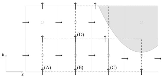
Figure 1.
Main grid (solid gray lines) with immersed solid (gray area) showing displaced velocity components and four u-cell types (dashed black lines): (A) and (B) interior cells, (C) and (D) cut cells.
The strength of convection F, and diffusion conductance D are given by Equations (8) and (9)
where are the advecting velocities, are the distances to east, west, north and south neighbors.
Figure 2 presents a more general case involving a cut cell where the areas and distances are truncated. Special procedures are needed in this case to evaluate the convection and diffusion contributions. Refer to Kirkpatrick et al. [17] for more details on the methodology.
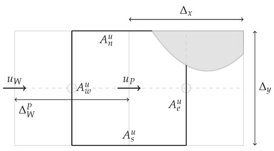
Figure 2.
Cut u-cell showing areas and lengths used in the discretization.
3.2. Advected Velocity Component Treatment for Interior Cells
This section develops three different methods that will be utilized to determine the advected velocity component on the faces: upwind, QUICK and WAHYD (TVD). The above methods consider all neighbors as interior cells but allow unequal distances with the center P.
The general form corresponds to an upwinded deferred-correction scheme, which for the east face results in
Resulting source terms have the form etc. Note that for the upwind scheme one has .
As in [17], the QUICK scheme can be derived considering flow direction and that the second partial derivatives are constant , . When put in the form of Equation (10), resulting source terms for the east face are
where as before, symbols indicate distances between 2 and 1.
For the WAHYD scheme of [26], the source terms are computed in the following manner
3.3. Interpolation Details for the Convective Term
Following Kirkpatrick et al. [17], the velocity nodes on the main grid faces which are cut by the solid boundary are displaced to the center of the face segment that remains in the fluid, as shown in Figure 1. For an interior u-cell such as case (A), see Figure 1, there are no displacements for its velocity components. However, for interior u-cell (B) and cut u-cells (C) and (D), velocity components are displaced to the center of their cut faces and special interpolation procedures are needed. Consider the cut u-cell Case (D), which is set apart in Figure 3. Here, is displaced since the vertex lies within the solid body. In order to estimate the advecting velocity component , a simple linear interpolation can be used
where and are the distances among velocities in the n face shown in Figure 3. Note that this procedure can also be used in case of interior u-cells (A) and (B), and will subsequently be referred as A-scheme.
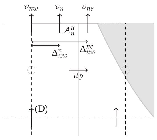
Figure 3.
Case (D) cut u-cell interpolation for at cut face , , on fluid.
Depending on the interface position, or can end up being located inside the solid, see Figure 4. In this case, the A-scheme would over/under-estimate the velocity. Instead, an interpolation alternative that uses a point on the interface (also referred as an auxiliary point), can be considered. This interpolation scheme will be labeled B-scheme and it is presented in Equation (19)
with the y velocity component of the boundary.
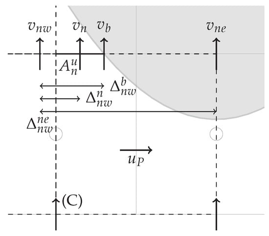
Figure 4.
Case (C) cut u-cell interpolation for at cut face , on fluid, on solid and on interface.
The vicinity of the interface may result in a situation as depicted in Figure 5 in which the (east) neighbor node is displaced due to the presence of the solid body. In this case, Kirkpatrick calculates the advecting velocity using Equation (20). The correction is due to the fact that the linear estimate is not necessarily located at the center of the east face, see the dashed line joining and in Figure 5.
where is the x velocity component of the boundary, h and are the normal distances to the solid boundary of and respectively. In case ends up located inside the solid, an auxiliary point on the solid surface is used for the interpolation. If the east face is cut, the auxiliary point is located in the north or south face of the cell, depending on the solid boundary orientation, as shown in Figure 6, and is calculated using Equation (20). If the east face is uncut, the auxiliary point is located moving horizontally from , as shown in Figure 7.
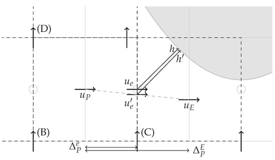
Figure 5.
Interpolation for near solid boundary. is the resulting interpolation between and , which is corrected to the face center with the distances to the solid boundary h and .
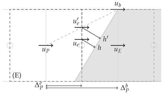
Figure 6.
Limit case of interpolation for near solid boundary in which is cut, is within the solid and .
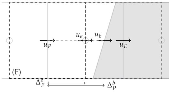
Figure 7.
Interpolation for near solid boundary in which is uncut, is within the solid and .
3.4. Interpolation Details for the Diffusive Term
Near a solid interface, as shown in Figure 8, the vector that goes from to is not perpendicular to the east face, Kirkpatrick suggest the diffusive term to be calculated using Equation (21). In case is located inside the solid, auxiliary points are used for calculation, as explained previously for the determination of
with vector defined from to , is the y component of the unit normal vector , and is the normal vector from surface that intersects in the e face.
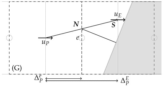
Figure 8.
Computation for diffusive contribution requires vector defined from to and normal vector from surface which intersects with in the e face.
3.5. Interpolation Details for the Source Term
Source terms that take into account the effect of pressure and shear due to the presence of the solid must be added to the momentum equation [27]. With reference to Figure 9 and for the cut-cell scheme, this gives Equation (22)
where l is the (wet) area of the solid body within the cell, is the x component of the unit normal vector .
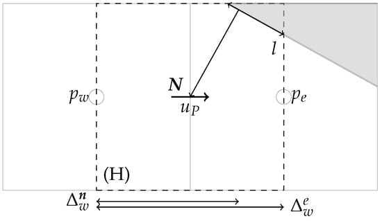
Figure 9.
Computation for force requires normal vector from surface which intersects with and area l of solid body.
3.6. Classification of Small Cells
With reference to Figure 2 consider the following relations
where is an adjustable parameter to obtain different levels of refinement in the (cut cell) geometrical representation. For a given grid and we obtain the most refined geometric representation, while will give a more staircase shape similar to the Voxel method.
3.7. Numerical Solution
The SIMPLE algorithm of Patankar [25] was used to treat the pressure-velocity coupling. Fully implicit discretized equations were solved using a parallel implementation of the ADI/TDMA algorithm [28] in an in-house C/OMP code. All simulations were conducted until the normalized residues were below for the momentum and continuity equations. For comparisons between results, the definition of computational efficiency given in [29] was used
where K is a constant arbitrarily fixed that depends on the machine used, e is some measurement of the numerical prediction error, is the computation time.
4. Results
4.1. Flow between Concentric Cylindrical Walls
Figure 10 presents the schematic of a laminar flow driven by a momentum source between concentric cylindrical walls. Similar to Sato et al. [3], we compared the numerical results with the analytical solutions for the velocity field. Additionally, we give the pressure field analytic solution in the present work.
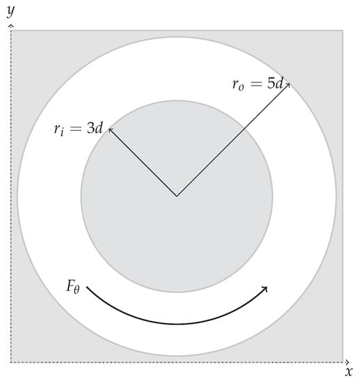
Figure 10.
Geometry considered for the case of flow between concentric cylindrical walls.
Considering the r and components of Equation (2), and adding a volumetric force as a source term for the equation results in
which upon integration using the no-slip requirement at the walls, provides the analytical solutions for the velocity and stress
Solving for the pressure requires the determination of a constant at a position where the pressure is known. Choosing for , and defining , the analytical dimensionless pressure profile is
Consider the error norm for the velocity as
where is the numerical value of the theta component dimensionless velocity at i-cell obtained with the interpolation scheme, N is the number of cells within the region of interest .
Numerical results were obtained using the three methods described in Section 3.2, and grids , , , , , for physical parameters equivalent to a . With these kappa values chosen, and as stated in Section 3.6, small -cells will be designated as those which areas of their cut flow faces and/or the corresponding areas of the main cells cut flow faces are under 2, 20 and 40% of their respective uncut areas .
Table 1 presents the number and percentage of slave cells generated as function of and the grid size. These numbers correspond to either the u or v cut cells since, given the geometry studied, their numbers turned out the same. As expected, the proportion of slave cells increases with the value of , being more cut cells classified as slave cells with this rise in tolerance. Moreover, the percentage of slave cells increases when the grid is coarser due to the resulting lower geometry resolution for the immersed solid body representation. Figure 11 presents the distribution of fluid, slave and solid cells near the solid boundaries. Notice that for the distribution of slave cells mimics an enlargement of the solid body’s dimensions. The amount of slave cells generated with reduces the apparent dimension of the solid body but produces less smoothness on the body surface. Lastly, with the solid body is represented more accurately with a smoother surface since less slave cells are produced.

Table 1.
Number of u or v slave cells generated and their percentage (in parenthesis) over total u or v cut cells for the flow between concentric cylindrical walls case as function of and the grid size.
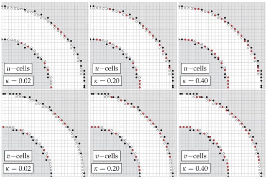
Figure 11.
Fluid (white), solid (black) and slave (red) cells distribution around the immersed solids for the flow between cylindrical walls case with the grid.
Figure 12, Figure 13 and Figure 14 present the errors plotted against the grid spacing where it can be seen that, for the upwind method, a less than first order tendency was obtained, whereas the QUICK and WAHYD schemes, supra linear behavior was achieved. These degradations in the order of accuracy for cut-cell methodologies had been observed in the literature [17], and explained as the possible result of irregularities of the mesh near the solid boundaries affecting the local error. In the three methods studied, a big difference in magnitude in the errors was observed when using compared to , where no major differences were detected.
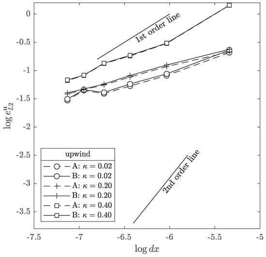
Figure 12.
Velocity error norm as function of the interpolation schemes and parameter for the flow between concentric cylinders case using the upwind method.
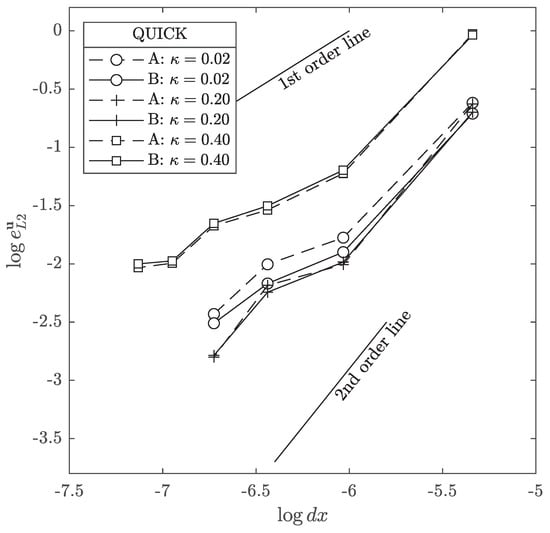
Figure 13.
Velocity error norm as function of the interpolation schemes and parameter for the flow between concentric cylinders case using the QUICK method.
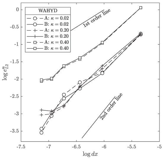
Figure 14.
Velocity error norm as function of the interpolation schemes and parameter for the flow between concentric cylinders case using the WAHYD method.
Figure 15 and Figure 16 illustrate the dependency observed for the computational efficiency with the values. In the present case, the solid bodies are represented by circumferences and the results indicate that, regardless of the grid used, the lower values of favor the computational efficiency. The QUICK and WAHYD schemes gave higher efficiency values than the upwind scheme. Although small, generally the B interpolation scheme produced a more efficient algorithm than the A alternative for each method at the smallest values of .
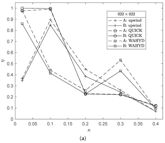
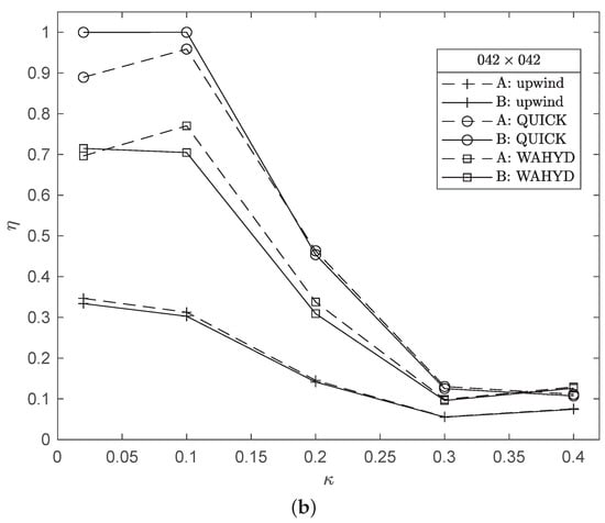
Figure 15.
Computational efficiency as function of for the flow between concentric cylinders case and grids: (a) 22 × 22, (b) 42 × 42.
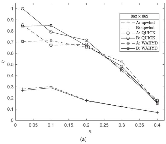
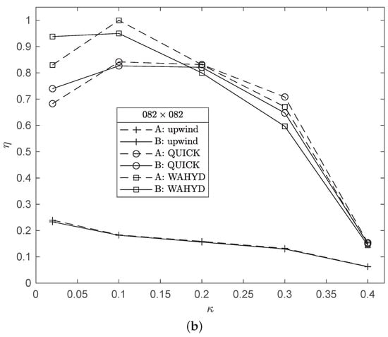
Figure 16.
Computational efficiency as function of for the flow between concentric cylinders case and grids: (a) 62 × 62, (b) 82 × 82.
Figure 17 presents the dimensionless velocity and pressure profiles for the cases with the lowest numerical error obtained. A good agreement of the higher-order methods in the dimensionless velocity profile can be observed, whereas the upwind scheme underpredicts the velocity peak due to its diffusive nature. Following the same argument, the sigmoidal-like dimensionless pressure profile is better represented by the QUICK and WAHYD numerical solutions than the upwind scheme, at least in a shape-preserving manner for the relatively coarse grids used.
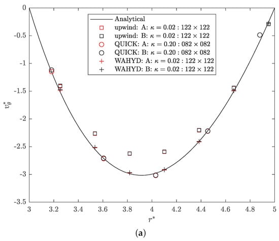
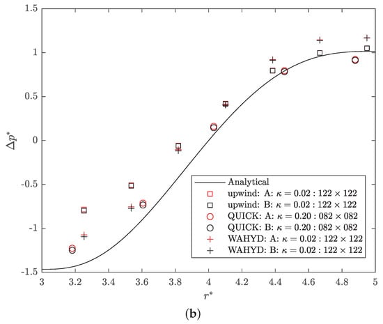
Figure 17.
Analytical and best numerical solutions found for the flow between concentric cylindrical walls case, . (a) dimensionless velocity; (b) dimensionless pressure.
4.2. Flow on a Inclined Channel
Figure 18 depicts the flow on an inclined channel situation. For the coordinate system, making a momentum balance gives
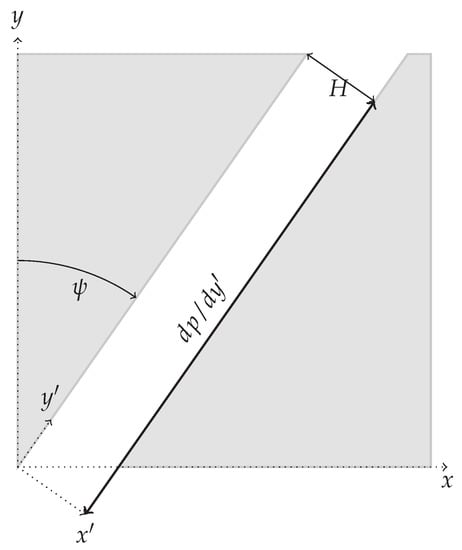
Figure 18.
Geometry considered for the case of flow on a inclined channel.
Considering , one has as analytical solution for the velocity component
A velocity error difference between the A and B interpolation schemes can be defined as
Simulations were performed for , angles , grid sizes and . Parameters were adjusted to give .
Table 2 and Table 3 display cut-cell details obtained as function of and Figure 19 and Figure 20 present their distribution for the 22 × 22 grid and and three values of . Similar tendencies to those of Table 1 are observed, but in the present situation there is some asymmetry in the origination of cut cells and slave cells which increases with , since no symmetry plane can be found parallel to x or y coordinates. Figure 21 presents the errors for all cases considered. Similar error profiles are found for both grids, with the coarser one having its magnitudes larger for the angles studied. For values of , and for both grids, the B interpolation scheme performed better than A (i.e., ). For other values of the geometrical refinement parameter , positive values of the error difference can be seen. Nevertheless, the magnitudes of the negative errors are bigger than the positive ones, and these bigger negative values are found in the region of more geometrical refinement. These trends are more pronounced in the cases with greater slope. Figure 22 presents the dimensionless velocity profiles, where it can be seen that the three methods employed, i.e., upwind, QUICK and WAHYD, produced similar solutions.
Table 2.
Number of u slave cells generated and their percentage (in parenthesis) over total u cut cells for the inclined channel flow case as function of , and grid size.
Table 3.
Number of v slave cells generated and their percentage (in parenthesis) over total v cut cells for the inclined channel flow case as function of , and grid size.
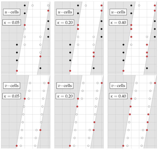
Figure 19.
Fluid (white), solid (black) and slave (red) cells distribution around the immersed solids for the inclined channel flow case with the grid and °.
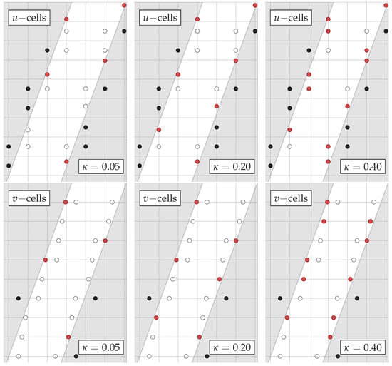
Figure 20.
Fluid (white), solid (black) and slave (red) cells distribution around the immersed solids for the inclined channel flow case with the grid and °.
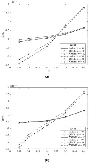
Figure 21.
Velocity error norm difference as function of parameter and , for the flow on inclined channel case. (a) grid; (b) .
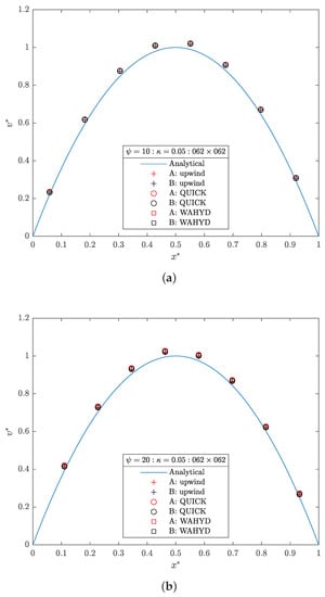
Figure 22.
Dimensionless velocity profile for the flow on inclined channel case. (a) ; (b) .
Figure 23 and Figure 24 present the computational efficiency obtained for the cases studied as a function of . Different from the tendency shown in the flow between concentric cylinders case, the higher efficiency values are obtained with the mid-to-high values of . This difference may be due to the type of curve that represents the immersed solid body, which in the present case are two straight lines, whereas in the former case they were circumferences. Nevertheless, the maximum-to-minimum computational efficiency ratio is higher for the flow between concentric cylinders case than in the present one, suggesting a greater effect of on the computational efficiency when the streamlines are curved.
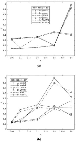
Figure 23.
Computational efficiency as function of for the flow on a skewed-channel case using grid 22 × 22 and : (a) 10°, (b) 20°.
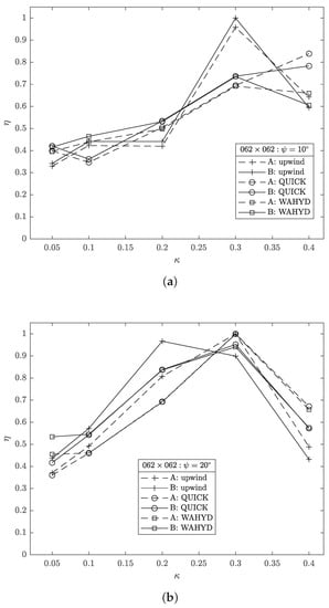
Figure 24.
Computational efficiency as function of for the flow on a skewed-channel case using grid 62 × 62 and : (a) 10°, (b) 20°.
4.3. Flow around a Circular Cylinder
Two-dimensional flow around a single cylinder was simulated for Reynolds numbers 7, 10 and 20. Domain size was 40D in the transverse direction and 60D in the streamwise direction. The cylinder center was located at the coordinates (20D, 20D), see Figure 25. Boundary conditions of the complete domain were established as uniform velocity profile at the left boundary, outlet at right boundary. Bottom and top boundaries were set as symmetry. No-slip at the cylinder surface. Results of the contributions to the drag coefficient and the pressure coefficient are considered as in [30]
and the dimensionless pressure
with normal vector at cylinder surface, viscous stress tensor, D cylinder diameter, r cylinder radius, upstream velocity and pressure.
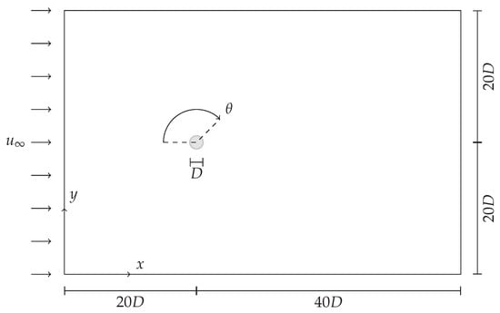
Figure 25.
Geometry considered for the case of flow around a cylinder.
Three values of and five nonuniform structured grids were used with a finer section of size centered around the cylinder. Table 4 presents the cases considered and the percentage of slave cells generated. Figure 26 presents part of their distribution on the vicinity of the solid body. To evaluate surface derived quantities, interpolation for missing surface points was performed using piecewise cubic Hermite interpolating polynomials. Considering the treatment of slave cells, the higher value of value (0.40) gives the impression of a cylinder with an effective diameter greater than the original body. The intermediate value of (0.20) produces a less smooth surface but with better approximation of the true solid dimension. Finally, the lower value of better approximates the solid body shape both on smoothness and its real dimension.
Table 4.
Grid sizes used for the flow around a cylinder case.
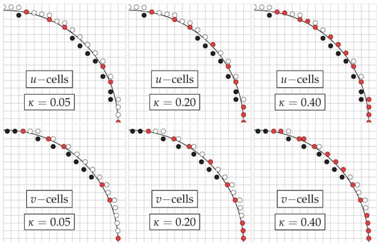
Figure 26.
Fluid (white), solid (black) and slave (red) cells distribution around the immersed solid for the flow around a cylinder case with the E grid.
Numerical computation of magnitudes was performed for each case of Table 4 and their deviation with respect to reference values taken from [30] was computed as
where denotes the references, absolute error of numerical estimation of , combined error of numerical predictions.
Figure 27, Figure 28, Figure 29 and Figure 30 present the absolute error of as function of the grid size and the extremes values of used for Re = 20 and both interpolation approaches. It can be seen that smaller errors are obtained with and the B interpolation scheme, although influence of the interpolation is more modest on the profiles. Results for g20 and g30 grids are almost the same, implying that convergence of the numerical procedure is achieved with these grid sizes. Similar profiles were obtained for Re = 7, 10 but their figures are not presented to avoid extending the manuscript. Figure 31 presents the combined errors of the four previously studied quantities as function of the Reynolds number for each interpolation scheme and method used. As expected, on account of its greater numerical diffusion, the upwind method presented larger combined error compared to the higher-order alternatives. Regardless of the method and the Reynolds number, the difference observed in the combined error is about 1% in favor of the B interpolation scheme.
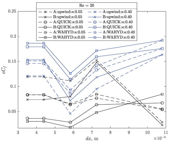
Figure 27.
Drag coefficient error as function of grid size for the flow around a cylinder case with Re = 20.
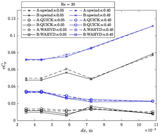
Figure 28.
Pressure coefficient error as function of grid size for the flow around a cylinder case with Re = 20.
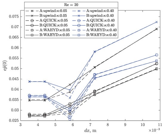
Figure 29.
Dimensionless pressure error at as function of grid size for the flow around a cylinder case with Re = 20.
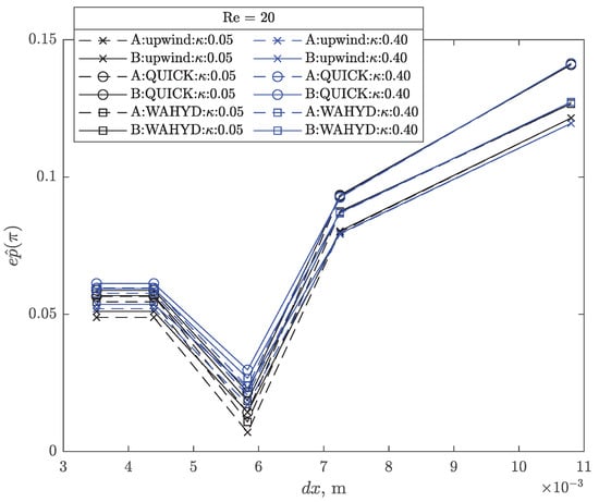
Figure 30.
Dimensionless pressure error at as function of grid size for the flow around a cylinder case with Re = 20.
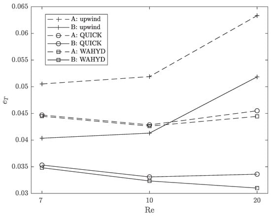
Figure 31.
Total error as function of Re for the flow around a cylinder case using and the E grid.
Figure 32, Figure 33 and Figure 34 show the computational efficiency as function of for each Reynolds number used. Similar to the flow between concentric cylindrical walls case, which used curves instead of lines to represent the solid body, the bigger values of are shifted towards the smaller values of .
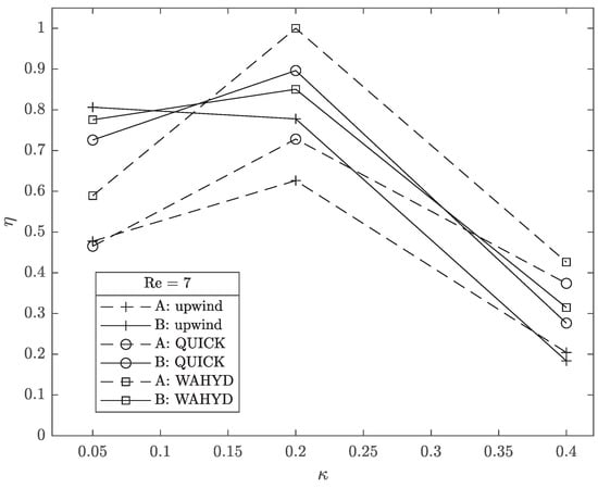
Figure 32.
Computational efficiency as function of for the flow around a cylinder case with Re = 7 using the E grid.
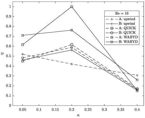
Figure 33.
Computational efficiency as function of for the flow around a cylinder case with Re = 10 using the E grid.
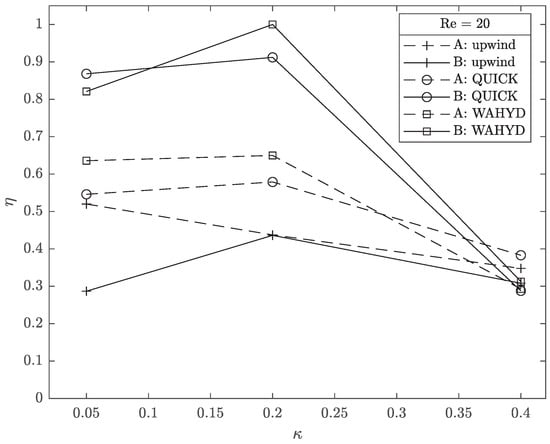
Figure 34.
Computational efficiency as function of for the flow around a cylinder case with Re = 20 using the E grid.
5. Conclusions
The number of slave cells generated increases with the value resulting in an apparent enlargement of the solid body dimensions accompanied by an erosion of the smoothness of its interfacial surface. This interpretation is bounded to the treatment given to the generated slave cells but, nonetheless, a higher number of slave cells around the body representation are likely to introduce more errors to the numerical solution.
It was empirically found that smaller values of favor the computational efficiency of the numerical solution of problems that include an immersed solid represented by circumferences. Conversely, larger values of are paired with larger computational efficiency for problems characterized by solids represented by straight lines.
The B interpolation scheme produces less error and higher computational efficiencies than the A scheme, regardless of the quadric shape used to represent the solid body, when it is paired with low values of . The effect is generally small in the error comparison but higher in the computational efficiency. The improvement of the B scheme over the A scheme is of more significance when evaluating magnitudes which depend on gradient estimations at surfaces.
The effects described for choices of and interpolation scheme are valid for all the advected velocity component treatments tested, namely, upwind, QUICK and WAHYD (TVD).
Author Contributions
Conceptualization, L.H.-V., F.A. and L.L.; methodology, L.H.-V. and F.A.; software, L.H.-V., F.A. and L.L.; validation, L.H.-V., F.A. and P.D.-G.; formal analysis, L.H.-V. and F.A.; investigation, L.H.-V. and F.A.; resources, L.H.-V. and L.L.; data curation, L.H.-V., F.A. and P.D.-G.; writing—original draft preparation, L.H.-V. and F.A.; visualization, L.H.-V. and P.D.-G.; supervision, L.H.-V.; funding acquisition, L.H.-V. and P.D.-G. All authors have read and agreed to the published version of the manuscript.
Funding
The APC was funded by DICYT-USACH Universidad de Santiago de Chile.
Institutional Review Board Statement
Not applicable.
Informed Consent Statement
Not applicable.
Data Availability Statement
Not applicable.
Acknowledgments
The authors thank the support of PFCHA CONICYT NACIONAL/2017 22170013. Powered@NLHPC: This research was partially supported by the supercomputing infrastructure of the NLHPC (ECM-02) and by the high-performance computing system of PIDi-UTEM (SCC-PIDi-UTEM CONICYT-FONDEQUIP-EQM180180).
Conflicts of Interest
The authors declare no conflict of interest. The funders had no role in the design of the study; in the collection, analyses, or interpretation of data; in the writing of the manuscript, or in the decision to publish the results.
Abbreviations
The following abbreviations are used in this manuscript:
| QUICK | Quadratic Upstream Interpolation for Convective Kinematics |
| WAHYD | Water Resources Management and Modeling of Hydrosystems |
| TVD | Total Variation Diminished |
| ADI | Alternating Direction Implicit |
| TDMA | Tri-Diagonal Matrix Algorithm |
References
- Mittal, R.; Iaccarino, G. Immerse Boundary Methods. Annu. Rev. Fluid Mech. 2005, 37, 239–261. [Google Scholar] [CrossRef] [Green Version]
- Ingram, D.; Causon, D.; Mingham, C. Developments in Cartesian cut cell methods. Math. Comput. Simul. 2003, 61, 561–572. [Google Scholar] [CrossRef]
- Sato, N.; Takeuchi, S.; Kajishima, T.; Inagaki, M.; Horinouchi, N. A consistent direct discretization scheme on Cartesian grids for convective and conjugate heat transfer. J. Comput. Phys. 2016, 321, 76–104. [Google Scholar] [CrossRef]
- Berger, M.; Aftosmis, M. Progress Towards a Cartesian Cut-Cell Method for Viscous Compressible Flow. In Proceedings of the 50th AIAA Aerospace Sciences Meeting including the New Horizons Forum and Aerospace Exposition, Nashville, TN, USA, 9–12 January 2012. [Google Scholar] [CrossRef] [Green Version]
- Peskin, C.S. Flow patterns around heart valves: A numerical method. J. Comput. Phys. 1972, 10, 252–271. [Google Scholar] [CrossRef]
- Fadlun, E.; Verzicco, R.; Orlandi, P.; Mohd-Yusof, J. Combined Immersed-Boundary Finite-Difference Methods for Three-Dimensional Complex Flow Simulations. J. Comput. Phys. 2000, 161, 35–60. [Google Scholar] [CrossRef]
- Kim, J.; Kim, D.; Choi, H. An Immersed-Boundary Finite-Volume Method for Simulations of Flow in Complex Geometries. J. Comput. Phys. 2001, 171, 132–150. [Google Scholar] [CrossRef]
- Kajishima, T.; Takiguchi, S. Interaction between particle clusters and particle-induced turbulence. Int. J. Heat Fluid Flow 2002, 23, 639–646. [Google Scholar] [CrossRef]
- Mittal, R.; Dong, H.; Bozkurttas, M.; Najjar, F.; Vargas, A.; von Loebbecke, A. A versatile sharp interface immersed boundary method for incompressible flows with complex boundaries. J. Comput. Phys. 2008, 227, 4825–4852. [Google Scholar] [CrossRef] [Green Version]
- Liu, C.; Hu, C. An immersed boundary solver for inviscid compressible flows. Int. J. Numer. Methods Fluids 2017, 85, 619–640. [Google Scholar] [CrossRef]
- Berger, M. A Note on the Stability of Cut Cells and Cell Merging. Appl. Numer. Math. 2015, 96, 180–186. [Google Scholar] [CrossRef] [Green Version]
- Dechristé, G.; Mieussens, L. A Cartesian cut cell method for rarefied flow simulations around moving obstacles. J. Comput. Phys. 2016, 314, 465–488. [Google Scholar] [CrossRef] [Green Version]
- Chung, M.H. An adaptive Cartesian cut-cell method for conjugate heat transfer on arbitrarily moving fluid-solid interfaces. Comput. Fluids 2019, 178, 56–72. [Google Scholar] [CrossRef]
- Ye, T.; Mittal, R.; Udaykumar, H.; Shyy, W. An accurate Cartesian grid method for viscous incompressible flows with complex immersed boundaries. J. Comput. Phys. 1999, 156, 209–240. [Google Scholar] [CrossRef] [Green Version]
- Chung, M.H. Cartesian cut cell approach for simulating incompressible flows with rigid bodies of arbitrary shape. Comput. Fluids 2006, 35, 607–623. [Google Scholar] [CrossRef]
- Colella, P.; Graves, D.T.; Keen, B.J.; Modiano, D. A Cartesian grid embedded boundary method for hyperbolic conservation laws. J. Comput. Phys. 2006, 211, 347–366. [Google Scholar] [CrossRef] [Green Version]
- Kirkpatrick, M.; Armfield, S.; Kent, J. A representation of curved boundaries for the solution of the Navier-Stokes equations on a staggered three-dimensional Cartesian grid. J. Comput. Phys. 2003, 184, 1–36. [Google Scholar] [CrossRef]
- Hartmann, D.; Meinke, M.; Schröder, W. An adaptive multilevel multigrid formulation for Cartesian hierarchical grid methods. Comput. Fluids 2008, 37, 1103–1125. [Google Scholar] [CrossRef]
- Hartmann, D.; Meinke, M.; Schröder, W. A Cartesian Cut-Cell Solver for Compressible Flows. In Computational Science and High Performance Computing IV; Krause, E., Shokin, Y., Resch, M., Kröner, D., Shokina, N., Eds.; Russian-German Advanced Research Workshop on Computational Science and High Performance Computing (4th:2009:Freiburg, Germany); Springer: Berlin/Heidelberg, Germany, 2011; pp. 363–376. [Google Scholar]
- Grove, A.S.; Shair, F.H.; Petersen, E.E. An experimental investigation of the steady separated flow past a circular cylinder. J. Fluid Mech. 1964, 19, 60–80. [Google Scholar] [CrossRef]
- Dietiker, J.F.; Guenther, C.; Syamlal, M. A Cartesian cut cell method for gas/solids flows. In Proceedings of the AIChE Annual Meeting, Nashville, TN, USA, 8–13 November 2009. [Google Scholar]
- Li, T.; Dietiker, J.F.; Shahnam, M. MFIX simulation of NETL/PSRI challenge problem of circulating fluidized bed. Chem. Eng. Sci. 2012, 84, 746–760. [Google Scholar] [CrossRef]
- Dietiker, J.F.; Li, T.; Garg, R.; Shahnam, M. Cartesian grid simulations of gas-solids flow systems with complex geometry. Powder Technol. 2013, 235, 696–705. [Google Scholar] [CrossRef]
- Xie, Z.; Stoesser, T. A three-dimensional Cartesian cut-cell/volume-of-fluid method for two-phase flows with moving bodies. J. Comput. Phys. 2020, 416, 109536. [Google Scholar] [CrossRef]
- Patankar, S. Numerical Heat Transfer and Fluid Flow, 1st ed.; Hemisphere Publishing Corporation: Philadelphia, PA, USA, 1980. [Google Scholar]
- Hou, J.; Simons, F.; Hinkelmann, R. Improved total variation diminishing schemes for advection simulation on arbitrary grids. Int. J. Numer. Methods Fluids 2011, 70, 359–382. [Google Scholar] [CrossRef]
- Ferziger, J.; Peric, M. Computational Methods For Fluid Dynamics, 3rd ed.; Springer: Berlin/Heidelberg, Germany, 2002. [Google Scholar]
- Henríquez-Vargas, L.; Villaroel, E.; Gutierrez, J.; Donoso-García, P. Implementation of a parallel ADI algorithm on a finite volume GPU-based elementary porous media flow computation. J. Braz. Soc. Mech. Sci. Eng. 2017, 39, 3965–3979. [Google Scholar] [CrossRef]
- Fletcher, C. Computational Techniques For Fluid Dynamics 1, 2nd ed.; Springer: Berlin/Heidelberg, Germany, 1990. [Google Scholar]
- Dennis, S.C.R.; Chang, G.Z. Numerical solutions for steady flow past a circular cylinder at Reynolds numbers up to 100. J. Fluid Mech. 1970, 42, 471–489. [Google Scholar] [CrossRef]
Publisher’s Note: MDPI stays neutral with regard to jurisdictional claims in published maps and institutional affiliations. |
© 2022 by the authors. Licensee MDPI, Basel, Switzerland. This article is an open access article distributed under the terms and conditions of the Creative Commons Attribution (CC BY) license (https://creativecommons.org/licenses/by/4.0/).