Article

Rigid-Flexible Coupling Dynamics Modeling of Spatial Crank-Slider Mechanism Based on Absolute Node Coordinate Formulation

1
School of Mechanical Engineering and Automation, Northeastern University, Shenyang 110819, China
2
AECC Shenyang Engine Research Institute, Shenyang 110015, China
*
Author to whom correspondence should be addressed.
Mathematics 2022, 10(6), 881; https://doi.org/10.3390/math10060881
Submission received: 8 February 2022 / Revised: 27 February 2022 / Accepted: 4 March 2022 / Published: 10 March 2022

Abstract

:
In order to study the influence of compliance parts on spatial multibody systems, a rigid-flexible coupling dynamic equation of a spatial crank-slider mechanism is established based on the finite element method. Specifically, absolute node coordinate formulation (ANCF) is used to formulate a three-dimensional, two-node flexible cable element. The rigid-flexible coupling dynamic equation of the mechanism is derived by the Lagrange multiplier method and solved by the generalized α method and Newton–Raphson iteration method combined. Comparison of the kinematics and dynamics response between rigid-flexible coupling system and pure rigid system implies that the flexible part causes a certain degree of nonlinearity and reduces the reaction forces of joints. The elastic modulus of the flexible part is also important to the dynamics of the rigid-flexible multibody system. With smaller elastic modulus, the motion accuracy and reaction forces become lower.

1. Introduction

Multibody systems are composed of several rigid or flexible objects interconnected by joints, which are applied in various fields, such as aviation, robots and vehicle systems. With the development of industry, more and more mechanical systems demand spatial movement [1,2], which requires further analysis of spatial multibody systems.
The fundamental problem of multibody system dynamics is modeling and computation. Since the 1960s, many scholars have studied multibody systems. Wittburg [3] published research work on multibody system dynamics, which laid the foundation for the Lagrange method for multibody system dynamics. Nikravesh [4] focused on computer-aided analysis of multibody systems and discussed the modeling and calculation of multibody systems in detail. Haug and Habana [5,6] put forward the Cartesian method of modeling multi-rigid-body systems. Computational multibody system dynamics research can be divided into rigid multibody systems, flexible multibody systems and rigid-flexible coupling multibody systems according to the mechanical characteristics of objects existing in the system. The term multi-rigid body system refers to a system in which all objects are rigid and elastic deformation can be ignored. The term flexible multibody system refers to the large-scale elastic deformation of objects during the movement of the system. A rigid-flexible coupling system is a rigid multibody system with some flexible parts [7,8,9,10].
Rigid-flexible coupling multibody dynamics is becoming more and more important especially for spacecraft structures, and the deformation of flexible bodies can cause complex nonlinear mechanical behaviors to the multibody system [11,12,13]. Traditionally, machines are assumed to be rigid bodies for multibody dynamics analysis. However, with the growing demand of higher precision and resolution it is necessary to consider the influence of component deformation. In fact, each component of a mechanical system has deformation under loading. In order to simplify the calculation and modeling, some components with tiny deformations of the mechanical system can be regarded as rigid bodies. The rigid-flexible coupling system takes into account the deformation of flexible bodies, and also considers calculation efficiency and simplicity [13,14,15,16,17,18,19].
The crank-slider system, as a basic mechanism, is widely used in various fields. For those mechanisms running at high speed and large scale, the influence of the flexibility cannot be ignored, otherwise it would reduce the precision of the system, and make dynamics characteristics seriously different from real system [20,21]. Different modeling methods to study the kinematics and dynamics of the crank-slider system have been proposed. Liu [22] established the slider-crank mechanism model and studied the kinematics and dynamics of offset slider-crank mechanism. Li et al. [23] studied the dynamics of the crank-connecting rod system with clearance and flexible rod, and discussed the influence of flexible connecting rod on the mechanism. Qian et al. [24] analyzed the kinematics and dynamics of the crank-slider mechanism based on Simulink in MATLAB. Ma et al. [25,26,27] simulated the dynamics of the planetary gear train based on the virtual prototype technology. Wu et al. [28,29] conducted simulation research on multibody dynamics mechanisms of a crank connecting rod mechanism based on Adams, and provided a simulation idea of multibody dynamics. The above-mentioned research is basically for rigid planar crank-slider mechanisms, while research on spatial crank-slider mechanisms with flexible component is rare. In this paper, the spatial crank-slider mechanism is formulated, and the flexible rod is established based on the absolute node coordinate formulation, and the rigid-flexible coupling dynamic equation of spatial crank-slider mechanism is derived by the Lagrange multiplier equation to analyze the influence of flexible rod on spatial crank-slider mechanism.

2. Cable Model Based on ANCF Method

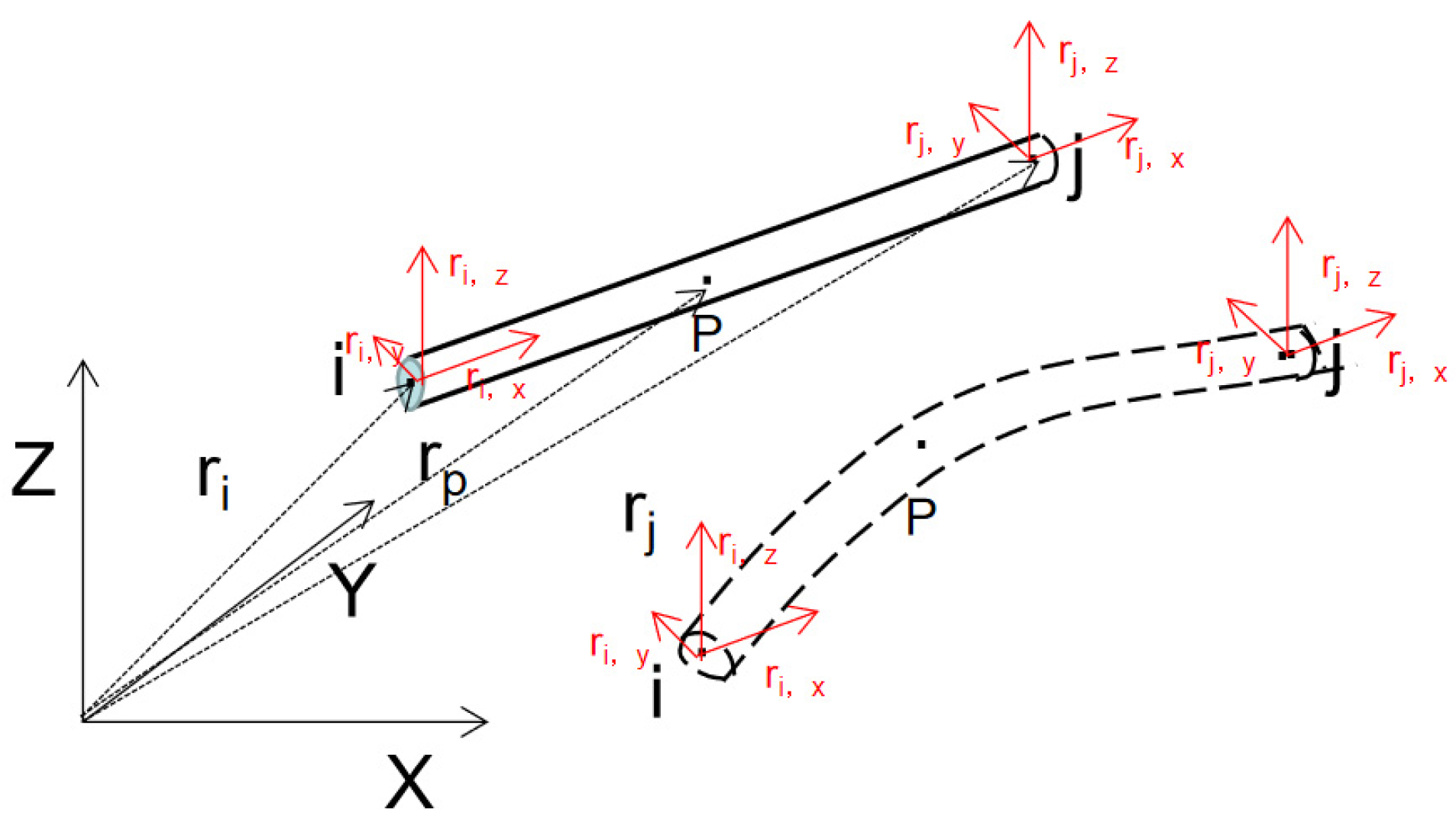
2.1. ANCF Cable Element Model

In this paper, the cable element based on ANCF [30,31] is used for modeling flexible component, as shown in Figure 1, r x     r y   r z   represents the body coordinate system, the end points of the element are i and j respectively, P is any point in the element r i r j r p are the position vectors in the absolute coordinate system.
The generalized coordinate vector r p of any point p in the flexible cable element can be expressed as
r p ( x ) = S ( x ) [ r i r ix r j r jx ]
r = [ S 1 I 2 S 2 I 2 S 3 I 2 SI 2 ] q e
S 1 = 1 2 x 2 + 3 x 3 S 2 = l ( x 2 x 2 + 3 x 3 ) S 3 = 3 x 2 2 x 3 S 4 = l ( x 2 + x 3 )
where, x is the local coordinate in the axial direction (the first node i x   = 0); l is the reference length of finite element rod before deformation; S is the shape function of the rod element; I 2 is a second-order identity matrix; q e is a generalized coordinate vector with eight node coordinates, which can be expressed as
q e = [ e 1 e 2 e 3 e 4 e 5 e 6 e 7 e 8 ] T = [ r i 1 r i 2 r i 1 x r i 2 x r j 1 r j 2 r j 1 x r j 2 x ] T
where, the vector [ r k 1 r k 2 ] T ( k = i , j ) is the coordinate of the absolute position of the cable element node in the absolute coordinate system; r k x ( k = i , j ) represents the absolute position slope of the cable element in the absolute coordinate system and the tangential direction of the axis. As a spatial ANCF flexible cable, the position coordinates of any point on the element can be expressed as
r p = [ X Y Z ] = S ( x , y , z ) q e ( t ) q e = [ r i T r i x T r i y T r i z T r j T r j x T r j y T r j z T ] T S = [ s 1 I 3 s 2 I 3 s 3 I 3 s 4 I 3 s 5 I 3 s 6 I 3 s 7 I 3 s 8 I 3 ]
where,
s 1 = 1 3 ζ 2 + 2 ζ 3 ,   s 2 = l ( ζ 2 ζ 2 + ζ 3 ) s 3 = l ( ψ ζ ψ ) ,   s 4 = l ( ξ ζ ξ ) s 5 = 3 ζ 2 2 ζ 3 ,   s 6 = l ( ζ 2 + ζ 3 ) s 7 = l ζ ψ ,   s 8 = l ζ ξ ζ = x / l ,   ψ = y / l ,   ξ = z / l
It can be seen that there are 24 generalized coordinates of the three-dimensional ANCF cable element, which are respectively composed of the position coordinates at the nodes and the coordinate vectors describing directions.

2.2. Element Mass Matrix

The unit mass matrix of the cable can be obtained from kinetic energy, which requires the velocity of any point in the element, and the velocity of any point P in the element can be expressed as
r x = S q e ˙  
The kinetic energy of the cable element can be expressed as
T = 1 2 V   ρ r x T r x dV = 1 2 q ˙ e T M q ˙ e
The mass matrix of the cable element can be obtained as follows
M = ρ V   S T SdV .
where v is the volume of the element; ρ is the density of material; M is the element mass matrix. r x =   r x   = r . and r xx = 2 r x 2 .

2.3. Generalized Elastic Force of Element

u is the displacement vector of any point along the axis and the deformation gradient J is
J = u v
where r is the position vector in the element body coordinate system.
U = 1 2 0 l ( EA ε x 2 + EI κ 2 ) dx
where U is the strain energy of the cable element.
The virtual work of elasticity can be defined as
δ W e = L   [ EA ε x δ ε x + EI κ δ κ ] dx
where
ε x = 1 2 ( J 2 1 ) = 1 2 ( r x T r x 1 )
κ = | r x × r xx | | r x | 3
where E is the elastic modulus; A is the cross-sectional area; I is the inertia tensor; ε x is the axial Green-Lagrangian strain;   κ is the bending curvature.
Assuming that
ξ = x / l ,   0 < = ξ < = 1 f = | r x × r xx | , g = | r x | 3
δ κ = κ q e δ q e = 1 g 2 ( g f q e f g q e ) δ q e
Then the generalized internal force Q e can be expressed as
Q e = L   EI 1 g 2 ( g f q e f g q e ) d ξ + L   3 EA ( r x T r x ) 1 2 ( r x T r x q e ) d ξ
The mass matrices of all ANCF elements are constant, but the internal elastic force is extremely nonlinear in coordinates.

2.4. Generalized External Force of Element

When external force F acts on a certain point of ANCF cable element, the virtual work done by the force F at that point can be calculated by the principle of virtual work. When the force F g is gravity, the virtual work can be calculated as
δ W g = F g δ r = g V   ρ dV · S δ q e = gm · S δ q e = Q g T δ q e
Q g = ρ V   [ 0 0 g ] SdV = S T ( mg )
where, Q g is the external force of gravity and g is the acceleration of gravity.
The dynamics formula is derived as follows
M q ¨ e = Q g + Q e

3. Rigid-Flexible Coupling Dynamic Model

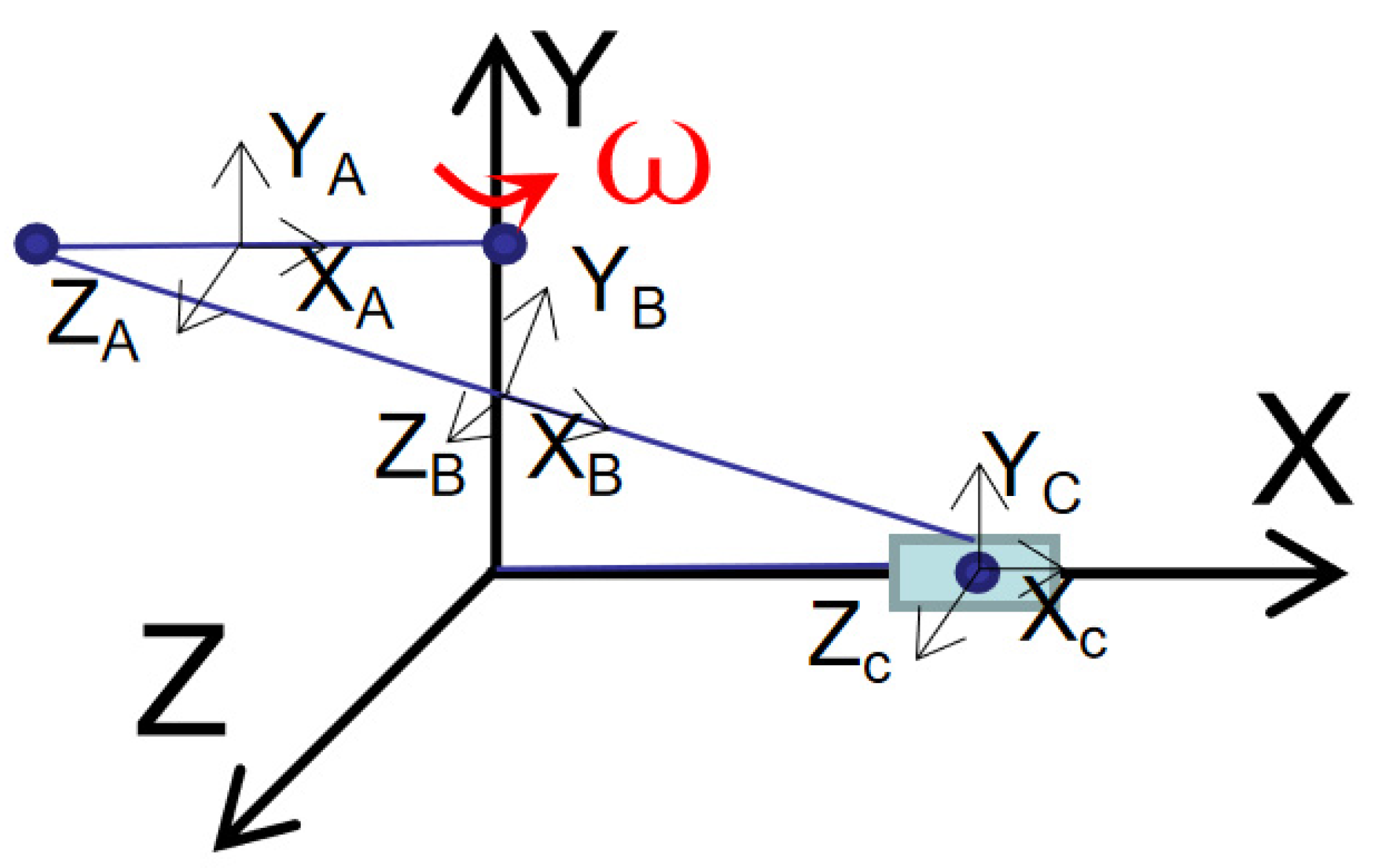
3.1. Mechanism Analysis

As shown in Figure 2, the spatial crank-slider mechanism is composed of crank A, connecting rod B and slider C, in which connecting rod B is assumed to be flexible, and the degree of freedom m = 1 can be obtained according to the Kutzbach criterion. The rigid bodies in the crank-slider system are established by the natural coordinate method, while the flexible connecting rod B is established by the ANCF.
In order to formulate constraint equations of spatial multibody system, it is necessary to set up an inertial coordinate system for the adjacent components connected by the same kinematic joint to describe the spatial orientation and position of the components. As shown in Figure 2, an inertial coordinate system is established at the centroid point of the rod to express the subsequent kinematic position. The crank is set as the driving part, with angular velocity ω = π / 10 rad / s clockwise.
The crank and ground are connected by rotating joint and spherical joints are formulated at both ends of the connecting rod with the crank and slider.
The constraint equation of rotating joint is established as follows.
Φ s ( P i , P j ) = 0 Φ P 1 ( h i ,   h j ) = 0
where Φ P 1 is the equation ensuring hi and hj parallel to each other, Φ s is the constraint equation of spherical joint, joint point on component i and j are P i and P j respectively. f, g and h are the unit vectors of local coordinate system.
Φ P 1 ( h i ,   h j ) = [ Φ d 1 ( f i , h j ) Φ d 1 ( g i , h j ) ] = [ f i T · h j g i T · h j ] = 0
Φ d 1 means the inner product of two vectors is zero, where the rotation around XY direction is constrained.
The constraint equation of the spatial moving pair is
Φ p 1 = ( h i ,   h j ) = 0 Φ p 2 = ( h i ,   d ij ) = 0 Φ d 1 = ( f i ,   f j ) = 0
where d ij = r i P r j P , r i P and r j P are the absolute coordinate vectors of P point on i and j component respectively. The constraint equations keep the slider move along the x-axis
For rigid bodies, unknown Cartesian coordinate q and constraint equations can be established as follows
q i = [ r i p i ]
Φ ( q ,   t ) [ Φ Κ ( q ) Φ D ( q ,   t ) Φ p ( q ) ] = 0
where, Φ Κ ( q ) is the kinematic constraint.   Φ D ( q , t ) is the driving constraint.   Φ p ( q ) is Euler parameter constraint. r i is the position vector of inertia coordinate of each component.   p i is the Euler parameter of the inertia coordinate of each component.
The Jacobian of the constraint equation is
Φ q = [ Φ q K Φ q D Φ q P ]
Φ q Δ q ( j ) = Φ ( q ( j ) ,   t ) q ( j + 1 ) = q ( j ) + Δ q ( j )
Given an estimated initial value q ( 0 ) , q can be calculated by Newton-Raphson iteration Formula (26). The constraint equation between rigid components and flexible component is formulated as below, where r 0 and r n are the node position vectors of the flexible component, while r B 1 and r B 2 are node position vectors of the rigid component.
Φ 1 = [ r ( 0 ) r B 1 r ( n ) r B 2 ] = 0

3.2. Rigid-Flexible Coupling Dynamic Equation

The rigid-flexible coupling dynamic equation of space crank-slider is constructed. The mass matrix of flexible components formulated by ANCF is constant, so there is no centrifugal force or Coriolis force. Mass matrix of rigid components M r and flexible components M f are formulated as below,
M r = diag ( m i ,   m i ,   m i ,   I ix ,   I iy ,   I iz )
M f = ρ V   S T SdV
The spatial rigid-flexible coupling dynamic equation is obtained as follows, which can be solved by generalized α method and Euler implicit method combined.
{ M Σ q ¨ + Φ q T λ = Q + Q e Φ ( q ,   t ) = 0
M Σ = [ M r 0 0 M f ] ,   q = [ q r q f ]

4. Numerical Simulation and Analysis

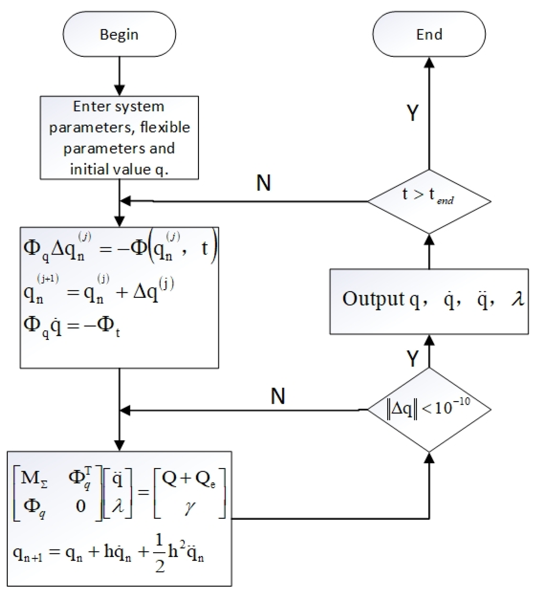
4.1. Simulation Process and Parameters

The fully rigid spatial slider-crank mechanism and rigid-flexible coupling spatial slider-crank mechanism are analyzed respectively. The related parameters are shown in Table 1.
The flow chart for solving the dynamic equation of the spatial rigid-flexible coupling crank-slider mechanism is shown in Figure 3. The Newton–Raphson iterate method is used, and the specific steps are as follows: ① Input system parameters and initial value q ( 0 ) at time t = 0. System parameters mainly include mass, moment of inertia and dimension of each component, elastic modulus and the element nodes of flexible component. ② Through the Newton–Raphson iteration formula, the speed and approximate position at this moment are calculated. If the numerical value obtained by the Newton–Raphson method can’t reach the convergence result, the initial value can be iterated by qn+1 in Figure 3 to select a suitable initial value. Smaller step size and suitable iteration value can improve the convergence of the algorithm. ③ Start calculation of the rigid-flexible coupling dynamic equation. The acceleration of components and the reaction force at the constraint joints are estimated, if the error requirement is met, go to next time step and iteration again until the end time.

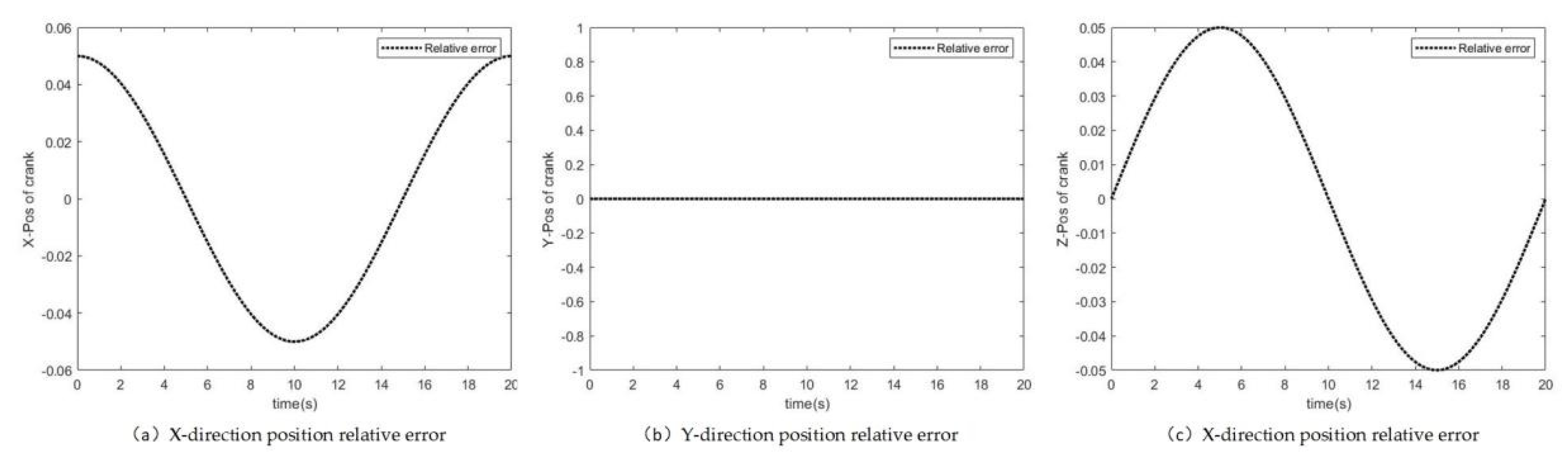
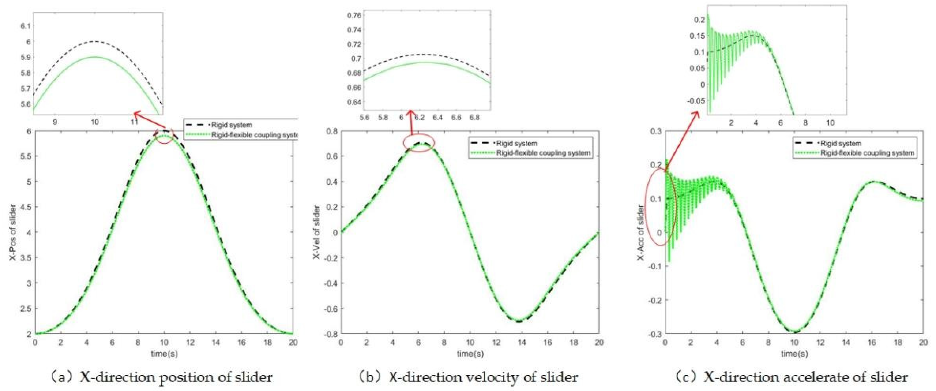
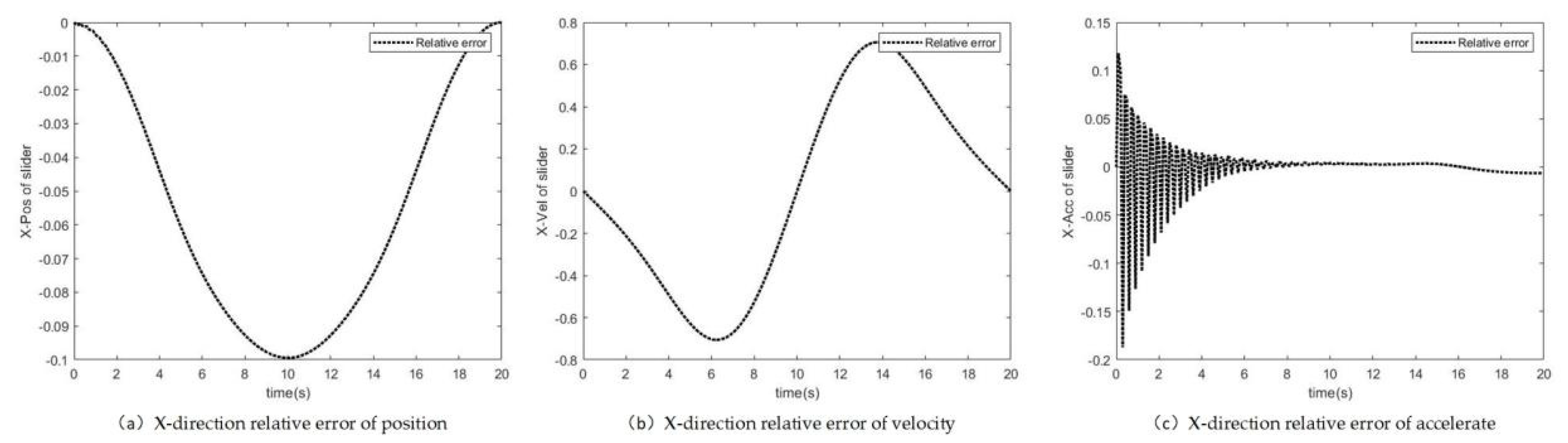
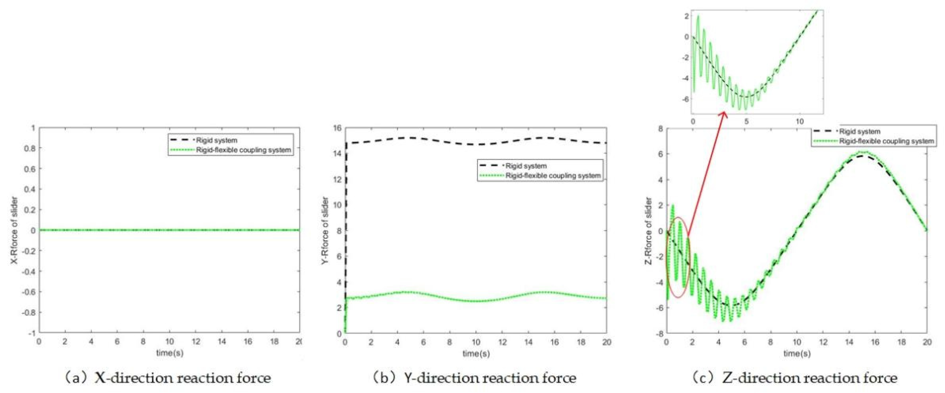
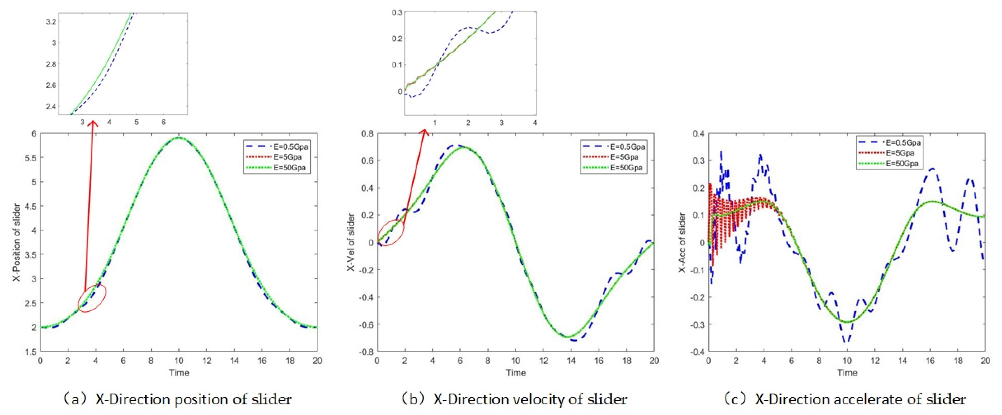
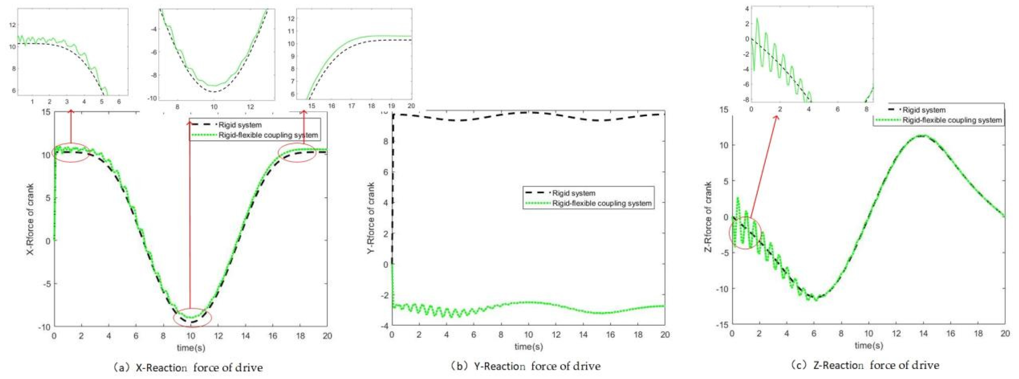
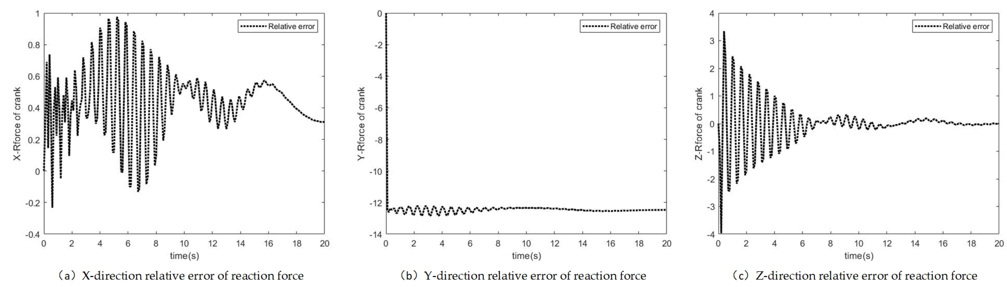
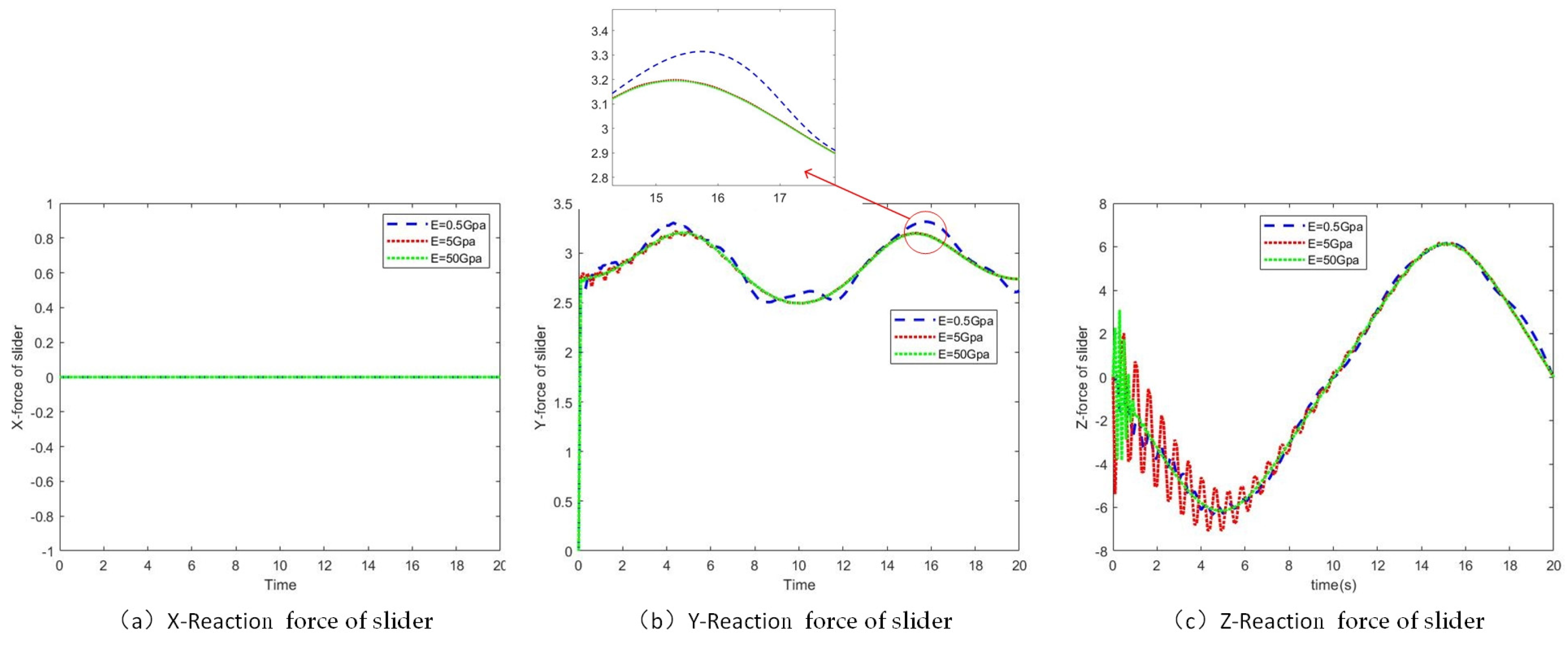
4.2. Analysis of Simulation Results

Kinematics and dynamics of spatial rigid and spatial rigid-flexible coupling slider-crank mechanisms are carried out. The time step is 0.1 s and the total simulation time is 20 s. The crank rotates around the Z axis with angular velocity of π / 10 rad / sin clockwise, and external force −10 N is applied on the slider along the X direction. The comparison of slider kinematics and dynamics between the rigid and rigid-flexible coupling systems is shown in Figure 4, Figure 5, Figure 6, Figure 7, Figure 8, Figure 9 and Figure 10. It can be seen that generally the difference between the rigid-flexible coupling system and the pure rigid system is obvious. The results along Y and Z directions are not considered since the slider moves along the X direction in absolute coordinates.
Figure 4 and Figure 5 shows the displacement of the joint between the crank and connecting rod and the relative displacement difference. It can be seen that the displacement along three coordinate axes basically coincide. The displacement of the rigid-flexible coupling system is slightly lower than that of the rigid system because of elastic force. The maximum displacement difference in the X and Z direction is 0.05 m. It can be concluded that the influence of flexible parts on the displacement of joint is not significant.
Figure 6 shows the comparison of displacement, velocity and acceleration of the slider between the two systems and the relative difference is shown in Figure 7.
It can be seen that the displacement and velocity basically coincide with each other, the largest difference of displacement is about 0.1 m located at the peak, and the maximum difference of velocity is 0.05 m/s and also located around peak. At the beginning, the acceleration of the rigid-flexible coupling system fluctuates, which is due to the instantaneous rigid impact caused by initial momentum and force. The impact generates the elastic force of the flexible body and finally leads to the vibration of the system. The vibration gradually vanished due to the damping and energy loses inside the flexible component. The acceleration tends to coincide with the increase of time.
Reaction forces of the crank drive and the relative difference are shown in Figure 8 and Figure 9. The maximum difference in the X direction is about 1 N accompanied by fluctuation. The relative difference of the amplitude gradually decreases. The difference of the driving reaction force in the Y direction of the two system is about 12 N, which is due to the stretching action of the flexible part. The fluctuation of reaction forces at the initial period comes from the elastic forces of the flexible part resisting the driving impact. The maximum difference of the reaction force in the Z direction is about 4 N.
Figure 10 shows the reaction force at the rotation joint between the slider and the connecting rod. The reaction force in the X direction of the joint is zero. The difference in the reaction force in the Y direction is about 12 N, which is similar to the reaction force of drive. The reaction force in the Z direction vibrates initially with a maximum amplitude of 5 N, which is caused by the impact from driving, and the two curves tend to become consistent gradually with the increase of time.
Figure 11 shows the kinematics response of the slider of the rigid-flexible coupled system with different elastic modulus. The displacements are basically consistent with a slight difference of 0.05 m around 4 s. Therefore, the elastic modulus has little influence on the displacement. While a smaller elastic modulus causes stronger fluctuation of velocity with a maximum difference of 0.1 m/s, acceleration presents a larger amplitude of vibration with lower frequency when the elastic modulus is small and the maximum amplitude of vibration is observed at the initial time, which is 0.2 m/s2, and then decreases with time.
Figure 12 shows the reaction force at the rotation joint of the slider with different elastic modulus. The reaction force in the X direction is basically zero, while the reaction force in the Y direction changes obviously, and the maximum difference is about 0.2 N. The reaction forces with different elastic modulus in the Z direction are also very obvious. With larger elastic modulus, the reaction force undergoes stronger vibration in the initial period but shorter duration. The possible reason for this phenomenon lies in the greater elastic modulus that implies stronger rigidity of the flexible part against deformation, and therefore a smaller vibration amplitude and recovery with high frequency.
Higher elastic modulus of flexible components may contribute to larger reaction forces but a smaller fluctuation range of acceleration.

5. Conclusions

Based on the absolute node coordinate formulation, this paper formulates a three-dimensional ANCF flexible connecting rod with nine cable elements, establishes the rigid-flexible coupling dynamic equation, and numerically solves the rigid-flexible coupling equation. The kinematics and dynamics of the rigid space crank-slider system and rigid-flexible coupling space crank-slider system are compared, and the influence of the flexible component on motion accuracy and reaction forces is obtained. It can be inferred that the existence of an internal elastic force causes the rigid-flexible coupling system to fluctuate greatly. Finally, the kinematic and dynamic responses of the rigid-flexible coupled system with different elastic modulus are analyzed. The results show that a smaller elastic modulus has a greater influence on motion accuracy and reaction forces.
Spatial deficient ANCF beam formulation coupled with spatial rigid body dynamics proposed in this paper represents and advance for rigid-flexible multibody dynamics, which are mostly focused on planar mechanisms. The analysis of the influence of different elastic coefficients on system dynamics has significance for flexible component design.

Author Contributions

Conceptualization, X.W.; data curation, H.W.; formal analysis, H.W.; funding acquisition, C.X.; methodology, X.W.; project administration, Z.L.; resources, X.W. and C.X.; software, X.W.; supervision, Z.L. and Q.H.; visualization, H.W. and J.Z.; writing–original draft, H.W.; writing–review & editing, X.W. All authors have read and agreed to the published version of the manuscript.

Funding

This work was supported by the National Natural Science Foundation of China (52005088) and the Natural Science Foundation of Liaoning Province (2020-MS-076) and National Science and Technology Major Project (J2019-IV-0002-0069).

Institutional Review Board Statement

Not applicable.

Informed Consent Statement

Not applicable.

Data Availability Statement

No reported data.

Conflicts of Interest

The authors declare no conflict of interest.

References

  1. Dias, J.; Pereira, M.S. Sensitivity Analysis of Rigid-Flexible Multibody Systems. Multibody Syst. Dyn. 1997, 1, 303–322. [Google Scholar] [CrossRef]
  2. Youwu, L. Application of multi-body dynamics in mechanical engineering. China Mech. Eng. 2000, 11, 6. [Google Scholar]
  3. Wittenburg, J.; Likins, P. Dynamics of Systems of Rigid Bodies. J. Appl. Mech. 1977, 45, 458. [Google Scholar] [CrossRef]
  4. Nikravesh, P.E.; Chung, I.S. Application of Euler Parameters to the Dynamic Analysis of Three-Dimensional Constrained Mechanical Systems. J. Mech. Des. 1982, 104, 785–791. [Google Scholar] [CrossRef]
  5. Haug, E.J.; Wu, S.C.; Yang, S.M. Dynamics of mechanical systems with Coulomb friction, stiction, impact and constraint addition-deletion—III Spatial systems. Mech. Mach. Theory 1986, 21, 401–406. [Google Scholar] [CrossRef]
  6. Shabana, A.A. Definition of the Slopes and the Finite Element Absolute Nodal Coordinate Formulation. Multi-Body Syst. Dyn. 1997, 1, 339–348. [Google Scholar] [CrossRef]
  7. Garcia-Vallejo, D.; Mayo, J.; Escalona, J.L.; Domínguez, J. Three-dimensional formulation of rigid-flexible multibody systems with flexible beam elements. Multibody Syst. Dyn. 2008, 20, 1–28. [Google Scholar] [CrossRef]
  8. Zhang, C. Mechanical Dynamics, 2nd ed.; Higher Education Press: Beijing, China, 2008. [Google Scholar]
  9. Jiazhen, H.; Chaolan, Y. Research progress of rigid-flexible coupling system dynamics. J. Dyn. Control. 2004, 2, 6. [Google Scholar]
  10. Jiazhen, H.; Zhuyong, L. Modeling method of rigid-flexible coupling dynamics. J. Shanghai Jiaotong Univ. 2008, 42, 5. [Google Scholar]
  11. Jiazhen, H.; Lizhong, J. Rigid-flexible coupling dynamics of flexible multi-body system. Mech. Prog. 2000, 30, 6. [Google Scholar]
  12. Likins, P.W. Finite element appendage equations for hybrid coordinate dynamic analysis. Int. J. Solids Struct. 1972, 8, 709–731. [Google Scholar] [CrossRef]
  13. Bakr, E.M.; Shabana, A.A. Geometrically nonlinear analysis of multi-body systems. Comput. Struct. 1986, 23, 739–751. [Google Scholar] [CrossRef]
  14. Lin, B.; Xie, C. Dynamics of Flexible multi-body Systems. Acta Mech. Sin. 1989, 4, 469–478. [Google Scholar]
  15. Yigi, S.A. The Effect of Flexibility on the Impact Response of a Two-Link Rigid-Flexible Manipulator. J. Sound Vib. 1994, 177, 349–361. [Google Scholar] [CrossRef]
  16. Choura, S.; Yigit, A.S. Control of a Two-Link Rigid–Flexible Manipulator with a Moving Payload Mass. J. Sound Vib. 2001, 243, 883–897. [Google Scholar] [CrossRef]
  17. Williams, D.; Fredrickson, G.H. Cylindrical Micelles in Rigid-Flexible Diblock Copolymers. MRS Online Proc. Libr. 1991, 248, 3561–3568. [Google Scholar] [CrossRef]
  18. Duan, Y.C.; Zhang, D.G. Rigid-Flexible Coupling Dynamics of a Flexible Robot with Impact. Adv. Mater. Res. 2011, 199, 243–250. [Google Scholar] [CrossRef]
  19. Zhao, F.; Liu, J.; Hong, J. Nonlinear dynamic analysis on rigid-flexible coupling system of an elastic beam. Theor. Appl. Mech. Lett. 2012, 2, 023001. [Google Scholar] [CrossRef] [Green Version]
  20. Bai, Z.F.; Zhao, Y.; Tian, H. Study on collision dynamics of flexible multibody system. J. Vib. Shock. 2009, 28, 75–78+195–196. [Google Scholar]
  21. Wang, J.M.; Hong, J.Z. Experimental Study on Flexible Multibody Dynamics. J. Astronaut. 1999, 2, 108–112. [Google Scholar]
  22. Mo, L. Kinematics and dynamics analysis of crank-slider mechanism based on MATLAB. Automot. Pract. Technol. 2019, 23, 135–137. [Google Scholar] [CrossRef]
  23. Li, T.T.; Zhang, Z.S.; Cui, G.H.; Guan, L.Z. Dynamic analysis of crank-connecting rod mechanism with coupling hinge clearance and flexibility. Mech. Transm. 2021, 45, 116–122. [Google Scholar] [CrossRef]
  24. Qian, Y.; Cao, Y.; Liu, Y.W.; Zhou, H. Forward Kinematics Simulation Analysis of Slider-Crank Mechanism. Adv. Mater. Res. 2011, 308–310, 1855–1859. [Google Scholar] [CrossRef]
  25. Ma, X.G.; Lu, Y.; You, X.M. Multi-body dynamics simulation analysis of planetary gear train based on multi-body dynamics technology. China Mech. Eng. 2009, 20, 1956–1959+1964. [Google Scholar]
  26. Liu, Y.H.; Miu, B.Q. Theoretical basis and functional analysis of multi-body dynamics simulation software ADAMS. Electron. Packag. 2005, 5, 5. [Google Scholar]
  27. Shi, Z.X.; Fung, E.; Lie, Y.C. Dynamic modelling of a rigid-flexible manipulator for constrained motion task control. Appl. Math. Model. 1999, 23, 509–525. [Google Scholar] [CrossRef]
  28. Wu, M.Q.; Mei, H.F.; Zhang, Z.Q. Multi-body dynamics simulation of linkage mechanism based on ADAMS. J. Eng. Des. 2005, 12, 4. [Google Scholar]
  29. Fan, B.L.; Yang, G.H.; Zhu, X.Y. Research and practice teaching of crank-connecting rod mechanism based on multi-body dynamics simulation. Met. World 2021, 1, 71–75. [Google Scholar]
  30. Sugiyama, H.; Escalona, J.L.; Shabana, A.A. Formulation of Three-Dimensional Joint Constraints Using the Absolute Nodal Coordinates. Nonlinear Dyn. 2003, 31, 167–195. [Google Scholar] [CrossRef]
  31. Shabana, A.A. Computational Continuum Mechanics; Cambridge University Press: Cambridge, UK, 2012. [Google Scholar]
Figure 1. ANCF cable element model.
Mathematics 10 00881 g001
Figure 2. Schematic diagram of spatial crank-slider model.
Mathematics 10 00881 g002
Figure 3. Flow chart of calculation.
Mathematics 10 00881 g003
Figure 4. Displacement of crank-connecting rod joint.
Mathematics 10 00881 g004
Figure 5. Relative displacement difference of connecting rod joint.
Mathematics 10 00881 g005
Figure 6. Comparison of kinematic parameters of slider in X direction.
Mathematics 10 00881 g006
Figure 7. Relative kinematic parameters difference of slider in X direction.
Mathematics 10 00881 g007
Figure 8. Reaction force of drive.
Mathematics 10 00881 g008
Figure 9. Relative reaction force difference of drive.
Mathematics 10 00881 g009
Figure 10. Reaction force of rotation joint of slider.
Mathematics 10 00881 g010
Figure 11. Kinematics response of slider with different elastic modulus.
Mathematics 10 00881 g011
Figure 12. Reaction force of slider rotating joint with different elastic modulus.
Mathematics 10 00881 g012
Table 1. Mechanism parameter.
ComponentCrank AConnecting Rod BSlider C
I x / k g · m 2 0.0050.0050.05
I y / k g · m 2 0.10.10.05
I z / k g · m 2 0.10.10.05
Mass/kg10.51
Length/m2 17 0.4
Section Diameter/m/0.03/
Young’s Modulus/Pa/5 × 109/
Number of Elements/9/
Publisher’s Note: MDPI stays neutral with regard to jurisdictional claims in published maps and institutional affiliations.

