Abstract
The classical backward bending of the labor supply curve has been extended to the case of the inverted S-shaped labor supply curve during the last three decades. According to this extension, at very low net wage levels near the subsistence income level, the positive shape of the supply curve of labor may also be curved backward and become negatively sloped. A decrease in the low wage rate requires an increase in the labor supply, to maintain a minimum income level for survival. The S-shaped curve leads to a double-peaked Laffer curve, which also includes the possibility of three tax rates, each of which enables the collection of the same tax revenue. This may occur in contrast to the traditional single-peaked Laffer curve, which has two tax rates with the same revenues.
Keywords:
multi-peaked Laffer curve; backward-bending supply curve; inverted labor supply; net wage rate MSC:
80M50
1. Introduction
The classical approach to the shape of the Laffer curve is based on the idea of the backward-bending labor supply curve. Following the work of Hanoch [1], this approach indicates that a backward bending of the labor supply curve necessarily leads to the classical bell-shaped Laffer curve with one peak. However, during the last couple of decades, other economists have introduced a new shape of the labor supply curve, with an inverted S-shaped labor supply. This new shape of labor supply curve leads to a new shape of the Laffer curve, with more than one peak point.
The purpose of the following model is to challenge the conventional classical approach advocated by Arthur Laffer and many other experts. Their approach is that the relationship between tax revenues and tax rates imposed on employees necessarily creates a bell-shaped curve that contains one peak point. The model developed below leads to a new shape of the Laffer curve, with at least two peak points. The uniqueness of the model is that using a specific combination of utility functions generates an inverted S-shaped labor supply, resulting in a Laffer curve that has at least two peak points.
2. A Review of Approaches to the Labor Supply
The following discussion describes the differences between two approaches to labor supply. The first considers a backward-bending labor supply, while the new second approach is based upon an inverted S-shaped labor supply, resulting in new shapes of the Laffer curve.
2.1. The Labor Supply Curve
For several decades economists who have dealt with the relationship between net wage rate and the quantity of daily working hours supplied, have assumed backward-bending curves (Varian [2], Nicholson and Snyder [3], Sharif [4,5,6], Dessing [7], Barzel and McDonald [8], Lin [9], Riley and Szivas [10], and Eisenhauer [11]). Assuming that the utility function of any wage earner depends positively both on income from work and on leisure hours during the twenty-four-hour day, several implications were derived regarding labor supply. Based on the assumption that leisure is a normal good, and according to many social science researchers even a luxury item with income elasticity that is greater than one, most economists conclude that there is an hourly reservation net wage rate, below which the worker does not supply labor services. Furthermore, an increase in the net wage rate above the reservation net wage rate will increase the willingness of the worker to supply more working hours and maintain fewer leisure hours, due to the dominant substitution effect. However, an additional increase in the net wage rate may lead to approaching a certain point of the wage rate at which the income effect is dominant. In such a scenario, an increase in the net wage rate leads simultaneously to an increase in both the net income used for consumption, as well as in the hours required for leisure.
Spiegel and Templeman [12] and Tavor et al., [13] introduced special utility functions of the worker that, indeed, lead to a certain reservation net wage rate at which the labor supplied is zero, a certain net wage rate at which the labor supply is at maximum, and a range of net wage rates at which the influence on the quantity of labor supplied is negative (this is referred to as the range of backward bending of the labor supply curve).
2.2. The Inverted S-Shaped Labor Supply Curve
An important extension to the classical backward bending of the labor supply was introduced a few decades ago by Sharif [4,5,6], Dessing [7], and others, such as Hanoch [1], Barzel and McDonald [8], Lin [9], Riley and Szivas [10], and Eisenhauer [11], with the theory of the ‘inverted S-shaped labor supply curve’. Hanoch [1] discusses and proposes an extension of the backward-bending labor supply curve, due to conflicting income and substitution effects. Suppose leisure is an inferior good or a normal good with a low-income effect. In that case, the dominant substitution effect leads to an increasing labor supply, due to a wage increase up to a certain turning point, at which the income effect on leisure is positive, high, and dominant. Thus, labor supply decreases as a result of the wage increase at high wage rates. According to this extension, at very low net wage levels, near the subsistence income level, the positive slope of the supply curve of labor may also be curved backward and become negatively sloped. Several theoretical and empirical works consider this issue.
The shape of the labor supply at a very low net wage rate demonstrates a hyperbolic curve, where reduction in the net wage rate requires an increase in the labor supply, i.e., the labor supply curve is negatively sloped. In recent years, this possible shape of the labor supply curve has been introduced in different industries in which the basic net wages are very low. Among the recent papers dealing with subsistence survival are theoretical and empirical works concerning the existence of subsistence income.
Several empirical works and examples of increased labor of poor workers with a decrease in wages show that in different industries, such as tourism and agriculture, these workers need to survive and guarantee subsistence income. This is very common in very poor countries and among very poor individuals (usually children and unskilled women and men in faltering industries). Several citations relevant to this discussion are provided below. Hussain et al. [14] discuss the socio-economic determinants that influence children’s work. Parents compel them to leave school and join the labor force to guarantee subsistence income. Thus, lower wage rates require a greater supply of child labor. A very similar phenomenon is discussed by Luckstead et al. [15], who found that in the cocoa industry, the low price of the cocoa final good enables employers to hire workers such as children at a very low wage. This low wage that is paid to the children guarantees them a subsistence income.
The phenomenon of the downward sloping labor supply curve is applicable to explanations of behavior in tourism, as presented by Riley and Szivas [10]. Based on a study in Tarapith Temple Town, West Bengal, Masud [16] claims that tourism provides the prospect for developing a poor region. Local people are attracted to jobs and income from tourism, for their subsistence. According to Nguyen et al. [17], tourism in Ha Long, Vietnam is a potential catalyst for transforming subsistence marketplaces, and the quality of life (QOL) for people who live in them. An additional example is provided by Mathew [18], who claims that at higher levels of income, secondary workers may re-enter the market when they have more employment opportunities due to better education, by transferring some of their household chores to the market. This eases their double burden of balancing work and family. Accordingly, the labor supply curve assumes an S-shape [19,20,21]. The thesis of ‘added worker effect’ also establishes that secondary workers enter the labor force in response to a fall in family income [22,23,24]. Adhering to the theoretical base of the joint labor supply model, this paper analyzes labor market outcomes in the Kasargod district, using unit-level data from employment and unemployment surveys by the National Sample Survey Office (NSSO).
3. The Laffer Curve
The shape of the classical Laffer curve is based on the phenomenon of the backward-bending labor supply curve. This approach indicates that a backward bending of the labor supply curve necessarily leads to the classical bell-shaped Laffer curve with one peak. During the last couple of decades, economists have introduced a new shape of the labor supply curve, with an inverted S-shaped labor supply. Eisenhauer ([11], p. 195), Figure 5 illustrates an inverted S-shaped labor supply curve. He shows the circumstances that can form the basis of labor supply with inflection points. The inflection points of the labor supply configuration are necessary to guarantee the Laffer curve with inflection points, i.e., more than one peak point. Gärtner et al. [25] used a similar inverted S-shaped labor supply curve of children on p. 240, Figure 5. This is due to the requirement that children work for the sake of subsistence income that they supply to their family. It is important to emphasize again that the inverted S-shaped labor supply curve generates a Laffer curve with multiple inflection points. Similar findings, with regards to the inverted S-shaped labor supply curve, are also presented by Nakamura and Yu Murayama [21] p. 673 Figure 5.
When the net wage rate is too low, an increase in the labor supply is required to maintain a minimum income level for survival. These subsistence requirements lead to the situation in which, at some very low ranges of the net wage rates, the supply curve is hyperbolic. A certain percentage decrease in the net wage rate leads to the same percentage increase in the labor supply. This additional range of the curve leads to what is called the inverted S-shaped labor supply curve, which may end at an extremely low net wage rate. At such a rate, so many hours are necessary to maintain the subsistence requirement that the worker stops working. Instead of working as an employee, he may prefer to be self-employed, thereby working and producing for self-production and his own consumption. He, thus, could avoid earning as an employee, paying income taxes, etc. In another publication, Dessing [7] repeats the argument regarding the inverted S-shaped labor supply curve, while deriving an interesting implication. Under certain conditions in which the minimum wage rate is very low, an increase may stabilize the labor market at a higher wage combined with lower values of unemployment.
The use of some utility functions described above (e.g., [12,21]), which lead to the specific inverted S-shaped labor supply curve, and more specifically that at low net wage rate lead to the phenomenon of a downward labor supply, might be considered at this stage, only as a solid intellectual exercise discussed by theoretical economists. However, in recent years empirical economists have revealed that this can be considered as a realistic phenomenon in some industries in which the net wage is significantly low. Riley and Szivas [10] suggest the following basic proposition: The labor supply curve can slope downwards, indicating that people expand supply as the rate of pay declines, just for the sake of survival. The authors argue that this is characteristic of the tourism industry. They follow the theoretical contribution of Sharif [4,5,6], who uses the term ‘distress selling of labor’. This term indicates that the very poor have no realistic leisure options. Included among them are working mothers, who may work more hours when their rate of pay declines. They need to earn the subsistence income required for the sake of their survival and that of their children. A few years later, Song et al. [26] repeated the same discussion of the downward labor supply in the tourism industry.
A recent extension of the special Laffer curve was developed by Fève et al. [27]. This unique Laffer curve is referred to by the authors as the horizontally S-shaped Laffer curve. It leads to the possibility of obtaining the same tax revenues at three different tax rates imposed on employee salaries. Fève et al. ([27], p. 884) explain that ‘…there can be up to three tax rates associated with the same level of fiscal revenues’. This result guarantees a Laffer curve with at least one peak point at a determined tax rate, followed by a trough point with a higher tax rate and then another peak point with a third tax rate.
During recent years, and especially in empirical studies concerning the Laffer issue, the curve has been used as by Boqiang and Zhijie [28], who explored the relationship between tax rates and government revenue. Based on a Chinese data set, they found that the top of China’s Laffer curve is about 40%. Boqiang and Zhijie [28] examined the relationship between the direct tax rate on labor income and tax revenues, as well as real economic activity. Their analysis was based on the presumption of a single-peaked Laffer curve using a data set of the Chinese market. A similar work in Spain, which examined the relationship between the marginal tax rates and the tax revenue, was also based on a single-peaked Laffer curve. In that work, Sanz-Sanz [29] used data sets from Spain and performed calculations for the individual taxpayer, as well as the aggregate population for the aggregate Laffer curve. This was characterized as a single hump-shaped Laffer curve. The paper of Fève et al. [27] is an exception, since they used a neoclassical growth model with an incomplete and heterogeneous market. The purpose of their work was to prove that in special cases, using the inverted S-shaped labor supply may generate a unique and odd Laffer curve, with more than one peak.
The mutual convention held by supply-side economists who have revised and empirically tested the shape of the Laffer curve (also named The Khaldûn-Laffer curve [30]) is that, according to most economists, the shape of the curve that represents the effect of the personal tax and the tax revenue is the classical bell-shaped curve. This is also referred to as either the inverted U-shaped curve or the hump-shaped curve. These curves have a single peak point.
The conventional arguments of the supply-side economists claim that the graphical presentation is depicted as a classic bell-shaped curve, reflecting the relationship between tax rates and tax revenues.
The Laffer bell-shaped curve was presented by Laffer [31,32] and, afterwards, by many additional researchers. Others have noted that the idea is that of Ibn Khaldun, a fourteenth century philosopher (See Şen et al., [30]). Economists from a different school of thought, such as Fullerton [33], Van Ravestein [34], and Hsing [35], attribute the source of the original inverse U-shaped Laffer curve to the revelation by Laffer to Adam Smith (Smith, [36], as cited by Şen et al., [30], p. 105).
Although counterarguments are raised concerning the source of the relationship between tax rate and tax revenue, all of the above referenced economists reach a mutual consensus in one respect. Whether the curve is named the Laffer or the Khaldun–Laffer curve [30], for almost 50 years, most economists have determined an inverse U-shaped curve (a bell-shaped curve) presenting the relationship between tax rate and tax revenue.
In our current research, we depart from the convention regarding the shape of the labor supply curve. This results in a modified multi-peaked Laffer curve and the welfare implications that are derived from the new shape of the curve.
4. The Relationship between the Odd S-Shaped Labor Supply and the Shape of the Laffer Curve: A General Discussion
The odd shaped Laffer curve with more than one peak point is developed from the shape of the inverted S- shaped labor supply curve. This curve causes fluctuations of the Laffer curve. It is also illustrated by Eisenhauer [11], who follows the utility function of Friedman-Savage [37]. Nakamura and Murayama [21] also discuss the S-shaped curve.
The conditions for an inverted S-shaped labor supply curve, when each of the opposing force is dominant, have also been presented in several theoretical and empirical papers in recent years. This has been examined and verified by empirical research published in several labor market supply areas, such as the tourism and agriculture sectors in developing countries. It can very often be found in the Malthusian poverty trap (see [7,38,39]). The work of Bendewald [40], based on the papers of Sharif [6,41], resulted in the inverted S-shaped labor supply curve that leads to the Laffer curve with more than one peak point. Nakamura and Murayama [21] used empirical evidence, suggesting labor supply curves that are downward sloping at low wage levels. The authors refer to this as ‘forward-falling labor supply’. Similarly, the issue of a negatively sloped labor supply is discussed by Sasmal and Sasmal [42] and Sasmal and Guillen [43]. These special shapes of labor supply refer to child labor supply in developing countries, particularly in the agriculture sector. Nakamura and Murayama [21] are cited by Gärtner [25], who claims that when labor incomes approach subsistence level, the falling wage rates lead to longer working hours being supplied by underprivileged populations. Similarly, Mathew [18] argues that an increase in working hours is a result of a decrease in wage rates in the case of children and secondary providers such as married women. This latter phenomenon is also supported by the findings of El-Mallakh et al., [44,45] regarding the Egyptian labor market. In developing countries this very often occurs in the tourism and agriculture sectors, as well as in the child labor market, as explained by Kuépié [46]. Kuépié [46] claims that it occurs because of the low quality of education for children, as well as their parents, in these countries, due to low returns to education. When parents earn less, the probability of child labor supply increases, due to a low level of education for children. A further link in the chain is that a lower wage rate forces children to work more, as a result of a low standard of education. The chain is generated as in rural areas both parental income and the education standard are low, forcing families to work in jobs with very low wage rates, in order to maintain a subsistence level of income [38]. Walker and Bartlett [39] discuss this situation with regard to the negative relation between wage decrease and hours of labor supply in Kenya. A further chain effect can be eliminated by not allowing children to collect their incomes and instead transferring their wages directly to their parents; thus, encouraging children to redirect their efforts toward an educational trajectory. In the paper of Kumar [47], the author examines the role of tourism in providing employment for unskilled workers. This was examined in several countries, for women in rural societies. That study found that the development of tourism does not automatically lead to the creation of wealth in social, moral, or family life terms. This is also the conclusion reached by Mings [48], Wilkinson [49], and by Riley and Szivas [10]. This can be explained as follows: The development of tourism may lead to the offering of new jobs and hiring new workers, who unfortunately earn less than an acceptable standard of living. In turn, the above leads to additional efforts in more working hours. This brings the authors to the conclusion that the tourism industry eventually results in the downward-sloping nature of the distress supply of labor. In the disappointing conclusion of Riley and Szivas [10], they raise doubt concerning the impact of tourism in removing poverty from societies, when tourism is promoted by policymakers. In the fluctuating labor supply curve, the curve is downward at high wage levels and referred to as ‘backward bending’. At intermediate wage levels, this turns upward with the effect of wages on the labor supply. However, at very low wage levels it turns with the negative effect of wages on the labor supply, i.e., it includes a forward falling labor supply. An increase in the hours of labor supply occurs as the result of wage level decreases, in order to guarantee a subsistence level of consumption, primarily in regions of poor populations, as presented in Figure 1.
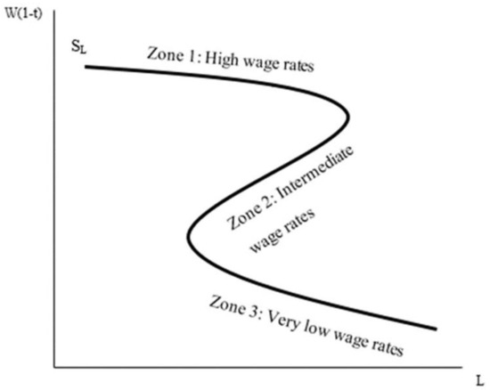
Figure 1.
Three zones of fluctuating labor supply.
Another aspect derived from the special inverted S-shaped labor supply curve concerns how it may influence the traditional one peak point of the Laffer curve. It appears that this aspect has never been considered by economists. The main purpose of the model developed below is to show that the S-shaped curve leads to a multi-peaked Laffer curve, or at least to a double-peaked S-shaped Laffer curve.
In the next section, the backward-bending labor supply curve is introduced, followed by an extension of the inverted S-shaped labor supply curve, due to subsistence income requirements. It is based on our specific utility function, which differs from the utility function used by Nakamura and Murayama [21] and Eisenhauer [11]. As a result, the unique double-peaked shape of the Laffer curve is derived. A numerical example illustrates the case of the S-shaped labor curve and its influences on the Laffer curve.
We conclude the literature review regarding the Laffer curve with some additional, and very new, works. Four of them are theoretical articles that investigate the Laffer model in general. Another three papers empirically apply some issues of the Laffer curve, as described below. All seven articles have been very recently published, beginning from 2020.
Some papers criticized different aspects of the classical Laffer theory of the 1970s. The following is a brief review.
Sanz-Sanz [50] claims that the classical and generally accepted Laffer curve does not adapt to reality, since it does not take into consideration the tax revenues of indirect taxes and social security tax.
Another criticism by Moloi and Marwala [51] is that the original Laffer curve does not include technological improvement and revenues. Production by robots increases revenues and production, without influencing direct income taxes.
On the other hand, in their recent paper, Nakajima and Takahashi [52] used the basic Laffer curve differently from reflecting the traditional relationship between tax rate and direct tax revenue, by extending it to the relationship between government assets income or output. When they applied the model to the U.S. economy, they found a reversed Laffer curve, with the shape of a U. Thus, as the governmental assets–output relationship increases, the income–output relationship of its assets at first grows, reaching a maximum. It then decreases, ending in negative values.
Another recent paper by Fuller [53] repeats the discussion of the relationship between the tax rate and the tax revenue and demonstrates it in Figure 1 on page 311. In this figure, the tax rate is plotted on the y axis and the tax revenue that is the dependent variable is on the X axis, as was done by Laffer [32]. Fuller expands the discussion of the Laffer curve and analyzes the effect of the tax rate on the tax revenue for the sake of the capital accumulation curve, where the peak point level of tax revenue guarantees the highest level of accumulated capital. (See [53]) Figure 3, p. 314.)
In contrast to Sanz-Sanz [50], the present paper focuses on the standard approach of analyzing the relationship between the tax rate of personal income and the total income tax revenue. This limited approach was not accepted by Sanz-Sanz. He believes that a change in the tax rate may have an effect on other taxes, such as consumption taxes, social security contributions, etc.
In recent years, additional empirical research has been conducted regarding the Laffer curve. This is illustrated in the following three articles: Wang et al. [54] investigated the optimal tax rate in the Visegrad Group (V4 countries), with data collected from 1995 to 2017. According to the research results, the Laffer curve reflects the general situation in those countries. Their research also shows that in Poland and the Slovak Republic, the determined tax rates result in optimal tax revenues, while Czech Republic and Hungary need to adjust their tax rates.
Ferreira-Lopes et al. [55] also empirically investigated the Laffer curve in every country in the Eurozone, using panel data from 1995 until 2011. Their primary result showed that a large gap exists between the optimal tax rates for the Eastern European countries and the economies of Western Europe.
A third research work, conducted by Germán-Soto [56], investigated whether the external debt–economic growth relationships in Mexico during the years 1970–2017 were like the Laffer curve. The result showed that Mexico needs to decrease its external debt burden, in order to renew the path of stable growth and be on the optimal path of the Laffer curve.
5. The Model
Let us begin by introducing the specific utility function that generates the inverted S-shaped labor supply curve, leading to a special double-peaked Laffer curve. The uniqueness of our analysis is that we use a specific combination of utility functions that generates the formal inverted S-shaped labor supply. First, we assume an additive separable utility function with respect to leisure and earned net income, from which we can generate a backward-bending labor supply. The labor supply is affected positively by the net wage rate at low and intermediate ranges. The function we use guarantees the range of wage rate in which the substitution effect is dominant and stronger than the income effect. At higher wage rates, the income effect of the specific additive utility function is positive and stronger than the substitution effect. Thus, an increase in the net wages encourages less labor supply, generating a backward-bending labor supply curve. This additive utility function, of both the normal goods, income, and leisure, exists at the normal labor supply range. However, at a very low net wage rate, the utility function changes and is completely unaffected by leisure, since very poor people desire a certain minimal income for survival, regardless of leisure. Thus, lower net wage requires more labor (i.e., less leisure). At this range, the labor supply curve is hyperbolic with respect to the net wage rate (see Equation (15) in the following section). As shown below, this specific utility function leads to multiple peaks of the Laffer curve.
In order to demonstrate the modified Laffer curve, we introduced mathematically combined utility functions that lead to this modification.
We use some specific utility functions that have been used by economists and apply them in the market of labor supply, indirectly affecting the Laffer curve.
We take a backward-bending supply curve derived from a quadratic mathematical function. We adopted this function from the early work of Hanoch [1], who generally discusses the backward-bending labor supply curve. We develop a specific mathematical utility function, in which income and substitution effects affect in opposite directions. The dominancy effect leads the labor supply to be negatively and/or positively sloped.
In addition, an additive utility function in relation to leisure and consumption is assumed. This enables creating a supply of labor that increases while the net wage decreases. This occurs at a certain low wage rate, and repeats; i.e., a decrease in the labor supply occurs in response to net wage increases. As a result, it generates a backward-bending supply of labor, as presented in Figure 2.
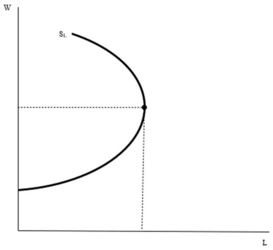
Figure 2.
The backward-bending labor supply curve.
This last supply curve function is combined with a third zone at a very low wage rate, where a further decrease in the wage rate increases the labor supply curve as a hyperbolic form function. The combination of the various zones of the labor supply leads to a specific Laffer curve with more than one peak point. This combination of two different utility functions, which may exist in reality, creates a fluctuating relationship between the tax rate and tax revenue.
The purpose of the following model is to develop a scientific method to challenge the conventional opinion of public economics experts, led by Arthur Laffer. Their approach is that the relationship between tax revenues and tax rates imposed on employees necessarily creates a bell-shaped curve that contains one peak point.
Let us discuss in detail the contradiction to the one peak point conclusion described above. In two different cases, the influence of the net wage rates generates fluctuations in opposite directions on the individual labor supply. In the first case, we find in a discussion by Yang [57]. He mentions the case in which leisure positively affects utility, since at a certain and intermediate range of the net wage rate, leisure is expected to be a normal and even a luxury good. In such a case, an increase in the net wage rate leads to an increase in leisure since the income effect is large and dominant, in comparison to the substitution effect. Thus, the labor supply increases in response to an increase in the net wage rate. However, at a very high or a very low net wage rate, leisure is considered by Yang [57] as a very inferior good, referred to as a Giffen good. In these cases, the combination of substitution and inferiority income effects leads to the following: An increase in the net wage rate encourages an increase in labor supply, due to the substitution effect. Since leisure is inferior, the net wage leads to a further increase in the labor supply. If, indeed, in an extreme case of very high and very low wage rates leisure is considered a very inferior good (Giffen good), the inverted labor supply has an S-shaped curve, as shown by Yang [57] in Figure 2 on page 46.
Our approach is totally different from that of Yang [57], although Yang’s approach leads to the same conclusion regarding the inverted S-shaped labor supply curve. We object to Yang’s approach, since we believe that inferiority characteristics are not relevant in the case of leisure items. The conventional approach, which was acceptable during the last century by most social scientists, considers leisure as a normal good or even a luxury good, but definitely not an inferior or a Giffen good. We differ from Yang [57] in using another explanation for the rotating supply curve, as used theoretically and empirically in several recent works mentioned above in the Introduction.
Based on specific utility functions that include a positive income effect on consumption and leisure, those works show ranges where an increase in the net wage rate increases the labor supply, since the substitution effect is dominant. However, as the wage rate is high enough, the supply of labor is negatively affected, due to the dominancy of the income effect on leisure. This leads to the backward-bending labor supply curve (Figure 1). However, at a significantly low wage rate in the economic and social environment, it may occur that a further reduction in the wage rate forces the worker to work more. This leads to another turning point of the labor supply, such that the labor supply curve has an inverted S-shape. As a result of this shape of the labor supply, we depart from the classical one peak point Laffer curve, as shown by Fève [27].
Let us introduce the relationship between the imposition of tax rate, t, on labor, L, and its effect on the tax revenue, T, as explained by Arthur Laffer and his followers. The Laffer curve describes the relationship between the independent variable, average tax rate, t; and the dependent variable, tax revenue, T, at a given gross wage rate, W. The curve is shown in Figure 3 and has been theoretically and empirically studied for more than 40 years.
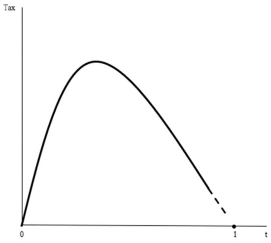
Figure 3.
The single-peaked Laffer curve.
Another case is examined, where the inverted S-shaped labor supply L [W, (1-t)] becomes negative sloped again when t is very high because the net wage rate W(1-t) is very low. It is evident from the equations above that the wage tax revenue, T= tWL, undoubtedly increases again with t. Hence, the Laffer curve may include a peak point as well as a bottom point, approaching another peak point. This will be shown in the model we develop below. However, depending on t/(1-t) and ε, even under a conventional backward-bending labor supply, the sign of ∂T/ ∂t is ambiguous, when t is high or the net wage rate W(1-t) is low.
Using a specific utility function, sufficient conditions are developed below to demonstrate the multi-peak feature of the Laffer curve.
The case of the backward-bending labor supply curve assumes a consumer whose utility, U, is affected positively by income, I, earned from working daily hours and by daily hours of leisure, where = .
The utility function in Equation (1) is based on the framework that economists typically use to analyze labor supply behavior. During the last decades, it has been used and referred to as the neoclassical model of the choice between labor and leisure; see, for example, a recent book entitled Labor Economics by Professor Borjas from Harvard University [58].
This neoclassical approach is applied in a paper by Spiegel and Templeman [12] to a very specific utility function that is additive and has two characteristics. While the marginal utility of consumption is constant, the marginal utility of leisure is diminishing.
This specific utility function, U, in Equation (1) that is used by Spiegel and Templeman [12] results in the backward-bending labor supply curve, as follows:
where are defined as three positive values parameters.
The objective of the representative consumer is to maximize the utility presented in Equation (1), subject to the budget constraint in Equation (2) below.
where t is the (average) tax rate. Thus, is the net wage rate for each working hour of the consumer.
To avoid a corner solution, i.e., to guarantee positive values of and , Equation (3) is required to hold at equilibrium:
where measures the marginal utility of another unit of leisure time and measures the marginal utility of additional dollar income that is spent by the consumer.
At equilibrium the marginal rate of substitution (MRS):
where at equilibrium the budget constraint tangent to the indifference curve.
Thus,
This indicates that in our specific utility function, the marginal utility of a unit of leisure is equal to the marginal utility of additional dollar income spending.
The second requirement presenting at Equation (6) is:
or
or
From (4) we get
or
From (10) and (2) we get (11)
where L is the labor supply function that generates several zones of the labor supply curve as a function of the net wage rate as follows.
The influence of changes in the net wage rate on labor supply is presented below:
Equation (12) can be divided into different zones:
Zone 1. At reservation net wage rate of and below that value, the labor supply is zero. Therefore the tax revenue, T, is zero. See point K in Figure 4 for a given
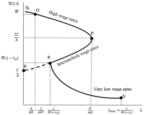
Figure 4.
The inverted S-shaped labor supply curve.
Zone 2. At the range of net wage where the backward-bending supply curve exists. There is a negative effect of the net wage rate on the labor supply, since the income effect is dominant. In this case, an increase in the tax rate also leads to an increase in labor supply and, therefore, the tax revenue increases exponentially. Later on the substitution effect is dominant, but the labor supply still increases by a lower percentage than the percentage increase in the tax rates. Therefore, tax revenue continues to increase up to point P (peak point of the Laffer curve). This occurs at Zone 3, where at the net wage rate of , the labor supplied is affected positively by the net wage rate on the labor supply curve, due to the dominant substitution effect. At some point, the percentage increase in the tax rate is smaller than the percentage reduction in the labor supply. Therefore, the tax revenue decreases by the tax rate increase up to point R, (Zone 3 between points P (Peak) and R (Minimum)).
The influences of the tax rate, t, and the tax revenue based on the inverted S-shaped labor supply curve are presented in Figure 5 below.
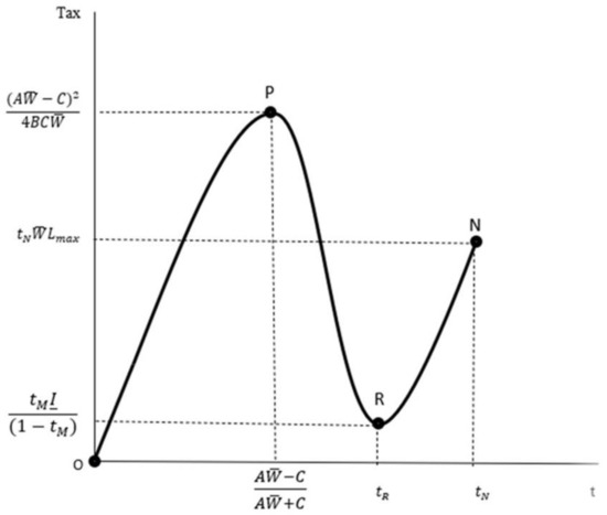
Figure 5.
The Laffer curve in the case of the inverted S-shaped labor supply curve.
We start with the discussion of the Zone, between points R and N in Figure 5 of the Laffer curve, as well as in Figure 4.
The following discussion analyzes the shape of another range of the labor supply curve, which maintains subsistence net income, .
Figure 4 demonstrates the case of the S-shaped curve that is discussed by Sharif and others, mentioned above [4,5,6,7,8,9,10,11], with regard to an additional zone of the inverted S-shaped labor supply curve. The curve fluctuates with changes in the net wage rate, , and creates three zones at a high net wage rate. The income effect leads to less labor supply when the net wage is higher. In another zone of lower net wage rate, due to dominance of the substitution effect, a higher net wage rate increases labor supply.
However, due to subsistence net income theory, at a significantly low net wage rate, which may occur at a high tax rate, the worker is required to supply more labor to guarantee a certain subsistence income, . This occurs in zone RN in Figure 4, as explained below.
We define the value in Figure 4, above, at point R where:
For a given , there are several combinations of and labor supply values that guarantee net income of, , at the range along this curve RN, as given at (14).
The negatively sloped curve at range RN requires a percentage decrease in the quantity of labor supplied, which is similar to the percentage increase in the value of This condition guarantees a given net subsistence income, , at different combinations of and .
These special shapes of the labor supply, which fluctuates with changes in the wage rate, lead to an inverted S-shaped curve that is similar to the results presented by Eisenhauer [11], derived from the Friedman–Savage [37] utility function. A similar shape of labor supply is presented by Nakamura and Murayama [21] in Figure 5 on page 673. That figure is similar to our Figure 4 below.
The formal inverted S-shaped labor supply curve below is:
The Derivation of the Laffer Curve in the Case of the Inverted S-Shaped Labor Supply Curve
At this stage of the model, another question that should be discussed is how the Laffer curve is derived, if indeed the labor supply fluctuates and has an S-shaped curve. The Laffer curve that is written as tax revenue, Taxi, which is affected by tax rate, ti, for a given gross wage rate, is:
From (13) it is clear that three zones of the Laffer curve exist.
At the zone in which then
At the zone in which then
The last zone of the Laffer curve is the zone RN of the labor supply that should guarantee subsistence net income. This is a little more complicated, and is discussed below.
At this zone of RN of the labor supply, the gross income, GI, is for any level of labor supply , defined as:
From (14) the substance income is given. Thus, the difference between (14) and (19) measures the tax revenue of (20) in zone RN, as follows:
Since the value of net subsistence income is measured at (14) while (19) represents the gross income, the differences between (14) and (19) measure the tax revenue of (20) at zone RN.
Thus,
or
and
Therefore, the Laffer curve at zone RN of the S-shaped curve is:
when .
Based on the discussion, above, the formal Laffer curve Tax = f(ti) that ‘covers’ the three zones is:
These zones of the Laffer curve are presented in Figure 5 and also discussed in Appendix A.
The figure presents a different shape of Laffer curve. Instead of the original Laffer curve, with one peak (as in point P in Figure 5), the Laffer curve that is derived from the inverted S-shaped labor supply curve contains another peak point of tax revenue at a high tax rate, tN (See point N in Figure 5).
The curve is not multi-peaked but double-peaked, with one bottom point. Another peak point of the tax revenue exists at point N in Figure 5. This is due to the fact that along the region between R and N, an increase in the tax rate leads to an increase in the labor supply. Thus, revenue increases by an increasing rate. Beyond this point, an additional increase in the tax rate represents entering into the subsistence income level. Therefore, the worker disconnects himself from the labor market and prefers self-production, which enables him to survive, while also avoiding any taxation. Self-production is tax free. In such a case, the tax revenue definitely drops very significantly. This evidence justifies our claim that point N is a local peak point.
6. Welfare Implications and the Unique Shape of the Laffer Curve
This section discusses the welfare implications that are derived from the inverted S-shaped labor supply, which influences the shape of the Laffer curve. In the Laffer curves that have been presented by most economists, the classical and traditional shape of one peak point is based on the following assumption: At a given high gross wage rate, an increase in the tax rates increases the tax revenue up to a certain peak point. Further increase in the tax rate reduces tax revenue. However, from the perspective of efficiency, policymakers do not choose a further increase of the tax rate. The lower tax rate that guarantees the same tax revenue is preferable.
However, the present consideration is with regard to the case in which the original basic gross wage rate is, relatively, very low. In this case, it is possible that the Laffer curve increases with any increase of the tax rate. It is even possible to approach the positive slope of the labor supply. A simultaneous increase in the tax rate and the labor supply causes the Laffer curve to increase at an increasing rate with the same tax rate, toward another peak point of the Laffer curve.
The preceding discussion raises the conflict between the desire of the policymaker to gain more tax revenue by increasing the tax rate, and the resulting imposition of a tax burden on the welfare of workers. This conflict is crucial, especially for workers whose gross wage rate is very low and who have a subsistence standard of living. The trade-off that the policymaker faces between collecting revenues and imposing a higher tax burden on customers, some of whom are very poor, departs from the standard analysis of the Laffer curve. The classical approach to the Laffer curve is usually very neutral and raises only the issue of tax effectiveness and efficiency. The extension of the inverted S-shaped labor supply curve also includes the aspects of poor, non-professional, and unqualified workers. (For example, see the case of the tourism industry discussed above). This emphasizes that the issues of fairness and inequality should be considered by policymakers regarding the desirable and appropriate tax rates that should be imposed for the sake of tax revenues. The lower tax rate that guarantees a given tax revenue is preferable from an efficiency and fairness perspective. Moreover, it is possible that for any given gross wage rate the policymaker may impose a very high tax rate. This may lead to so low a net wage rate that it is already defined within the range of subsistence income. In such a case, the imposition of a higher tax rate would force the worker to work more hours to reach a minimum net income, for the sake of survival. Therefore, a combination of more labor hours with a higher tax rate definitely leads to an increase of tax revenue, i.e., an increase in the Laffer curve towards another peak. This possibility leads to the case of collecting a certain tax revenue at three different tax rates. Again, the lowest tax rate of the three will be chosen by the policymaker, due to effectiveness and efficiency. Based on our analysis and the modification that has been made, the important conclusion is that the Laffer curve does not necessarily maintain a global maximum as a single peak point that can fluctuate several times with more than one turning point. Mathematically we may say that the real Laffer curve has several local maximum and minimum points.
However, the present consideration is with regard to the case in which the original basic gross wage rate is, relatively, very low. In this case, it is possible that the Laffer curve increases with an increase in the tax rate. It is even possible to approach a positive slope of the labor supply. A simultaneous increase in the tax rate and the labor supply causes the Laffer curve to increase at an increasing rate with the tax rate.
This last case raises the conflict between the desire of the policymaker to gain more tax revenue by increasing the tax rate and the resulting imposition of a tax burden on the welfare of workers. Especially affected are workers whose basic gross wage rate is very low and for whom a subsistence standard of living is required. The trade-off that the policymaker faces, between collecting revenues and imposing a burden on customers, some of whom are very poor, departs from the standard analysis of the Laffer curve and was not originally considered at all by Laffer himself. The classical approach to the Laffer curve is usually very neutral and raises only the issue of tax effectiveness. The extension of presenting the inverted S-shaped labor supply curve analysis also includes the aspects of poor, non-professional, and unqualified workers. For example, see the case of the tourism industry discussed above. This requires discussion of the issues of fairness and inequality, which should be considered by policymakers regarding the desirable and appropriate tax rates imposed for the sake of tax revenues.
At this stage, we introduce additional aspects of the preceding discussion. Fluctuations in the shape of the labor supply generate a new Laffer curve. Instead of a classical bell-shaped curve, with one peak point, a modified Laffer curve exists, with more than one peak point. In addition to efficiency and effectiveness, the modified shape of the Laffer curve reflects other elements, such as equality and fairness, which should be considered with regard to the issue of the tax burden.
The original Laffer curve analysis includes the possibility of one peak point, where tax revenue is achieved at a global optimum. Another result is derived, since any tax revenue can be achieved by the low and high tax rates. The lower tax rate should be chosen by a policymaker, since the lower tax rate generates a smaller tax burden. While the lower tax rate is more effective (less tax burden), it is also less equitable, because relatively more tax burden is imposed on the poor.
The scenario of a multi-peaked curve (not necessarily two points) represents the conflict between tax effectiveness, and fairness and equality. Fluctuations between tax revenues and tax rates raise the following conflicts: Different tax rates with the same tax revenues may bring very high tax revenues that are imposed on the rich, while the poor workers with low wages do not gain a net wage after high tax imposition. Thus, the tax is most likely imposed on the rich. This issue of deficiency of taxes is not relevant in the case of the classical Laffer curve with one peak point.
Another important implication of our current paper is the conclusion that knowing the actual level of tax revenue, as well as the actual tax rate, is reliable information for making decisions such as raising or reducing the tax rate while knowing the one peak tax revenue. Our results enable multiple peak points of the modified Laffer curve, question the reliability of the whole curve, and raise doubts concerning its usefulness. Different shapes of the S-shaped labor supply of different workers, and different distributions of gross wages of given populations may cause economists and policymakers to doubt the ‘belief’ of many others regarding the usefulness of the classical Laffer curve.
Author Contributions
Conceptualization, L.D.G. and T.T. and U.S.; methodology, L.D.G. and T.T. and U.S.; validation, L.D.G. and T.T. and U.S.; formal analysis, L.D.G. and T.T. and U.S.; investigation, L.D.G. and T.T. and U.S.; writing—original draft preparation, L.D.G. and T.T. and U.S. writing—review and editing, L.D.G. and T.T. and U.S.; visualization, L.D.G. and T.T. and U.S.; supervision, U.S.; project administration, U.S. All authors have read and agreed to the published version of the manuscript.
Funding
This research received no external funding.
Institutional Review Board Statement
Not applicable.
Informed Consent Statement
Not applicable.
Data Availability Statement
Not applicable.
Conflicts of Interest
The authors declare no conflict of interest.
Appendix A
The Laffer curve of the two zones should be discussed. At the origin point at which the tax rate, ti, is zero, the total tax revenue is also zero. At a positive tax rate, the tax revenue is positive, and an increase in the tax rate leads to an increase in the labor supply. Thus, the total tax revenue is increasing. Therefore, the Laffer curve is:
Let us examine the effect of an increase in the tax rate of the tax revenue implementing Equation (11) into (A1) and taking the derivative:
At a certain value of equals zero. This occurs when (A3) holds:
(A3) exists if the tax rate is
By implementing (A4) at (A1) we get a tax revenue that is at maximum and equal to the term below:
To guaranteed maximization of tax revenue, the second order condition exists as shown below at (A6):
Since the value in the brackets at (A6) is zero and the second term of the equation is negative, the tax revenue is at maximum for t*.
References
- Hanoch, G. The “Backward-bending” Supply of Labor. J. Political Econ. 1965, 73, 636–642. [Google Scholar] [CrossRef]
- Varian, H.R. Intermediate Microeconomics with Calculus: A Modern Approach, 8th ed.; Repcheck, J., Ed.; W.W. Norton & Company: New York, NY, USA, 2013. [Google Scholar]
- Nicholson, W.; Snyder, C.M. Intermediate Microeconomics and Its Applications, 11th ed.; Kindle Edition; Cengage Learning: Boston, MA, USA, 2009. [Google Scholar]
- Sharif, M. The concept and measurement of subsistence: A survey of the literature. World Dev. 1986, 14, 555–577. [Google Scholar] [CrossRef]
- Sharif, M. Poverty and the forwards-falling labor supply function: A microeconomic analysis. World Dev. 1991, 19, 1075–1093. [Google Scholar] [CrossRef]
- Sharif, M. Inverted “S”, the complete neo-classical labour-supply function. Int. Labour Rev. 2000, 139, 409–435. [Google Scholar] [CrossRef]
- Dessing, M. Implications for minimum-wage policies of an S-shaped labor–supply curve. J. Econ. Behav. Org. 2004, 53, 543–568. [Google Scholar] [CrossRef]
- Barzel, Y.; McDonald, R.J. Assets, Subsistence, and The Supply Curve of Labor. Am. Econ. Rev. 1973, 63, 621–633. [Google Scholar]
- Lin, C.-C. A backward-bending labor supply curve without an income effect. Oxf. Econ. Pap. 2003, 55, 336–343. [Google Scholar] [CrossRef][Green Version]
- Riley, M.; Szivas, E. The valuation of skill and the configuration of HRM. Tour. Econ. 2009, 15, 105–120. [Google Scholar] [CrossRef]
- Eisenhauer, J.G. Labor supply with Friedman-Savage preferences. Stud. Econ. Finance. 2014, 31, 186–201. [Google Scholar] [CrossRef]
- Spiegel, U.; Templeman, J. A non-singular peaked Laffer Curve: Debunking the traditional Laffer Curve. Am. Econ. 2004, 48, 61–66. [Google Scholar] [CrossRef]
- Tavor, T.; Gonen, L.D.; Spiegel, U. Reservations on the classical Laffer curve. Rev. Austrian Econ. 2019, 34, 479–493. [Google Scholar] [CrossRef]
- Hussain, M.; Saud, A.; Khattak, M.U.R. Socio-Economic Determinants of Working Children: Evidence from Capital Territory of Islamabad, Pakistan. Pak. Adm. Rev. 2019, 1, 145–158. [Google Scholar]
- Luckstead, J.; Tsiboe, F.; Nalley, L.L. Estimating the economic incentives necessary for eliminating child labor in Ghanaian cocoa production. PLoS ONE 2019, 14, e0217230. [Google Scholar] [CrossRef]
- Masud, R.M. Tourism as a livelihood development strategy: A study of Tarapith Temple Town, West Bengal. Asia-Pacifc J. Reg. Sci. 2020, 4, 795–807. [Google Scholar]
- Nguyen, T.T.M.; Don, R.R.; Clifford, J.S., II. Tourism as Catalyst for Quality of Life in Transitioning Subsistence Marketplaces: Perspectives from Ha Long, Vietnam. J. Macromarketing 2014, 34, 28–44. [Google Scholar]
- Mathew, S.S. Distress-Driven Employment and Feminisation of Work in Kasargod District, Kerala. Econ. Political Wkly. 2012, 47, 65–73. [Google Scholar]
- Dessing, M. Labor supply, the family, and poverty: The S-shaped labor supply curve. J. Econ. Behav. Organ. 2002, 49, 433–458. [Google Scholar] [CrossRef]
- Dessing, M. The S-shaped labor supply schedule: The evidence from LDCs. Can. J. Dev. Stud. 2007, 28, 63–104. [Google Scholar] [CrossRef]
- Nakamura, T.; Murayama, Y. A Compete Characterization of the Inverted S-Shaped Labor Supply Curve. Metroeconomica 2010, 61, 665–675. [Google Scholar] [CrossRef]
- Lundberg, S. The Added Worker Effect: A Reappraisal; Working Paper No 706; National Bureau of Economic Research: Cambridge, UK, 1981. [Google Scholar]
- Lundberg, S. The Added Worker Effect. J. Labour Econ. 1985, 3, 11–37. [Google Scholar] [CrossRef]
- Maloney, T. Employment Constraints and the Labour Supply of Married Women: A Re-examination of the Added Worker Effect. J. Hum. Resour. 1987, 22, 51–61. [Google Scholar] [CrossRef]
- Gärtner, D.L.; Gärtner, M. Wage traps as a cause of illiteracy, child labor, and extreme poverty. Res. Econ. 2011, 65, 232–242. [Google Scholar] [CrossRef]
- Song, H.; Dwyer, L.; Li, G.; Cao, Z. Tourism Economics Research: A Review and Assessment. Ann. Tour. Res. 2012, 39, 1653–1682. [Google Scholar] [CrossRef]
- Fève, P.; Matheron, J.; Sahuc, J.-G. The Horizontally S-Shaped Laffer Curve. J. Eur. Econ. Assoc. 2018, 16, 857–893. [Google Scholar] [CrossRef]
- Boqiang, L.; Zhijie, J. Tax rate, government revenue and economic performance: A perspective of Laffer curve. China Econ. Rev. 2019, 56, 1. [Google Scholar]
- Sanz-Sanz, J.F. The Laffer curve in schedular multi-rate income taxes with non-genuine allowances: An application to Spain. Econ. Model. 2016, 55, 42–56. [Google Scholar] [CrossRef]
- Şen, H.; Bulut-Çevik, Z.B.; Kaya, A. The Khaldûn−Laffer Curve Revisited: A Personal Income Tax−Based Analysis for Turkey. Transylv. Rev. Adm. Sci. 2019, 15, 103–118. [Google Scholar] [CrossRef]
- Laffer, A.B. Government Exactions and Revenue Deficiencies. Cato J. 1981, 1, 1–21. [Google Scholar]
- Laffer, A.B. The Laffer Curve: Past, Present, and Future.; Executive Summary Backgrounder; The Heritage Foundation: Washington, DC, USA, 2004; p. 1765. [Google Scholar]
- Fullerton, D. On the Possibility of an Inverse Relationship between Tax Rates and Government Revenues. J. Public Econ. 1982, 19, 3–22. [Google Scholar] [CrossRef][Green Version]
- van Ravestein, A.; Vijlbrief, H. Welfare Cost of Higher Tax Rates: An Empirical Laffer Curve for the Netherlands. Economist 1988, 136, 205–219. [Google Scholar] [CrossRef]
- Hsing, Y. Estimating the Laffer Curve and Policy Implications. J. Socio-Econ. 1996, 25, 395–401. [Google Scholar] [CrossRef]
- Smith, A. An Inquiry into the Nature and Causes of the Wealth of Nations; Atlantic Publishers & Distributors Ltd.: New Delhi, India, 2008; p. 1776. [Google Scholar]
- Friedman, M.; Savage, L.J. The utility analysis of choices involving risk. J. Political Econ. 1948, 56, 279–304. [Google Scholar] [CrossRef]
- Satriawan, E.; Ghifari, A.T. How does Parental Income Affect Child Labor Supply? Evidence From the Indonesian Family Life Survey; TNP2K Working Paper 2; Australian Government: Canberra, Australia, 2018. [Google Scholar]
- Walker, S.; Bartlett, A. Agency in Child Labor Decisions: Evidence from Kenya. 2018. Available online: http://barrett.dyson.cornell.edu/NEUDC/paper_11.pdf (accessed on 13 February 2022).
- Bendewald, J. Subsistence Theory in the U.S. Context: A Cross-Sectional Labor Supply Estimate. Economics Honors Projects. 2008, p. 7. Available online: https://digitalcommons.macalester.edu/economics_honors_projects/7 (accessed on 13 February 2022).
- Sharif, M. A behavioural analysis of the subsistence standard of living. Camb. J. Econ. 2003, 27, 191–207. [Google Scholar] [CrossRef]
- Sasmal, J.; Sasmal, R. Economic Growth, Structural Change and Decline of Child Labour in Agriculture: A Theoretical Perspective. In Child Labor in the Developing World; Posso, A., Ed.; Palgrave Macmillan: Singapore, 2020. [Google Scholar]
- Sasmal, J.; Guillen, J. Poverty, Educational Failure and Child Labour Trap: The Indian Experience. Glob. Bus. Rev. 2015, 16, 270–280. [Google Scholar] [CrossRef]
- El-Mallakh, N.; Maurel, M.; Speciale, B. Arab spring protests and women’s labor market outcomes: Evidence from the Egyptian revolution. J. Comp. Econ. 2018, 46, 656–682. [Google Scholar] [CrossRef]
- El-Mallakh, N.; Maurel, M.; Speciale, B. Women and Political Change: Evidence from the Egyptian Revolution; Working Papers P116; FERDI: Argyle, TX, USA, 2014. [Google Scholar]
- Kuépié, M. Child labor in Mali: A consequence of adults’ low returns to education? Educ. Econ. 2018, 26, 647–661. [Google Scholar] [CrossRef]
- Kumar De, U. Sustainable Nature-based Tourism, Involvement of Indigenous Women and Development: A Case of North-East India. Tour. Recreat. Res. 2013, 38, 311–324. [Google Scholar]
- Mings, R.C. The Importance of More Research on the Impacts of Tourism. Ann. Tour. Res. 1978, 5, 340–344. [Google Scholar] [CrossRef]
- Wilkinson, P.F. Strategies of Tourism in Island Microstates. Ann. Tour. Res. 1989, 6, 153–177. [Google Scholar] [CrossRef]
- Sanz-Sanz, J.-F. A full-fledged analytical model for the Laffer curve in personal income taxation. Econ. Anal. Policy 2020, 73, 795–811. [Google Scholar]
- Moloi, T.; Marwala, T. Artificial Intelligence in Economics and Finance. In Theories Advanced Information and Knowledge Processing; Springer Nature: Basel, Switzerland, 2020; Volume 7, pp. 63–70. [Google Scholar]
- Nakajima, T.; Takahashi, S. Uninsured idiosyncratic risk and the government asset Laffer curve. J. Macroecon. 2022, 71. [Google Scholar] [CrossRef]
- Fuller, E.W. A Critique of the Laffer Curve. Procesos Merc. Rev. Eur. Econ. Política 2020, 17, 311–316. [Google Scholar] [CrossRef]
- Wang, L.; Rousek, P.; Hašková, S. Laffer curve-a comparative study across the V4 (Visegrad) countries. Entrep. Sustain. Issues 2021, 9, 433. [Google Scholar] [CrossRef]
- Ferreira-Lopes, A.; Martins, L.F.; Espanhol, R. The relationship between tax rates and tax revenues in eurozone member countries-exploring the Laffer curve. Bull. Econ. Res. 2020, 72, 121–145. [Google Scholar] [CrossRef]
- Germán-Soto, V. The Laffer Curve in the External Debt-Economic Growth Relationship in Mexico, 1970–2017. Rev. Mex. Econ. Finanzas 2020, 15, 205–225. [Google Scholar]
- Yang, B. The Analysis of the Impacts of China’s Personal Income Tax System on Labor Supply of Urban Dweller. Can. Soc. Sci. 2019, 15, 45–49. [Google Scholar]
- Borjas, G. Labor Economics; McGraw-Hill: New York, NY, USA, 2010. [Google Scholar]
Publisher’s Note: MDPI stays neutral with regard to jurisdictional claims in published maps and institutional affiliations. |
© 2022 by the authors. Licensee MDPI, Basel, Switzerland. This article is an open access article distributed under the terms and conditions of the Creative Commons Attribution (CC BY) license (https://creativecommons.org/licenses/by/4.0/).