
Fractional Growth Model with Delay for Recurrent Outbreaks Applied to COVID-19 Data

 ,
,  ,
,  , and
, and
Abstract
:1. Introduction
2. Mathematical Preliminaries
2.1. Fractional Calculus
- Fractional integral applied to a polynomial had the following analytic expression:
- If then and .
- The fractional derivative of Caputo and the fractional integral behave as inverse operators, as follows:
- If the order of the operators is interchanged, one mustand
2.2. Delayed Fractional Differential Equations
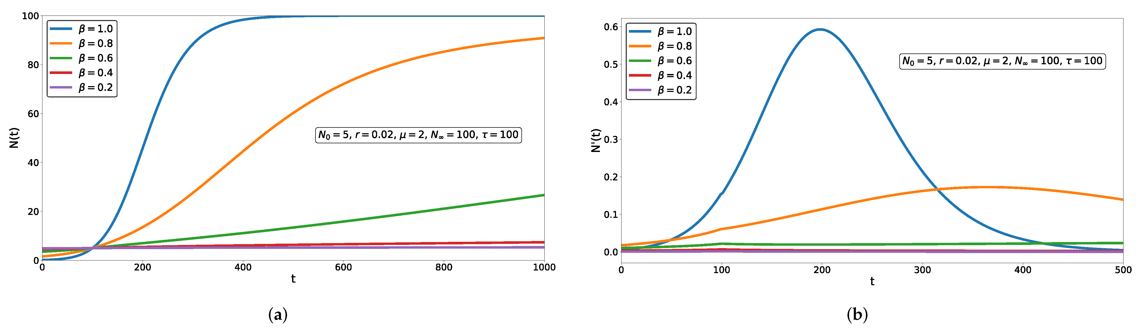
3. Fractional Growth Model with Delay
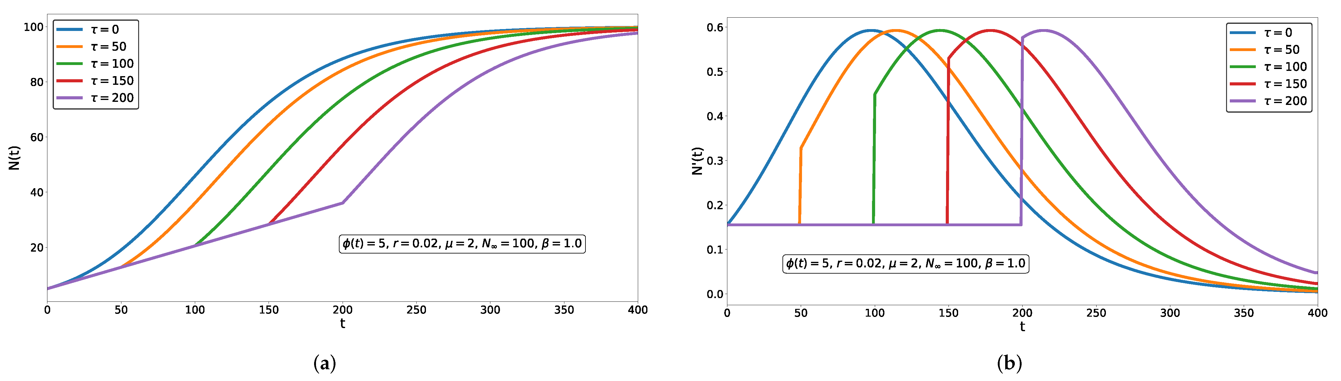
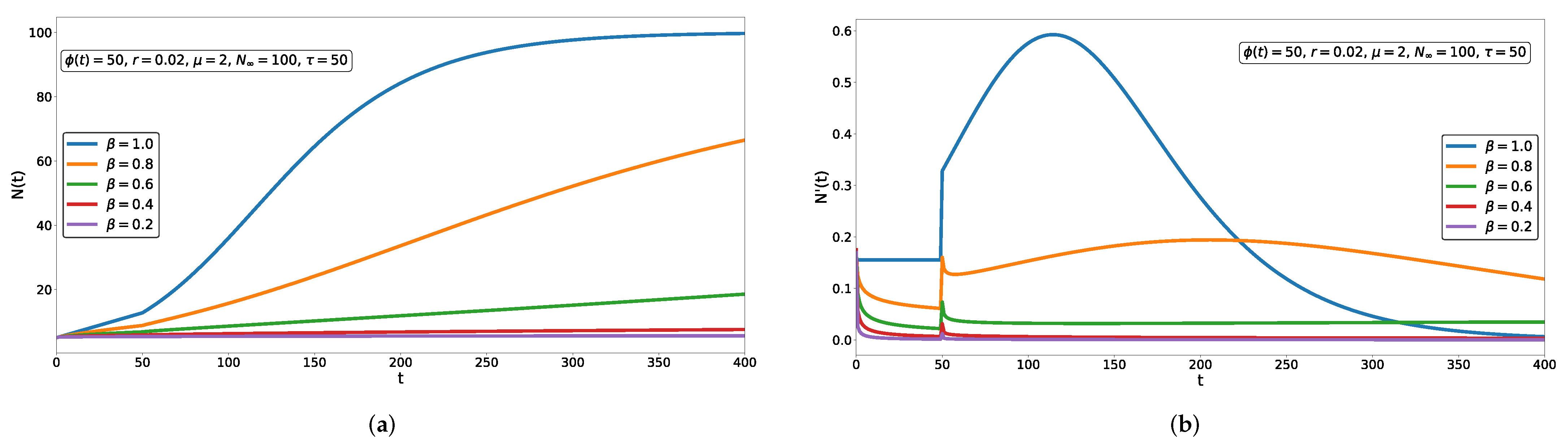
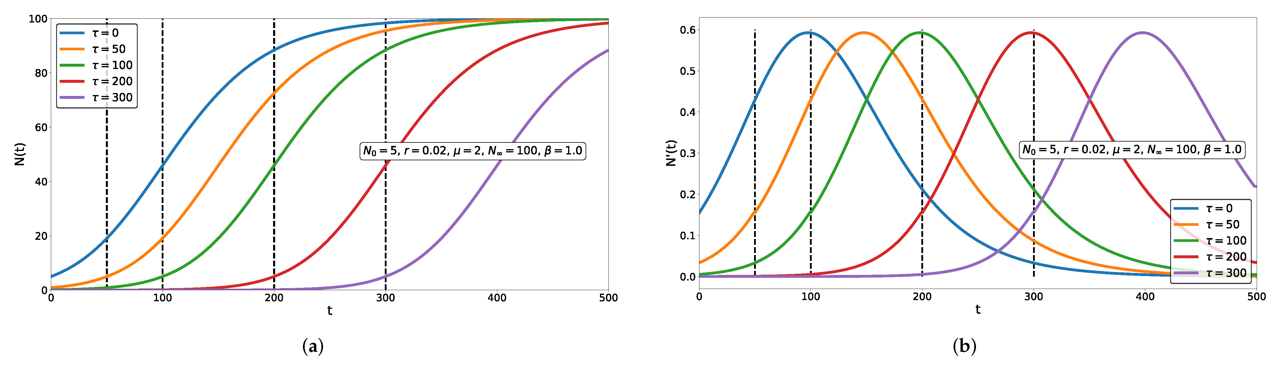
3.1. Sensitivity Analysis and Delay Effect
3.2. Initial Function Construction
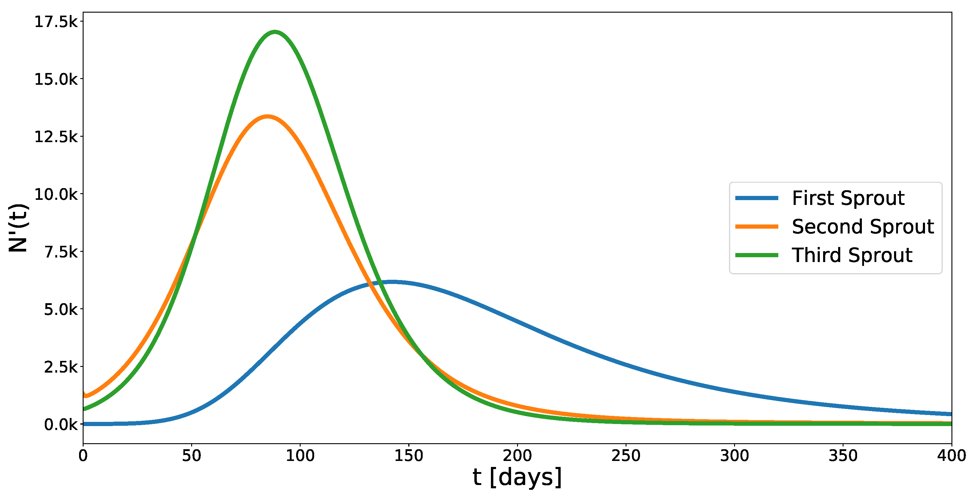
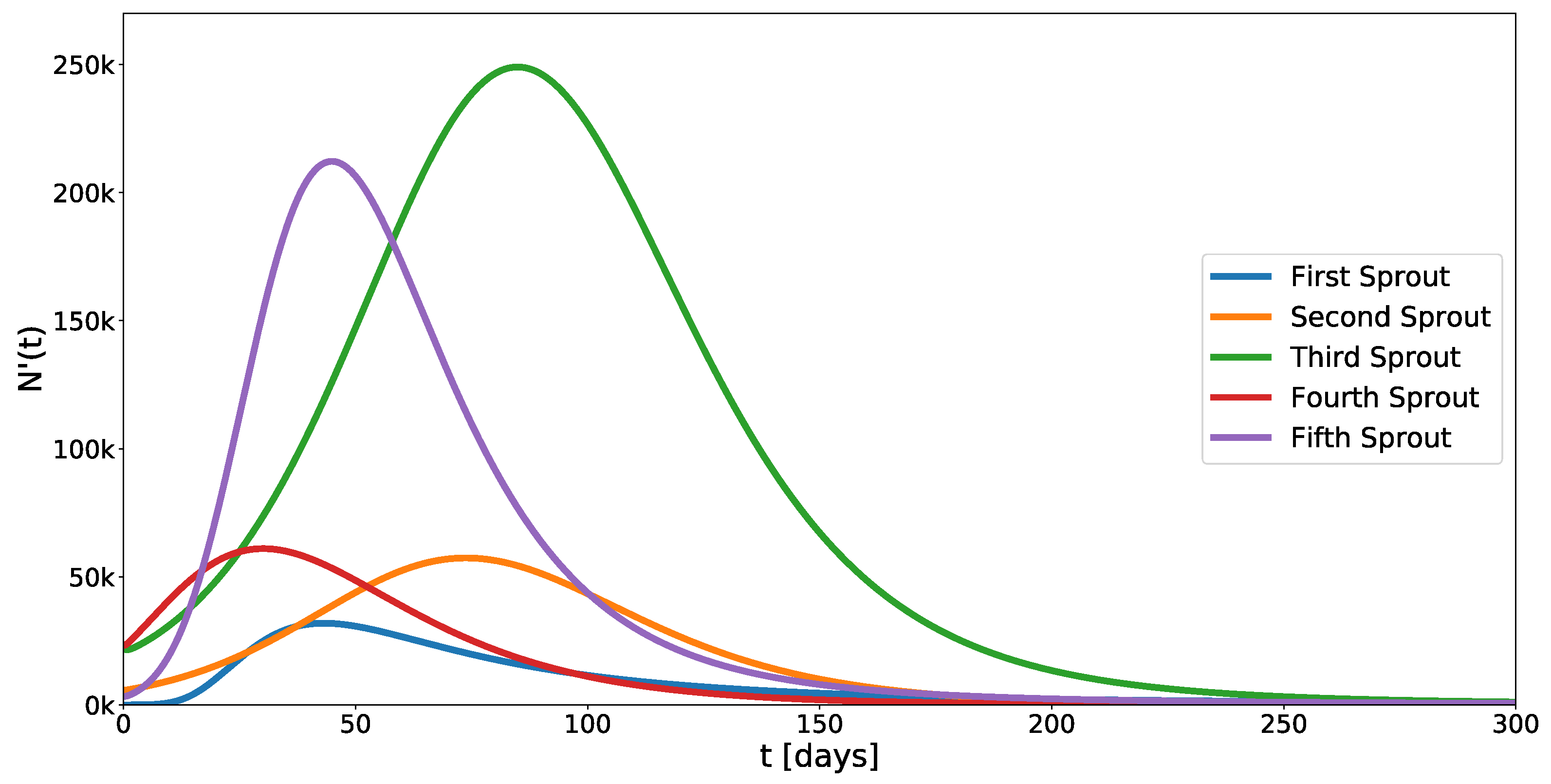
4. Fractional Growth Model with Delay for Recurrent Outbreaks
5. Applications to COVID-19 Data
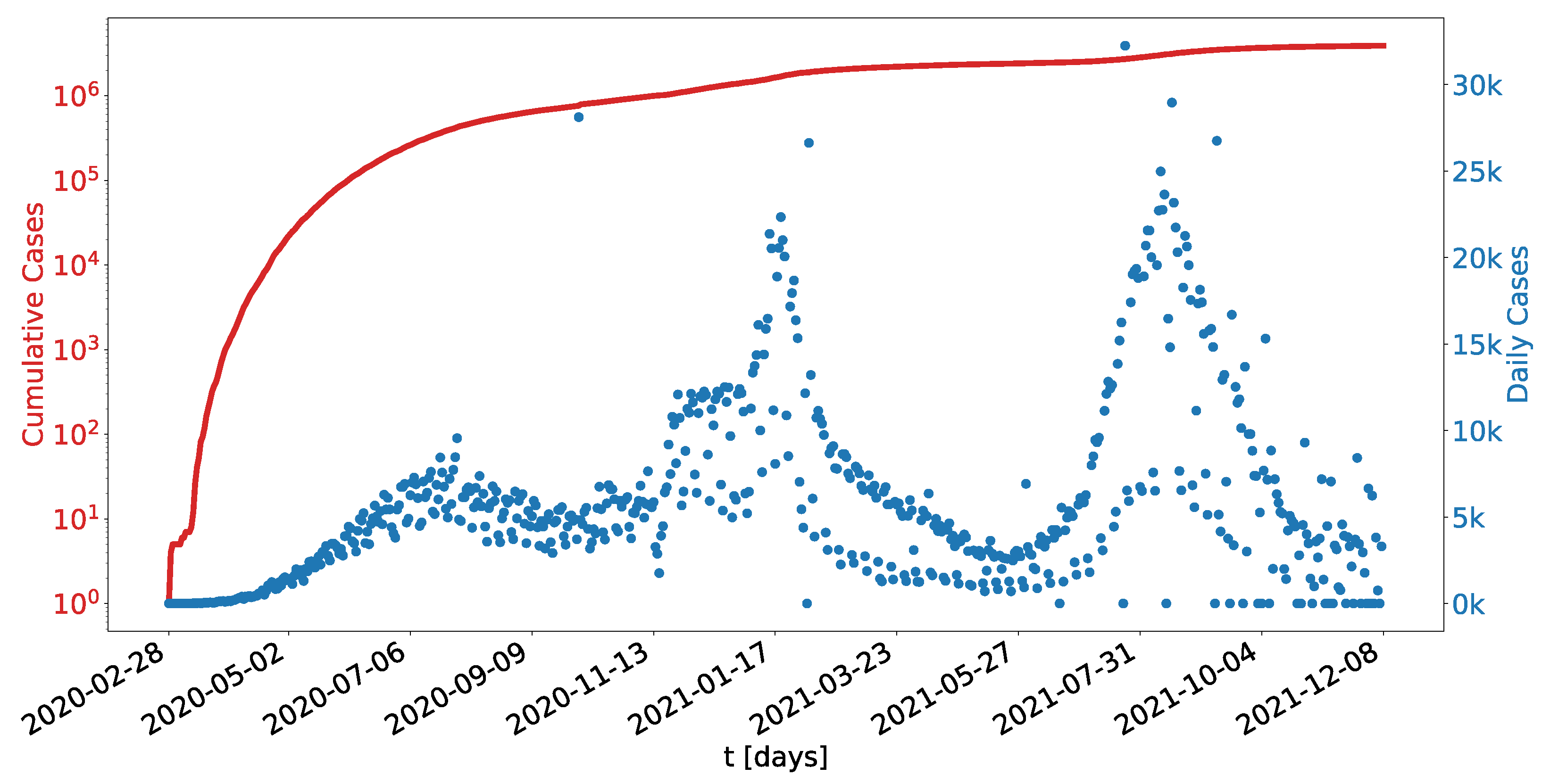
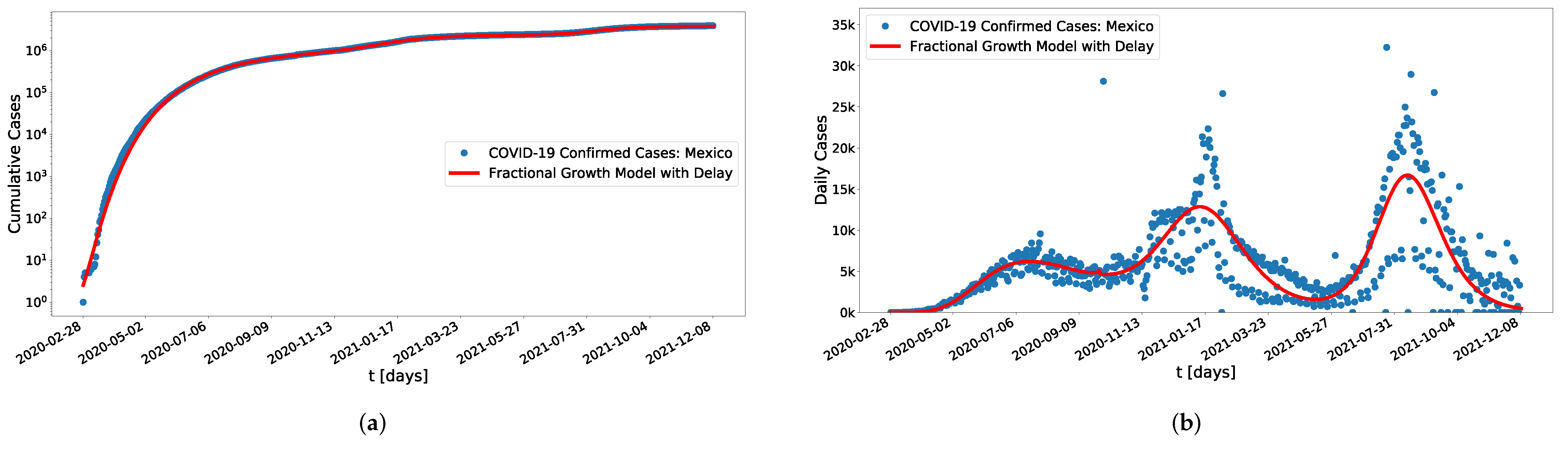
5.1. Mexico Data
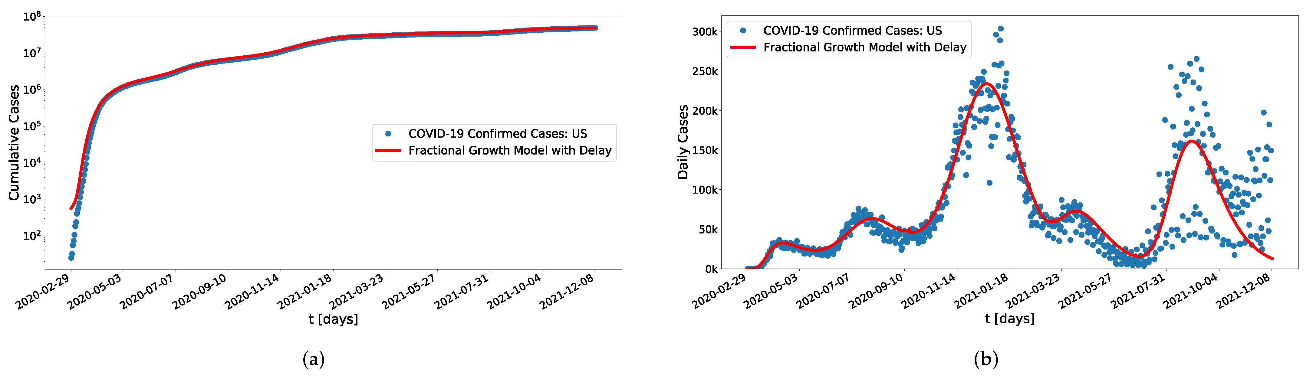
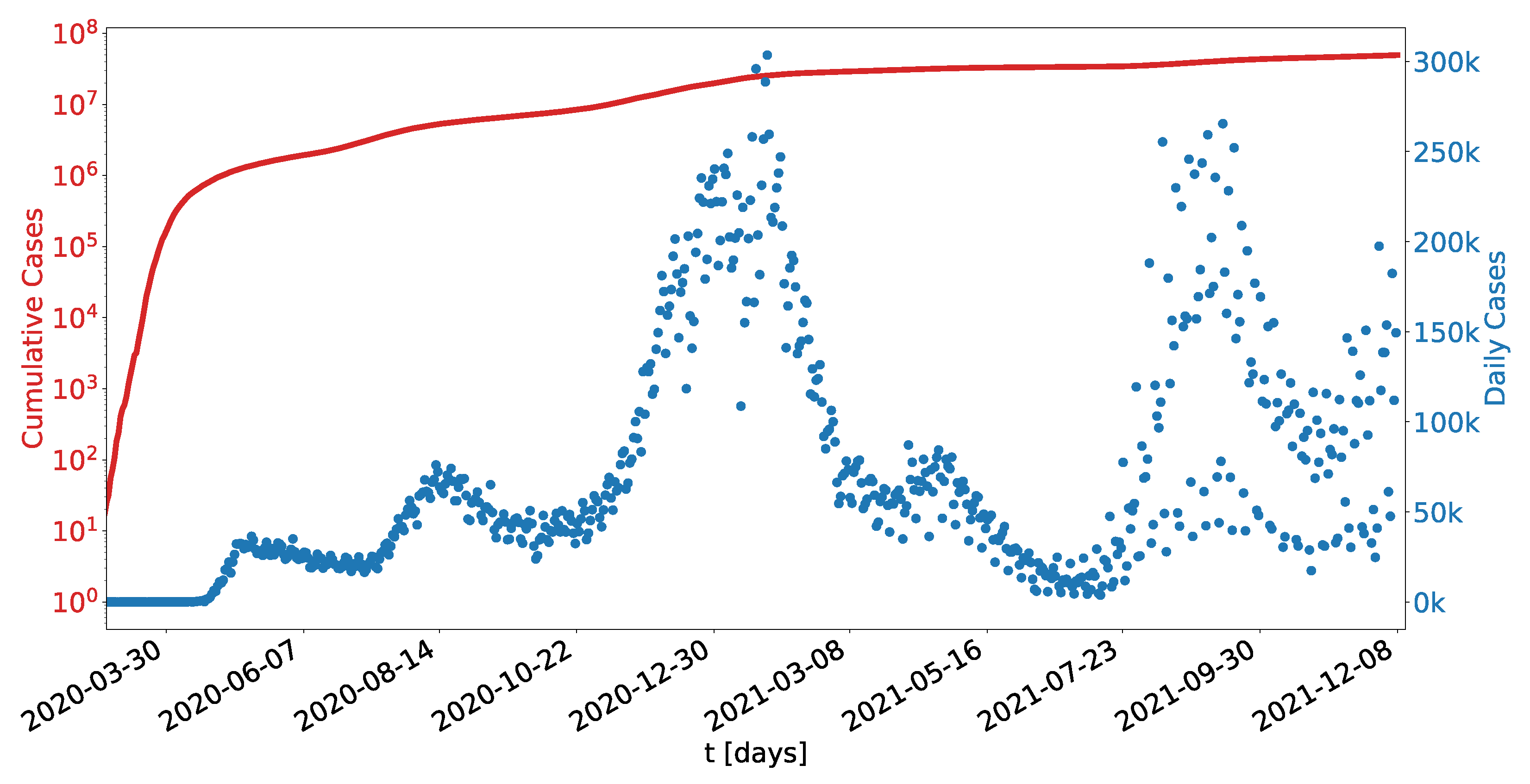
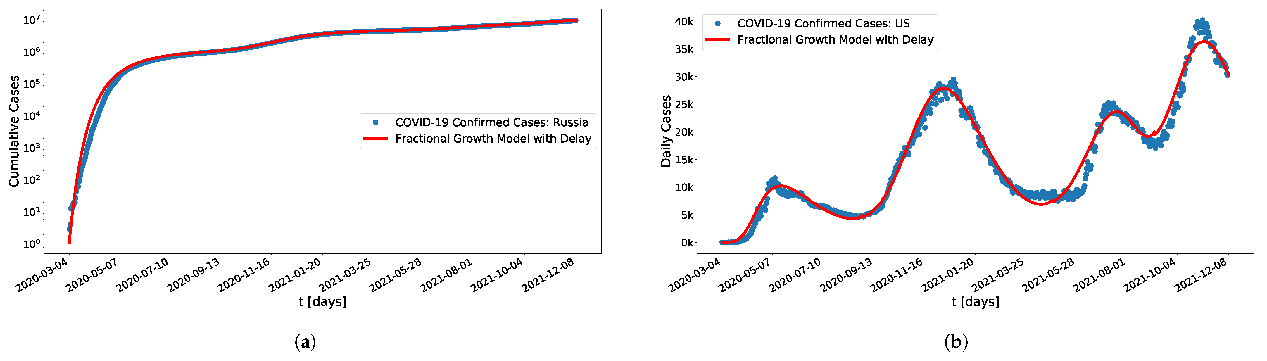
5.2. US Data
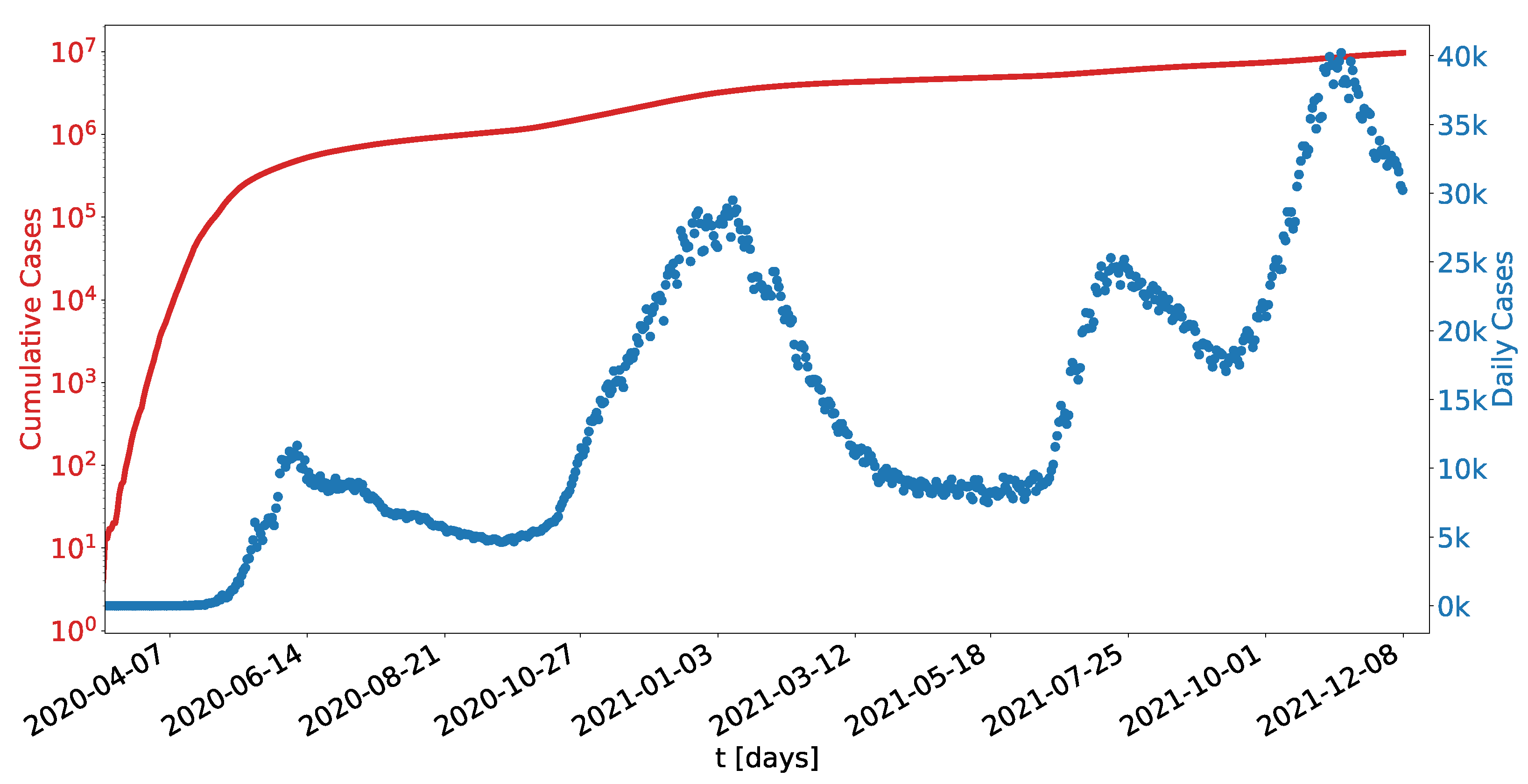
5.3. Russia Data
6. Conclusions
Author Contributions
Funding
Institutional Review Board Statement
Informed Consent Statement
Data Availability Statement
Acknowledgments
Conflicts of Interest
References
- Kuhi, H.D.; Porter, T.; López, S.; Kebreab, E.; Strathe, A.; Dumas, A.; Dijkstra, J.; France, J. A review of mathematical functions for the analysis of growth in poultry. World’s Poult. Sci. J. 2010, 66, 227–240. [Google Scholar] [CrossRef] [Green Version]
- Divya, B.; Kavitha, K. A Review on Mathematical Modelling in Biology and Medicine. Adv. Math. Sci. J. 2020, 9, 5869–5879. [Google Scholar] [CrossRef]
- Asfiji, N.S.; Isfahane, R.D.; Dastjerdi, R.B.; Fakhar, M. Analysis of economic growth differential equations. Soc.-Econ. Debates 2014, 3, 22–30. [Google Scholar]
- Bolton, L.; Cloot, A.H.J.J.; Schoombie, S.W.; Slabbert, J.P. A proposed fractional-order Gompertz model and its application to tumour growth data. Math. Med. Biol. J. IMA 2014, 32, 187–209. [Google Scholar] [CrossRef] [PubMed]
- Xu, H. Analytical approximations for a population growth model with fractional order. Commun. Nonlinear Sci. Numer. Simul. 2009, 14, 1978–1983. [Google Scholar] [CrossRef]
- Malthus, T. An Essay on the Principle of Population (1798); Yale University Press: New Haven, CT, USA, 2013. [Google Scholar]
- Verhulst, P.F. Recherches mathématiques sur la loi d’accroissement de la population. J. ÉConomistes 1845, 12, 276. [Google Scholar]
- XXIV. On the nature of the function expressive of the law of human mortality, and on a new mode of determining the value of life contingencies. In a letter to Francis Baily, Esq. F. R. S. &c. Philos. Trans. R. Soc. Lond. 1825, 115, 513–583. [Google Scholar] [CrossRef]
- Golmankhaneh, A.K.; Cattani, C. Fractal Logistic Equation. Fractal Fract. 2019, 3, 41. [Google Scholar] [CrossRef] [Green Version]
- Krishnaveni, K.; Kannan, K.; Balachandar, S. Approximate analytical solution for fractional population growth model. Int. J. Eng. Technol. 2013, 5, 2832–2836. [Google Scholar]
- Markov, S.M. Reaction networks reveal new links between Gompertz and Verhulst growth functions. Biomath 2019, 8, 1904167. [Google Scholar] [CrossRef] [Green Version]
- Suansook, Y.; Paithoonwattanakij, K. Dynamic of logistic model at fractional order. In Proceedings of the 2009 IEEE International Symposium on Industrial Electronics, Seoul, Korea, 5–8 July 2009. [Google Scholar] [CrossRef]
- Frunzo, L.; Garra, R.; Giusti, A.; Luongo, V. Modeling biological systems with an improved fractional Gompertz law. Commun. Nonlinear Sci. Numer. Simul. 2019, 74, 260–267. [Google Scholar] [CrossRef] [Green Version]
- Wu, G.C.; Baleanu, D. Discrete fractional logistic map and its chaos. Nonlinear Dyn. 2013, 75, 283–287. [Google Scholar] [CrossRef]
- El-Sayed, A.; El-Mesiry, A.; El-Saka, H. On the fractional-order logistic equation. Appl. Math. Lett. 2007, 20, 817–823. [Google Scholar] [CrossRef] [Green Version]
- Tarasov, V.E. Exact Solutions of Bernoulli and Logistic Fractional Differential Equations with Power Law Coefficients. Mathematics 2020, 8, 2231. [Google Scholar] [CrossRef]
- Abdeljawad, T.; Al-Mdallal, Q.M.; Jarad, F. Fractional logistic models in the frame of fractional operators generated by conformable derivatives. Chaos Solitons Fractals 2019, 119, 94–101. [Google Scholar] [CrossRef]
- Piotrowska, M.J.; Foryś, U. The nature of Hopf bifurcation for the Gompertz model with delays. Math. Comput. Model. 2011, 54, 2183–2198. [Google Scholar] [CrossRef]
- Bodnar, M.; Piotrowska, M.J.; Foryś, U. Gompertz model with delays and treatment: Mathematical analysis. Math. Biosci. Eng. 2013, 10, 551. [Google Scholar]
- Bhalekar, S.; Daftardar-Gejji, V. A predictor-corrector scheme for solving nonlinear delay differential Equations of fractional order. J. Fract. Calc. Appl. 2011, 1, 1–9. [Google Scholar]
- Yang, Z.; Cao, J. Initial value problems for arbitrary order fractional differential Equations with delay. Commun. Nonlinear Sci. Numer. Simul. 2013, 18, 2993–3005. [Google Scholar] [CrossRef]
- Hu, J.B.; Lu, G.P.; Zhang, S.B.; Zhao, L.D. Lyapunov stability theorem about fractional system without and with delay. Commun. Nonlinear Sci. Numer. Simul. 2015, 20, 905–913. [Google Scholar] [CrossRef]
- Wang, Z. A Numerical Method for Delayed Fractional-Order Differential Equations. J. Appl. Math. 2013, 2013, 1–7. [Google Scholar] [CrossRef]
- Wang, F.F.; Chen, D.Y.; Zhang, X.G.; Wu, Y. The existence and uniqueness theorem of the solution to a class of nonlinear fractional order system with time delay. Appl. Math. Lett. 2016, 53, 45–51. [Google Scholar] [CrossRef]
- Morgado, M.L.; Ford, N.J.; Lima, P.M. Analysis and numerical methods for fractional differential equations with delay. J. Comput. Appl. Math. 2013, 252, 159–168. [Google Scholar] [CrossRef]
- Čermák, J.; Horníček, J.; Kisela, T. Stability regions for fractional differential systems with a time delay. Commun. Nonlinear Sci. Numer. Simul. 2016, 31, 108–123. [Google Scholar] [CrossRef]
- World Health Organization. Coronavirus Disease (COVID-19) Pandemic. Available online: https://www.who.int/emergencies/diseases/novel-coronavirus-2019/events-as-they-happen (accessed on 8 December 2021).
- COVID-19 Forecasts for Cuba Using Logistic Regression and Gompertz Curves. MEDICC Rev. 2020, 22, 32. [CrossRef]
- Husniah, H.; Supriatna, A.K. Modified Verhulst Logistic Growth Model Applied to COVID-19 Data in Indonesia as One Example of Model Refinement in Teaching Mathematical Modeling. In Proceedings of the 2nd African International Conference on Industrial Engineering and Operations Management, IEOM, Harare, Zimbabwe, 7–10 December 2020. [Google Scholar]
- Torrealba-Rodriguez, O.; Conde-Gutiérrez, R.; Hernández-Javier, A. Modeling and prediction of COVID-19 in Mexico applying mathematical and computational models. Chaos Solitons Fractals 2020, 138, 109946. [Google Scholar] [CrossRef]
- Tuan, N.H.; Mohammadi, H.; Rezapour, S. A mathematical model for COVID-19 transmission by using the Caputo fractional derivative. Chaos Solitons Fractals 2020, 140, 110107. [Google Scholar] [CrossRef]
- Alcántara-López, F.; Fuentes, C.; Chávez, C.; Brambila-Paz, F.; Quevedo, A. Fractional Growth Model Applied to COVID-19 Data. Mathematics 2021, 9, 1915. [Google Scholar] [CrossRef]
- Liu, F.; Huang, S.; Zheng, S.; Wang, H.O. Stability Analysis and Bifurcation Control For a Fractional Order SIR Epidemic Model with Delay. In Proceedings of the 2020 39th Chinese Control Conference (CCC), Shenyang, China, 27–29 July 2020. [Google Scholar] [CrossRef]
- Wang, X.; Wang, Z.; Huang, X.; Li, Y. Dynamic Analysis of a Delayed Fractional-Order SIR Model with Saturated Incidence and Treatment Functions. Int. J. Bifurc. Chaos 2018, 28, 1850180. [Google Scholar] [CrossRef]
- Kumar, P.; Erturk, V.S. The analysis of a time delay fractional COVID-19 model via Caputo type fractional derivative. Math. Methods Appl. Sci. 2020. [Google Scholar] [CrossRef]
- Teodoro, G.S.; Machado, J.T.; De Oliveira, E.C. A review of definitions of fractional derivatives and other operators. J. Comput. Phys. 2019, 388, 195–208. [Google Scholar] [CrossRef]
- Sabatier, J.; Agrawal, O.P.; Machado, J.T. Advances in Fractional Calculus; Springer: Berlin/Heidelberg, Germany, 2007; Volume 4. [Google Scholar]
- Baleanu, D.; Diethelm, K.; Scalas, E.; Trujillo, J.J. Fractional Calculus: Models and Numerical Methods; World Scientific: Singapore, 2012; Volume 3. [Google Scholar]
- Bellen, A.; Zennaro, M. Numerical Methods for Delay Differential Equations; Oxford University Press: Oxford, UK, 2013. [Google Scholar]
- Diethelm, K.; Ford, N.J. Analysis of fractional differential equations. J. Math. Anal. Appl. 2002, 265, 229–248. [Google Scholar] [CrossRef] [Green Version]
- COVID-19 Tablero México-CONACYT-CentroGeo-GeoInt-DataLab. Available online: https://datos.covid-19.conacyt.mx/ (accessed on 8 December 2021).


| Parameters | [days] | [cccc] 1 | [days ] | [cccc] 1 | |||
|---|---|---|---|---|---|---|---|
| Optimal value | 0 | First Sprout | |||||
| Lower bound | 0 | ||||||
| Upper bound | 0 | ||||||
| Optimal value | 215 | Second Sprout | |||||
| Lower bound | 215 | ||||||
| Upper bound | 215 | ||||||
| Optimal value | 440 | Third Sprout | |||||
| Lower bound | 440 | ||||||
| Upper bound | 440 |
| Parameters | [days] | [cccc] 1 | [days ] | [cccc] 1 | |||
|---|---|---|---|---|---|---|---|
| Optimal value | 0 | First Outbreak | |||||
| Lower bound | 0 | ||||||
| Upper bound | 0 | ||||||
| Optimal value | 80 | Second Outbreak | |||||
| Lower bound | 80 | ||||||
| Upper bound | 80 | ||||||
| Optimal value | 200 | Third Outbreak | |||||
| Lower bound | 200 | ||||||
| Upper bound | 200 | ||||||
| Optimal value | 380 | Fourth Outbreak | |||||
| Lower bound | 380 | ||||||
| Upper bound | 380 | ||||||
| Optimal value | 480 | Fifth Outbreak | |||||
| Lower bound | 480 | ||||||
| Upper bound | 480 |
| Parameters | [days] | [cccc] 1 | [days ] | [cccc] 1 | |||
|---|---|---|---|---|---|---|---|
| Optimal value | 0 | First Outbreak | |||||
| Lower bound | 0 | ||||||
| Upper bound | 0 | ||||||
| Optimal value | 180 | Second Outbreak | |||||
| Lower bound | 180 | ||||||
| Upper bound | 180 | ||||||
| Optimal value | 420 | Third Outbreak | |||||
| Lower bound | 420 | ||||||
| Upper bound | 420 | ||||||
| Optimal value | 550 | Fourth Outbreak | |||||
| Lower bound | 550 | ||||||
| Upper bound | 550 |
| Country | Forecast Peak | Real Peak | |
|---|---|---|---|
| Mexico | 19 July 2020, 11 January 2021, and 13 August 2021 | 1 August 2020, 22 January 2021, and 19 August 2021 | |
| US | 13 April 2020, 1 August 2020, 20 December 2020, 10 April 2021, and 31 August 2021 | 7 April 2020, 19 July 2020, 8 January 2021, 11 April 2021, 29 August 2021 | |
| Russia | 17 May 2020, 10 December 2020, 18 July 2021, and 6 November 2021 | 11 May 2020, 24 December 2020, 9 July 2021, and 6 November 2021 |
Publisher’s Note: MDPI stays neutral with regard to jurisdictional claims in published maps and institutional affiliations. |
© 2022 by the authors. Licensee MDPI, Basel, Switzerland. This article is an open access article distributed under the terms and conditions of the Creative Commons Attribution (CC BY) license (https://creativecommons.org/licenses/by/4.0/).
Share and Cite
Alcántara-López, F.; Fuentes, C.; Chávez, C.; López-Estrada, J.; Brambila-Paz, F. Fractional Growth Model with Delay for Recurrent Outbreaks Applied to COVID-19 Data. Mathematics 2022, 10, 825. https://doi.org/10.3390/math10050825
Alcántara-López F, Fuentes C, Chávez C, López-Estrada J, Brambila-Paz F. Fractional Growth Model with Delay for Recurrent Outbreaks Applied to COVID-19 Data. Mathematics. 2022; 10(5):825. https://doi.org/10.3390/math10050825
Chicago/Turabian StyleAlcántara-López, Fernando, Carlos Fuentes, Carlos Chávez, Jesús López-Estrada, and Fernando Brambila-Paz. 2022. "Fractional Growth Model with Delay for Recurrent Outbreaks Applied to COVID-19 Data" Mathematics 10, no. 5: 825. https://doi.org/10.3390/math10050825
APA StyleAlcántara-López, F., Fuentes, C., Chávez, C., López-Estrada, J., & Brambila-Paz, F. (2022). Fractional Growth Model with Delay for Recurrent Outbreaks Applied to COVID-19 Data. Mathematics, 10(5), 825. https://doi.org/10.3390/math10050825