Abstract
Multiphysics or multiscale problems naturally involve coupling at interfaces which are manifolds of lower dimensions. The block-diagonal preconditioning of the related saddle-point systems is among the most efficient approaches for numerically solving large-scale problems in this class. At the operator level, the interface blocks of the preconditioners are fractional Laplacians. At the discrete level, we propose to replace the inverse of the fractional Laplacian with its best uniform rational approximation (BURA). The goal of the paper is to develop a unified framework for analysis of the new class of preconditioned iterative methods. As a final result, we prove that the proposed preconditioners have optimal computational complexity , where N is the number of unknowns (degrees of freedom) of the coupled discrete problem. The main theoretical contribution is the condition number estimates of the BURA-based preconditioners. It is important to note that the obtained estimates are completely analogous for both positive and negative fractional powers. At the end, the analysis of the behavior of the relative condition numbers is aimed at characterizing the practical requirements for minimal BURA orders for the considered Darcy–Stokes and 3D–1D examples of coupled problems.
Keywords:
coupled problems; fractional elliptic equations; preconditioning; BURA method; computational complexity MSC:
35M31; 35R11; 65F08; 65F10; 65N30
1. Introduction
This study is devoted to the development of computationally efficient methods for numerically solving multiphysics and multiscale problems. A representative set of such examples is discussed in the review article [1]. Such applications are also considered in [2,3,4]. More specifically, our attention is focused on a class of problems that involve coupling at interfaces, which are manifolds of lower dimensions. Such mathematical models are often described by saddle-point systems of differential equations. For example, this is the case when either a mixed formulation is used to ensure better accuracy and robustness or when Lagrangian multipliers are introduced to interpret the coupling at the interface. Thus, interface conditions in fractional Sobolev spaces naturally appear. For more related details, we can refer to [5,6,7].
Aimed at presumably more realistic applications, we are interested in the numerical solutions of multidimensional boundary value problems in bounded domain with general geometry . We assume that the geometry of the interface is general, as well. After discretization by a certain mesh method (such as finite differences, finite elements, finite volumes, etc.) on a properly generated unstructured mesh (with possible mesh refinements), we obtain a system of linear algebraic equations with a sparse unstructured matrix . Under the above assumptions, the discrete problems are apparently very large scale. For such problems, the advantages of iterative solution methods (solvers) are well expressed. Note that the condition number of the corresponding matrix can be very large. It could be due not only to the number of degrees of freedom but also to the structure of the mesh. For the multiscale and multiphysical problems under consideration, the media can be very highly heterogeneous and the anisotropy ratio can be very large. Thus, looking for solvers of optimal computational complexity gives rise to the requirement for efficient and robust preconditioning.
The block-diagonal preconditioning is among the most efficient approaches for numerically solving the studied saddle-point problems. Let us consider the system of differential equations written in the block-operator form
where the first rows correspond to the volume equations while the last one represents the interface condition.
Definition 1.
The block-diagonal preconditioners have zero off-diagonal blocks and nonsingular diagonal blocks. They are also known as additive preconditioners.
In this study, we analyze two types of block preconditioners that have optimal convergence rate, that is, the number of iterations is . Following the notation from Equation (1), they can be written as follows:
and
where , respectively . The first blocks of and are selfadjoint positive definite differential operators, is the identity operator at the interface , and stands for the Laplacian at .
At discrete level, the implementation of the first blocks of requires solving systems with sparse symmetric and positive definite (SPD) matrices. The same holds true for the first blocks of . For all of them, a standard PCG (e.g., AMG) solver of optimal computational complexity can be applied. The matrices, corresponding to the last blocks, are dense.
Thus, for the application of the preconditioner , the solution of a system with a matrix in the form is required, while the implementation of leads to matrix vector multiplication with . Here, stands for the matrix corresponding to the discretization of . In both cases, numerical computations with a fractional power in the unit interval of an SPD matrix are involved—either via solving a linear system of equations or via a matrix-vector multiplication. As we will see later on, although the implementation of the last block of is inverse free, it is not less challenging (but even more complicated) than the case of .
In this context, multigrid methods for discrete fractional Sobolev spaces are developed in [5]. The abstract additive multilevel framework is adapted there. The constructed smoother involves small blocks in the form , where is the graph-degree of the mesh node k.
As an alternative, we propose to use the best uniform rational approximation (BURA) method for [8,9,10,11]. The aim is to develop a robust preconditioning algorithm of optimal computational complexity. As correctly noted in [5], a disadvantage of the method introduced in 2018 in [11] was that the accuracy depended on the condition number of the matrix . This drawback has been overcome in the improved BURA approximation developed in [10]; see also the survey paper [8]. It reads as , where is the best uniform rational approximation of degree k of on and is the smallest eigenvalue of . The error of the BURA approximation decreases with k, satisfying the asymptotic estimate . Further improvement of the computational efficiency of the method is presented in [9], where problem-specific model reduction techniques are utilized.
The structure of the paper is as follows. Two examples of coupled multiphysics problems, leading to the class of discussed block-diagonal preconditioners, are presented in Section 2. Section 3 is devoted to the construction and the basic properties of the BURA method. Then, the accuracy of the BURA-based preconditioners is analyzed in Section 4, including the derived estimates for the corresponding condition number. The theoretical results are supported by representative numerical experiments. The implementation issues are discussed in Section 5, ending with the proof of optimal computational complexity of the studied methods and algorithms. The motivation for the choice of numerical tests presented in Section 6 is twofold. On one hand, they illustrate the accuracy of the derived theoretical estimates, while on the other, they provide an additional practical insight for the efficient usage of BURA preconditioners with a small degree k. Finally, we give some conclusions in Section 7.
2. Monolithically Coupled Multiphysics Problems: Two Examples
In this section, we present two examples of related multiphysics problems that lead to block-diagonal preconditioners in the form (2) and (3). These preconditioners are already known and they are important for the analysis, presented in this paper as real world examples, where fractional elliptic problems are formulated. In this paper, we do not analyze the specific properties of the approximations of multiphysics equations or the influence of the different blocks of the preconditioner on the total condition number of the preconditioned system. The main goal of our study is to obtain detailed and asymptotically exact estimates of the accuracy of the BURA method. To simplify notation, throughout the paper we will use N for both the size of an SPD matrix and the number of unknowns of a coupled discrete problem. From the context, it will be clear to which of the two possibilities N refers to. Similarly, we denote by various SPD matrices and again the context will clarify the particular object of interest.
2.1. Example 1: Coupling of Darcy and Stokes Flows
Let be a closed domain in , which is a disjoint union of two subdomains and , that is, . Figure 1 shows two examples of model problems with simple geometry and more realistic problem with a more general geometry of the interface.
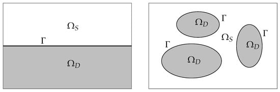
Figure 1.
Darcy–Stokes system in a rectangle domain : model problem with simple geometry (left) and more realistic problem with a more general geometry of the interface (right).
The exchange through the interface between a Stokes flow in and a Darcy flow in is modeled by the system of equations in the form [7,12,13]:
Here, , are the velocities and pressure for the Stokes problem in , , are the velocities and pressure for the Darcy problem in , K and are the hydraulic conductivity, respectively, the fluid viscosity, while the coefficient D corresponds to the Beavers–Joseph–Saffman condition. Finally, and are unit vectors that are normal and tangential to the interface . We further assume that the problem is equipped with correct boundary conditions.
Similarly to (1), the system of differential Equation (4) can be written in the block-operator form , where
The block sparsity structure is shown here. Then, after discretization by some mesh method (such as finite elements, finite differences, or finite volumes) we will obtain a linear system, where all blocks that correspond to nonzero operators in (5) will be also sparse.
There are two groups of methods for preconditioned iterative solution of coupled multiphysics problems: monolithic and based on some splitting [5,14,15]. For example, splitting techniques include operational splitting (by physical processes), domain decomposition (geometrical splitting), and block partitioning (algebraic splitting). The methods considered in this paper belong to the second group, following the motivation from [13]. Additionally, our study is supported by some recent achievements in the solution methods for fractional diffusion problems, or more generally for linear algebraic systems with fractional power of sparse SPD matrices.
The case is considered in [13]. It should be noted that this simplified problem is representative enough to illustrate why the norms studied in [12] are not sufficient for the proposed preconditioning approach. In [16], it is shown that the block-diagonal preconditioner
provides an optimal condition number estimate. Here, is a tangential trace operator, while stands for the identity operator. The first four blocks of (6) are standard components for preconditioning Darcy and Stokes problems. Thus, after discretization, the matrices corresponding to the first two blocks are sparse SPD, to which some Preconditioned Conjugate Gradients (PCG) solver (e.g., AMG) of optimal computational complexity can be applied. Note that the local operator only increases the diagonal dominance in the first block. The last block leads to a system with the dense matrix .
This example raises the question of the efficient solution/preconditioning of systems with matrices in the form , is sparse SPD, . Until recently, this was a challenge.
2.2. Example 2: Coupling a 1D Structure Embedded in
Let be a bounded domain, while represents a 1D manifold (structure) inside , see Figure 2. The following trace coupled problem is considered [17]:
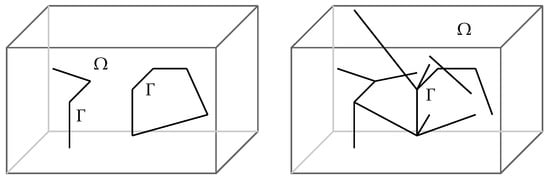
Figure 2.
Coupled 3D–1D systems in a hexahedral domain : model problems with single line geometry of the interfaces (left) and more realistic problem with more general geometry of the interface (right).
Here u, v, p are unknowns, the 1D manifold is parameterized in terms of s, the Laplacian on is understood in terms of the Laplace–Beltrami operator, is a suitable trace operator, and is a Dirac measure such that for a continuous function w.
At the same time, it is worth noting that the equations used in the real-life simulations are more complicated than (7); thus, the above example can be considered as a relevant model problem.
As it can be seen in [17], the standard finite element methods provide accurate error estimates in the norms of the introduced fractional order Sobolev spaces. The saddle-point matrix corresponding to the obtained system of linear algebraic equations is sparse. Arguments, similar to those discussed after (4) in the case of the Darcy–Stokes problem, are applicable here. However, standard techniques are not directly applicable to effective preconditioning. In what follows, we will consider the block-diagonal preconditioner
introduced in [6]. The choice of the fractional power in the third block of (8) is analyzed there, observing that values yield bounded condition numbers. The presented additional stability analysis has led to the preferred value . Similar arguments to those concerning the implementation of the preconditioner are applicable to .
The efficient approximate matrix vector multiplication with the matrix , where is a sparse SPD matrix and , is the challenging question raised by this example.
2.3. Implementation of and : The Key Question
The key questions in implementing the block-diagonal preconditioners and are raised by the last blocks. They concern the fractional powers of SPD matrices defined through the spectral decomposition
where the columns of are the orthonormal eigenvectors of and stands for the diagonal matrix of the related eigenvalues. Under these assumptions, , the matrix is unitary, , which leads directly to (9). Therefore
The Formula (10) could be used in practical computations if the N eigenvectors and eigenvalues are explicitly known and if the matrix vector multiplication with is equivalent to a fast Fourier transform. In such cases, the computational complexity is almost linear, . However, when talking about fractional Laplacian on , this limits the applications to interfaces with simple geometry (like the left sides of Figure 1 and Figure 2), uniform meshes, and to the lowest order finite element approximations.
The multigrid methods proposed and analyzed in [5] are aimed at handling general geometries of the interface . As noted in the Introduction, the smoother includes non-local (dense) but small blocks , where is the graph-degree of the mesh node k. Under certain regularity assumptions and fixed number of the multigrid levels J, the condition number is uniformly bounded for each given . More precisely, or , depending on the regularity assumptions.
The case of negative power corresponds to the preconditioner (3), and more specifically to (8). The implementation of this kind of preconditioner requires a matrix vector multiplication with . For this multiplication, one can use the representation
thus reducing the problem to numerically solving linear system with , . Following (11), the second variant of the multigrid method in [5] is adapted to handle negative powers. The condition number of the proposed preconditioner depends on N, including the case of a fixed number of multigrid levels J.
In the following sections, we consider the application of the BURA method in the general framework of the preconditioners and (Equations (2) and (3)) and, respectively, and (Equations (6) and (8)). Our study is aimed at developing uniformly bounded condition number estimates, which are robust in terms of the geometry of the interface, as well as in terms of regularity of the solution. The ultimate goal is to obtain preconditioned solution methods of optimal computational complexity.
3. The BURA Method
The fractional diffusion problems are non-local and their numerical solution is costly. The survey paper [8] tracks some of the last years’ achievements on this topic. They include a variety of methods based on: (i) extension of the problem from to a local elliptic problem in , (ii) reformulation as a pseudo-parabolic problem in the cylinder , (iii) methods based on approximation of the Dunford–Taylor integral representation of the solution, and (iv) methods based on the best uniform rational approximation (BURA) of on . Applying rational approximations is one of the most successful approaches to efficiently solve non-local problems. For example, following the reformulation to a pseudo-parabolic problem, an efficient method based on diagonal Padé approximation to is developed in [18]. Recently, a unified view to the methods based on the approaches (i–iv) was presented in [19], showing that all of them can be interpreted as generated by some rational approximation of on . In this sense, BURA methods are asymptotically the best.
The BURA method is originally introduced in [11] where the solution of the linear algebraic system
is written in the form with , with s a (presumably small) positive integer. The proposed approximate solution method is based on the best uniform rational approximation (BURA) of the function for . Quite promising numerical results for , accompanied by representative comparison analysis with other known methods, were presented in [11]. However, the convergence rate of the first BURA method was not robust with respect to the condition number of , which is correctly noted in [5]. This shortcoming is completely overcome in [10]. Several aspects of the step-by-step development of the BURA method can be traced in the survey paper [8]. Note that in [19], it was shown that the available numerical solvers of (12) are based on uniform rational approximation of , . Therefore, methods based on best uniform rational approximation are expected to be the most efficient. From now on, when we talk about BURA, we will have in mind the following variant of the method proposed and analyzed in [10].
Let be the best uniform rational approximation of in in the class of rational functions , and are polynomials of degree k. The case of rational approximations with equal degrees of the polynomials P and Q is known as the diagonal sequence of the Walsh table. The minimizer satisfies the following sharp exponential error estimate with respect to the degree k [20]:
Then, the BURA approximation of is defined as
where is the smallest eigenvalue of the SPD matrix .
The Padé approximation is also defined in the class of rational functions. However, while the minimizer is implicitly defined, the Padé approximation is a Hermite interpolation. The advantage of the Padé approximation is that it is easier to compute.
Let be obtained after finite difference discretization of a given elliptic operator. In the context of this paper, we can assume that corresponds to the Laplacian with homogeneous Dirichlet boundary conditions. Then, , which follows, e.g., from the Poincaré–Steklov inequality. The same is true if the finite element method (FEM) is applied to discretize the Laplacian. In this case, where and are the stiffens and mass matrices, respectively. Then, the SPD property of the FEM matrix is understood in terms of the inner product induced by the mass matrix .
Let us denote by
the BURA approximation of the solution of the fractional diffusion linear system (12). Then, applying spectral basis representation of , and of , and the Parseval’s formula, we obtain the error estimate (see, for more details [10])
The estimate (14) clearly shows the exponential rate with respect to the degree k of the rational approximation. Moreover, its dependence on the fractional power is explicit. Smaller means lower accuracy. Since is uniformly bounded from below, the estimate is robust with respect to the condition number . The estimate (14) is very sharp. The numerical tests conducted in [9] illustrate how close the computed errors are to the theoretical estimate, when the latter is greater than the double-precision accuracy.
The properties of the single roots and the related interlacing poles of are well studied [21]. Both the additive and the multiplicative representation of the rational function can be used in the implementation of the BURA method. The corresponding matrix valued expressions read as
and
where and . A numerically stable approach for the computation of these coefficients is developed in [22]. Both the additive (15) and the multiplicative (16) algorithms reduce the problem to solving k systems with sparse SPD matrices , which are positive diagonal perturbations of . This leads to the understanding of the degree k as a universal measure for algorithmic efficiency, thus giving rise to the following asymptotic estimate of computational efficiency of the BURA methods
The estimate (17) holds true if a method with optimal computational complexity is used to solve the auxiliary linear systems that appear in (15) or (16). In the multidimensional case, this means that such a preconditioned iterative solver is applied. In the numerical tests presented in our previous papers [9,11,23], the Boomer-AMG implementation from HYPRE [14] of the algebraic multigrid (AMG) preconditioner in the PCG framework is used for this purpose.
The computational complexity depends on the target accuracy of the numerical solution. Assume that the matrix corresponds to FEM discretization of the fractional diffusion problem. The rigorous error analysis is a task beyond the standard theory of FEM. Such error bounds are derived in [24] under certain assumptions that are an interplay among data regularity, regularity pickup of the differential operator (e.g., the Laplacian), and the fractional power . If linear finite elements are used and if , the error is essentially
The case where the finite difference method (FDM) is applied for discretization of the fractional diffusion problem is analyzed in [10]. The presented error estimates are based on certain equivalence between the lumped mass FEM approximation and the -stencil FDM approximation.
The further analysis integrates the FEM/FDM error estimate (18) in the complexity estimate (17). Assuming the mesh is quasi uniform, , with , and therefore
Then, for a given mesh parameter h, the degree of BURA approximation k is chosen such that the contributions of the discretization error (18) and the BURA error (14) to the total error are balanced. In this way, and taking into account (17), the following almost optimal computational complexity
is derived in [10].
More recently, the so-called reduced additive BURA-AR and multiplicative BURA-MR methods were introduced in [9]. This study follows the observation that the matrices of part of the auxiliary systems possess very different properties. An important observation is that under certain assumptions, the computational complexity of the reduced BURA can be improved to .
4. Bura Preconditioning: Condition Number Estimates
The iterative solution of fractional diffusion problems can be applied in very limited cases. Note that even if a good preconditioner is available, the matrix vector multiplication with remains an open problem in the general case.
The study in this paper is motivated by the application of the BURA approximation of in the spirit of block-diagonal preconditioners (6), (8) of the coupled problems (4), (7), respectively. In these specific cases, the preconditioned iterative solvers are applied to sparse matrices, and therefore the matrix vector multiplication does not create computational difficulties.
Consider the matrix , . Here, we assume the is a sparse SPD matrix obtained after FDM or FEM discretization of a given elliptical (say Laplacian) boundary value problem with a mesh parameter h. Denote by the spectrum of , where are the monotonically increasing positive eigenvalues and are the corresponding normalized eigenvectors. Then
4.1. Bura Preconditioner :
Following the BURA approximation of , we introduce the preconditioner of by its inverse
Lemma 1.
Assume that the degree k is large enough so that . Then, the following condition number estimate for the BURA preconditioner , , holds true
4.2. Bura Preconditioner :
In this case, . Thus, we consider the preconditioner in the form
Lemma 2.
Assume that the degree k is large enough so that . Then, the following condition number estimate for the BURA preconditioner , , holds true
Proof.
According to (19), the spectrum of the new preconditioner is as follows
Following the notations and arguments from the proof of Lemma 1, we obtain
Hence
and the proof is completed.
5. Preconditioning of the Coupled Problems: Condition Number Estimates and Computational Complexity
Let us assume that proper FDM or FEM is applied for numerical solution of the coupled problems (4) and (7). Thus, we obtain the block-diagonal preconditioner
corresponding to (6) and
corresponding to (8). As in the continuous case, the preconditioners and provide optimal condition number estimates of the saddle-point matrices corresponding to (4) and (7).
Now, the block-diagonal preconditioners and are introduced by replacing the last (interface) blocks in (26) and (27) by their rational approximations, as defined in the previous section. In this way, we obtain
where is determined following (20), and
with defined through (23).
The following assumptions will be used in the analysis of the introduced BURA preconditioners:
- (A1)
- Quasi uniform meshes with mesh parameter h are used for FDM/FEM approximation of the considered coupled problems. Thus, the number of unknowns for the discrete Darcy–Stokes problem is , and similarly, for the 1D–3D coupling problem, . In both cases, the number of unknowns related to the interface is .
- (A2)
- Solvers of optimal computational complexity are applied for the systems with sparse SPD matrices which appear in the implementation of the BURA preconditioners.
5.1. Preconditioner
Lemma 3.
Let the assumptions A1 and A2 be fulfilled, and let k be the minimal degree of the rational approximation of the last block in (28) such that
where is an a priori chosen constant. Then,
Proof.
The difference between block-diagonal preconditioners and is in last blocks only. Consequently, the estimate (30) follows directly from Lemma 1. □
For example, following the estimate from Lemma 3, and choosing , we obtain the bound . Obviously, this condition number can be arbitrary close to 1 if is small enough. However, this might be computationally expensive, taking into account that smaller gives rise to larger degree k of the applied BURA approximation.
The block-diagonal preconditioner has an optimal convergence rate, provided the assumptions of Lemma 3 are met. This means that iterations are sufficient to solve the discrete Darcy–Stokes problem. Therefore, the question is what the computational complexity of solving a system with is. It can be written in the form
where is the complexity of solving a system with the i-th diagonal block. It follows from the assumptions (A1) and (A2) that
and
Let us recall that . Thus, the assumptions of Lemma 3 are valid if and only if , and therefore
The presented analysis is summarized in the following theorem.
Theorem 1.
Under the assumptions of Lemma 3, the preconditioned iterative solution of a discrete Darcy–Stokes problem with the preconditioner has an optimal computational complexity.
Proof.
The statement follows directly from the above estimates of , , and their sum, that is
□
5.2. Preconditioner
Lemma 4.
Let the assumptions A1 and A2 be fulfilled. We also assume that k is the minimal degree of the rational approximation such that
where is a chosen constant. Then,
Proof.
Again, the difference between the block-diagonal preconditioners and is in the interface blocks only, and the proof is analogous to the one of Lemma 3. □
The block-diagonal preconditioner has an optimal convergence rate if the assumptions of Lemma 4 are met. This raises the important question about the computational complexity of solving a system with . In this case, we write it in the form
It follows from the assumptions (A1) and (A2) that
and
Then, the analogue of Theorem 1 reads as follows.
Theorem 2.
Under the assumptions of Lemma 4, the preconditioned iterative solution of a discrete 3D–1D coupled problem with the preconditioner has an optimal computational complexity.
Proof.
The result follows directly from the estimates of , , and their sum as follows
□
Theorems 1 and 2 show the asymptotic optimality of the proposed BURA preconditioners. The efficient implementation of the corresponding iterative solution methods depends on the condition number estimates given by Lemmas 3 and 4. They are controlled by the constants and . Some practical aspects related to the balance of these parameters are presented in the next section.
For large discrete linear systems approximating discrete fractional elliptic equations, parallel multigrid solvers are used. The efficiency of these solvers is studied in [25] and the references therein. We refer to recommendations given in this paper.
6. Behavior of the Condition Numbers of the BURA-Based Preconditioners
In this section, we will numerically analyze the behavior of the estimates for the condition numbers of the BURA-based preconditioners. The theoretical estimates derived in Lemmas 1 and 2 will be compared with those that follow from the definitions of the corresponding rational approximations.
6.1. Analysis of
From the definition (20) of the preconditioner for , we obtain the estimate
where and . The results of the performed tests are presented in Figure 3.
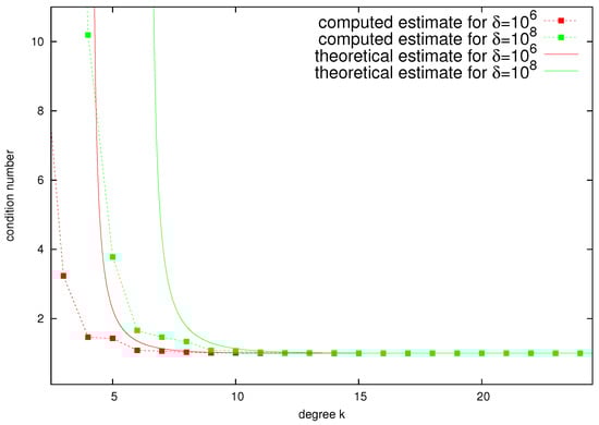
The data obtained via (32) are denoted as computed estimates, while the theoretical estimates are obtained by applying the upper bound (21) from Lemma 1. For the computed estimates, the BRASIL software [26] has been used. The figure includes theoretical estimates for large enough k for which the condition (29) from Lemma 3 is satisfied.
The first observation is that the computed and theoretical estimates are practically the same, being almost equal to one for and all considered cases. Of course, it is not necessary to have a relative condition number that is so close to one. Thus, for , we obtain approximately that when . For , the same holds true when .
The relative condition number depends on . However, the presented results can be assessed as very promising. Assume that for the problem under consideration in , a quasi-uniform triangulation with mesh parameter h is used. Then, the size of the discrete problem is . Thus, means , which is more or less the largest size of the most commonly solved 2D problems. In this sense, the tests in Figure 3 are fully representative.
6.2. Analysis of
Here, we adopt the approach, assumptions, and notations form the previous subsection. Now, from the definition (23) of the preconditioner for , we obtain the estimate
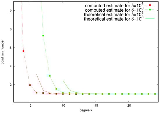
In this figure, the data for the theoretical estimates start from the first k for which the condition (31) in Lemma 4 is satisfied. Similar to Figure 3, the relative condition number is close to one if for both values of . Here, for , we see that when . For , the same holds true when .
Assume now that for the problem of coupling a 1D structure embedded in , a quasi-uniform mesh with a parameter h is used. Then, the size of the discrete problem is and therefore means . Such extremely large-scale 3D problems are a challenge for even the most powerful supercomputers today. Thus, can be considered as a limit case when analyzing the preconditioner .
6.3. Comparative Summary
The preconditioned interface problems discussed in the previous two sections are significantly different, due to the alternating sign of the degrees and . However, the condition number estimates for the proposed BURA preconditioners are very similar. Thus, the definition (23) implies the equality
therefore the analysis can be reduced to the case of positive fractional powers. From this point of view, the estimates (21) from Lemma 1 and (24) from Lemma 2 show certain advantages of compared to . This follows from the better exponential accuracy of the BURA method for larger . However, this conclusion is asymptotically true, that is, for large enough k. The data in Figure 3 and Figure 4 show a different picture. This is the motivation to present more detailed information about the behavior of and for in Table 1.

Table 1.
Computed estimates of and with respect to , for .
The presented data confirm the promising assessment of the BURA preconditioners. We observe a stable behavior of the computed estimates of the condition numbers. If needed, the tabular results can be used for good enough piecewise linear interpolation for arbitrary .
As noted in the Introduction, our study is partly motivated by the multigrid methods for discrete fractional Sobolev spaces presented in [5]. For the 1D fractional Laplacian in the interval and uniform mesh, the reported relative condition number of the multigrid preconditioner for and for the maximal size is . The spectrum of for this model problem is known. Thus, to compare with the data from Table 1, we recall that corresponds to . In the case of negative fractional power, we interpolate the presented tabular data to obtain the corresponding relative condition number . These simple examples illustrate the competitiveness of the BURA preconditioners. The potential benefits of the new method will be even greater for coupled problems with more complex geometry .
7. Concluding Remarks
The fractional diffusion operators are non-local, and the related matrices are dense. Furthermore, when using the spectral definition, the matrix is generally non-computable. In such a situation, we are not even able to compute the residual, which should directly rule out the idea of applying any iterative solution methods to systems in the form .
Why, then, do we discuss preconditioning methods for ? For the considered coupled problems such preconditioning makes sense, as the corresponding systems have sparse matrices (so computing of the residue is not a problem), while the fractional power matrices appear only in the block-diagonal preconditioners (6) and (8).
Our study is motivated by the results of the recently published papers [5,13,17], where the developed multigrid methods for discrete fractional Sobolev spaces are applied to the Darcy–Stokes and 3D–1D coupled problems. Alternatively, we have proposed a fully algebraic preconditioning approach.
For , the new preconditioner relies directly on the best uniform rational approximation (BURA) of degree k of . An important further contribution is the construction of for leading to the equality
This allowed us to develop a unified approach to the relative condition number estimates (21) and (24), applied later in Theorem 1 and Theorem 2, where the optimal computational complexity for both considered coupled problems is proved. The numerical study of and is also important for the value of the paper. As shown, a very small degree of k is practically sufficient to ensure high quality BURA preconditioning.
In general, it is clear that a required accuracy can be obtained by applying different known methods for spectral fractional diffusion problems. Here, we apply the BURA method, motivated by its advantages, as proven in [19] (see the discussion at the beginning of Section 3).
For the simplest case of , the comparison with the multigrid preconditioners from [5] illustrates the competitiveness of the newly proposed and . For most of the BURA preconditioners, even stronger numerical advantages can be expected when more complex coupled problems are considered, due to the more general scope of applicability of the presented results. Among the other advantages, we note the following: BURA preconditioners are purely algebraic, so regularity assumptions are not made in the theoretical analysis. The theoretical estimates (21) and (24), as well as those shown in Table 1, are exactly the same for every type of geometry of . The BURA approach and the obtained condition number estimates are applicable to a wider class of problems, including, for example, coupling of a 2D manifold embedded in .
Author Contributions
Conceptualization, S.M.; Formal analysis, I.L.; Funding acquisition, S.H. and S.M.; Methodology, S.H. and S.M.; Project administration, S.M.; Software, I.L.; Visualization, I.L.; Writing—original draft, S.M.; Writing—review & editing, S.H. and I.L. All authors have read and agreed to the published version of the manuscript.
Funding
This research was funded by Grant No. BG05M2OP001-1.001-0003, financed by the Science and Education for Smart Growth Operational Program (2014–2020) and co-financed by the European Union through the European Structural and Investment and by the Bulgarian National Science Fund under grant No. DFNI-DN12/1.
Institutional Review Board Statement
Not applicable.
Informed Consent Statement
Not applicable.
Data Availability Statement
Not applicable.
Acknowledgments
We acknowledge the provided access to the e-infrastructure and support of the Centre for Advanced Computing and Data Processing, with the financial support by the Grant No. BG05M2OP001-1.001-0003, financed by the Science and Education for Smart Growth Operational Program (2014–2020) and co-financed by the European Union through the European Structural and Investment funds. The work is partially supported by the Bulgarian National Science Fund under grant No. DFNI-DN12/1.
Conflicts of Interest
The authors declare no conflict of interest.
References
- Keyes, D.; McInnes, L.; Woodward, C.; Gropp, W.; Myra, E.; Pernice, M.; Bell, J.; Brown, J.; Clo, A.; Connors, J.; et al. Multiphysics simulations: Challenges and opportunities. Int. J. High Perform. Comput. Appl. 2013, 27, 4–83. [Google Scholar] [CrossRef] [Green Version]
- Mehdizadeh Khalsaraei, M.; Shokri, A.; Molayi, M. The new high approximation of stiff systems of first order IVPs arising from chemical reactions by k-step L-stable hybrid methods. Iran. J. Math. Chem. 2019, 10, 181–193. [Google Scholar]
- Nordsletten, D.; Niederer, S.; Nash, M.; Hunter, P.; Smith, N. Coupling multi-physics models to cardiac mechanics. Prog. Biophys. Mol. Biol. 2011, 104, 77–88. [Google Scholar] [CrossRef]
- Shokri, A.; Mehdizadeh Khalsaraei, M.; Atashyar, A. A new two-step hybrid singularly P-stable method for the numerical solution of second-order IVPs with oscillating solutions. Iran. J. Math. Chem. 2020, 11, 113–132. [Google Scholar]
- Bærland, T.; Kuchta, M.; Mardal, K.A. Multigrid methods for discrete fractional Sobolev spaces. Siam J. Sci. Comput. 2019, 41, A948–A972. [Google Scholar] [CrossRef]
- Kuchta, M.; Mardal, K.A.; Mortensen, M. Preconditioning trace coupled 3D-1D systems using fractional Laplacian. Numer. Methods Partial. Differ. Equ. 2019, 35, 375–393. [Google Scholar] [CrossRef] [Green Version]
- Layton, W.J.; Schieweck, F.; Yotov, I. Coupling fluid flow with porous media flow. Siam J. Numer. Anal. 2002, 40, 2195–2218. [Google Scholar] [CrossRef]
- Harizanov, S.; Lazarov, R.; Margenov, S. A survey on numerical methods for spectral Space-Fractional diffusion problems. Fract. Calc. Appl. Anal. 2020, 23, 1605–1646. [Google Scholar] [CrossRef]
- Harizanov, S.; Kosturski, N.; Lirkov, I.; Margenov, S.; Vutov, Y. Reduced Multiplicative (BURA-MR) and Additive (BURA-AR) Best Uniform Rational Approximation Methods and Algorithms for Fractional Elliptic Equations. Fractal Fract. 2021, 5, 61. [Google Scholar] [CrossRef]
- Harizanov, S.; Lazarov, R.; Margenov, S.; Marinov, P.; Pasciak, J. Analysis of numerical methods for spectral fractional elliptic equations based on the best uniform rational approximation. J. Comput. Phys. 2020, 408, 109285. [Google Scholar] [CrossRef] [Green Version]
- Harizanov, S.; Lazarov, R.; Margenov, S.; Marinov, P.; Vutov, Y. Optimal solvers for linear systems with fractional powers of sparse SPD matrices. Numer. Linear Algebra Appl. 2018, 25, e2167. [Google Scholar] [CrossRef]
- Galvis, J.; Sarkis, M. Non-matching mortar discretization analysis for the coupling Stokes-Darcy equations. Electron. Trans. Numer. Anal 2007, 26, 350–384. [Google Scholar]
- Holter, K.E.; Kuchta, M.; Mardal, K.A. Robust preconditioning for coupled Stokes–Darcy problems with the Darcy problem in primal form. Comput. Math. Appl. 2021, 91, 53–66. [Google Scholar] [CrossRef]
- Falgout, R.D.; Yang, U.M. hypre: A Library of High Performance Preconditioners. In Computational Science—ICCS 2002; Sloot, P.M.A., Hoekstra, A.G., Tan, C.J.K., Dongarra, J.J., Eds.; Lecture Notes in Computer Science; Springer: Berlin/Heidelberg, Germany, 2002; Volume 2331, pp. 632–641. [Google Scholar]
- Zhang, H.; Guo, J.; Lu, J.; Li, F.; Xu, Y.; Downar, T. An assessment of coupling algorithms in HTR simulator TINTE. Nucl. Sci. Eng. 2018, 190, 287–309. [Google Scholar] [CrossRef]
- Holter, K.E.; Kuchta, M.; Mardal, K.A. Robust Preconditioning of Monolithically Coupled Multiphysics Problems. 2020. Available online: https://arxiv.org/abs/2001.05527 (accessed on 28 February 2020).
- Kuchta, M.; Laurino, F.; Mardal, K.A.; Zunino, P. Analysis and approximation of mixed-dimensional PDEs on 3D-1D domains coupled with Lagrange multipliers. Siam J. Numer. Anal. 2021, 59, 558–582. [Google Scholar] [CrossRef]
- Duan, B.; Lazarov, R.; Pasciak, J. Numerical approximation of fractional powers of elliptic operators. IMA J. Numer. Anal. 2020, 40, 1746–1771. [Google Scholar] [CrossRef] [Green Version]
- Hofreither, C. A Unified View of Some Numerical Methods for Fractional Diffusion. Comput. Math. Appl. 2020, 80, 332–350. [Google Scholar] [CrossRef]
- Stahl, H. Best uniform rational approximation of xα on [0, 1]. Bull. Am. Math. Soc. 1993, 28, 116–122. [Google Scholar] [CrossRef] [Green Version]
- Saff, E.B.; Stahl, H. Asymptotic distribution of poles and zeros of best rational approximants to xα on [0, 1]. In Topics in Complex Analysis; Banach Center Publications; Institute of Mathematics, Polish Academy of Sciences: Warsaw, Poland, 1995; Volume 31. [Google Scholar]
- Hofreither, C. An algorithm for best rational approximation based on barycentric rational interpolation. Numer. Algorithms 2021, 88, 365–388. [Google Scholar] [CrossRef]
- Harizanov, S.; Kosturski, N.; Margenov, S.; Vutov, Y. Neumann fractional diffusion problems: BURA solution methods and algorithms. Math. Comput. Simul. 2021, 189, 85–98. [Google Scholar] [CrossRef]
- Bonito, A.; Pasciak, J. Numerical approximation of fractional powers of elliptic operators. Math. Comput. 2015, 84, 2083–2110. [Google Scholar] [CrossRef] [Green Version]
- Čiegis, R.; Starikovičius, V.; Margenov, S.; Kriauzienė, R. Scalability analysis of different parallel solvers for 3D fractional power diffusion problems. Concurr. Comput. Pract. Exp. 2019, 31, e5163. [Google Scholar] [CrossRef]
- Software BRASIL. Available online: https://baryrat.readthedocs.io/en/latest/#baryrat.brasil (accessed on 28 February 2020).
Publisher’s Note: MDPI stays neutral with regard to jurisdictional claims in published maps and institutional affiliations. |
© 2022 by the authors. Licensee MDPI, Basel, Switzerland. This article is an open access article distributed under the terms and conditions of the Creative Commons Attribution (CC BY) license (https://creativecommons.org/licenses/by/4.0/).