Evaluation and Mathematical Analysis of a Four-Dimensional Lotka–Volterra-like Equation Designed to Describe the Batch Nisin Production System

Abstract

Nisin, an antibacterial compound produced by Lactococcus lactis strains, has been approved by the US Food and Drug Administration to be used as a safe food additive to control the growth of undesirable pathogenic bacteria. Nisin is commonly described as a pH-dependent primary metabolite since its production depends on growth and culture pH evolution. However, the relationships between bacteriocin synthesis (BT), biomass production (X), culture pH, and the consumption of the limiting nutrient (total nitrogen: TN) have not been described until now. Therefore, this study aims to develop a competitive four-dimensional Lotka–Volterra-like Equation (predator-prey system) to describe these complex relationships in three series of batch fermentations with L. lactis CECT 539 in diluted whey (DW)-based media. The developed four-dimensional predator-prey system accurately described each individual culture, providing a good description of the relationships between pH, TN, X, and BT, higher values for R² and F-ratios, lower values (<10%) for the mean relative percentage deviation modulus, with bias and accuracy factor values approximately equal to one. The mathematical analysis of the developed equation showed the existence of one asymptotically stable equilibrium point, and the phase’s diagram obtained did not show the closed elliptic trajectories observed in biological predator-prey systems.

1. Introduction

Nisin, a bacteriocin produced by Lactococcus lactis strains, has a wide antibacterial activity against food spoilage and pathogenic bacteria. For this reason, this biomolecule has been recognized by the US Food and Drug Administration as a natural and safe biopreservative in food products, being allowed in the USA and several European Union countries. The advantages of using nisin in foods include the reduction in both the thermal treatment and addition of chemicals to food products and an increase in their shelf life [1].

For high nisin production at low cost, it is necessary to know the relationship between the main culture variables, which could be elucidated with the use of appropriate mathematical models. This could also allow proper monitoring and control of these bioprocesses [2].

Different mathematical models have been commonly used to describe the kinetics of growth (e.g., Verhulst, Gompertz, Richards, Bertalanffy, Weibull, and Monod) and bacteriocin synthesis (e.g., unmodified and modified forms of the Luedeking–Piret model) by lactic acid bacteria (LAB) in batch fermentations [2,3,4,5,6,7,8]. However, these models do not always provide an accurate or reasonable description of the bacteriocin production system.

An appropriate model for biomass production should consider the main factors affecting growth, including the effect of the time-dependent dynamics of other culture variables (culture pH and the concentrations of nutrients and products) [2,3,5,9,10]. In addition, a model describing nisin synthesis should relate the kinetics of product formation rate to the growth rate and biomass concentration [11], but if another factor (e.g., pH or an essential nutrient) produces a specific effect on product synthesis, a term for explaining such an effect should be included in the model [5,9,12]. To the best of our knowledge, there are no models describing the complex relationships between the dynamics of culture pH (pH(t)), the limiting nutrient consumption and production of biomass (X(t)), and bacteriocin (BT(t)) [5,9,11,12].

The three-dimensional Lotka–Volterra (LV) equations were designed for appropriately describing the interactions between three species (two preys-one predator or one prey-two predators) in biological systems [13]. Based on this fact, this three-dimensional LV-like equation was modified to explain, for the first time and in the simplest way, the relationships between the variables pH(t), X(t), and BT(t) in batch cultures of different LAB in various culture media [8]. Nevertheless, the modified three-dimensional equation neither accounts for the effect of total nitrogen (TN(t)) consumption (the growth limiting nutrient in these fermentations [5,8]) on the growth and nisin production, nor includes an equation to describe the dynamics of total nitrogen consumption for biomass and nisin synthesis. This was mainly due to some researchers not quantifying the evolution of TN(t) in the cultures [14].

For this reason, in this study, a four-dimensional equation based on competitive predator-prey system assumptions [15] was developed for the first time, considering the interactions between the main culture variables (pH(t), TN(t), X(t), and BT(t)) implicated in nisin production. Then, we investigated the effectiveness of the designed model for describing the microbiological bacteriocin production system of L. lactis CECT 539 in different batch fermentations in diluted whey (DW) media containing different initial nutrient compositions [16,17,18]. With this approach, an improved description of the complex relationships between the four variables was given.

The values of the biokinetic parameters for each equation were determined by the numerical integration of the four differential equations of the developed model, and their statistical significance was corroborated by using an appropriate statistical analysis. The adequacy and utility of the designed four-dimensional equation were discussed by taking into account the statistical significance of the model parameters, the trends observed in the experimental data, and the different culture media used. Furthermore, the mathematical analysis of the four-dimensional Lotka–Volterra-like equation was also performed by studying its approximated solutions, trajectories, and steady states.

2. Results and Discussion

2.1. Design of the Four-Dimensional Equation

The microbiological four-dimensional Equation (Equations (1)–(4)) was developed considering the following assumptions:

(i)

The culture pH (pH(t)) decline could be described as the difference between the buffer capacity of the medium [19] and the decrease in pH due to lactic acid production by the biomass as follows:

$$\frac{dpH\left(t\right)}{dt}=-pH\left(t\right)·\left(a - b·pH\left(t\right) - c·X\left(t\right)\right)$$

(1)

(ii)

The total nitrogen (TN(t)), the limiting nutrient in these cultures [5], which is channeled into the cells and nisin molecules, could be considered as a prey that is consumed for both biomass and nisin production, and its consumption depends on the culture pH [5,20], as follows:

$$\frac{dTN\left(t\right)}{dt}=-TN\left(t\right)·\left(d - e·TN\left(t\right) - f·X\left(t\right) - g·BT\left(t\right) - h·pH\left(t\right)\right)$$

(2)

(iii)

Biomass (X(t)) could be considered as one predator that grows logistically competing with nisin for the nitrogen source and depending on the culture pH and the TN source concentration [5], as follows:

$$\frac{dX\left(t\right)}{dt}=X\left(t\right)·\left(i - j·X\left(t\right) - k·BT\left(t\right) - l·pH\left(t\right) - m·TN\left(t\right)\right)$$

(3)

(iv)

Nisin (BT(t)) could be considered as the second predator that is produced by the biomass but competes with it for the nitrogen source and depends on the culture pH and the TN source concentration [5], as follows:

$$\frac{dBT\left(t\right)}{dt}=BT\left(t\right)·\left(n - o·BT\left(t\right) - p·X\left(t\right) - q·pH\left(t\right) - r·TN\left(t\right)\right)$$

(4)

2.2. Modeling the Batch Nisin Production System in Different Series of Fermentations in DW Media Using a Global Set of Model Parameters

The capability of the four-dimensional predator-prey system (1)–(4) to describe the batch nisin production system was first assessed by adjusting a unique global set of equation parameters (general equation) to the entire set of experimental data in different series of batch cultures. The fermentations were performed in culture media (

Table 1. Initial concentrations (mean ± standard deviations) of total sugars (TS), nitrogen (TN), phosphorous (TP), and proteins (Pr) in culture media prepared with deproteinized diluted whey (DW) and concentrated mussel-processing wastes (CMPW).

Medium	TS (g/L)	TN (g/L)	TP (g/L)	Pr (g/L)
DW	20.54 ± 0.514	0.45 ± 0.014	0.25 ± 0.021	2.04 ± 0.083
DW25	20.96 ± 0.021	1.20 ± 0.006	0.30 ± 0.001	5.39 ± 0.025
DW50	21.93 ± 0.014	1.96 ± 0.013	0.36 ± 0.05	8.72 ± 0.034
DW75	22.89 ± 0.016	2.72 ± 0.002	0.43 ± 0.07	12.05 ± 0.019
DW100	23.85 ± 0.010	3.49 ± 0.016	0.50 ± 0.017	15.38 ± 0.031
DW125	24.81 ± 0.023	4.25 ± 0.004	0.57 ± 0.013	18.71 ± 0.026
CMPW	101.33 ± 1.314	0.54 ± 0.024	0.06 ± 0.009	3.47 ± 0.046

and

Table 2. Initial concentrations (mean ± standard deviations) of TS, TN, TP, and Pr in culture media prepared with DW medium mixed with different volumes of CMPW medium and supplemented with KH₂PO₄ to give different initial TS and TP concentrations (DW-TS-TP cultures).

Points	Experiment	TS (g/L)	TP (g/L)	TN (g/L)	Pr (g/L)
Factorial	1	48.321 ± 0.001	0.589 ± 0.001	0.479 ± 0.002	2.531 ± 0.018
	2	48.321 ± 0.001	0.281 ± 0.001	0.479 ± 0.002	2.531 ± 0.018
	3	25.639 ± 0.001	0.589 ± 0.001	0.453 ± 0.003	2.122 ± 0.028
	4	25.639 ± 0.001	0.281 ± 0.001	0.453 ± 0.003	2.122 ± 0.028
Axial	5	51.352 ± 0.003	0.435 ± 0.002	0.483 ± 0.001	2.583 ± 0.047
	6	22.611 ± 0.001	0.435 ± 0.002	0.450 ± 0.001	2.068 ± 0.012
	7	36.984 ± 0.002	0.631 ± 0.003	0.466 ± 0.002	2.318 ± 0.026
	8	36.984 ± 0.002	0.240 ± 0.001	0.466 ± 0.002	2.318 ± 0.026
Center (five replicates)	9–13	36.984 ± 0.002	0.435 ± 0.001	0.466 ± 0.002	2.318 ± 0.026

) prepared with diluted whey (DW) containing the following different initials: (i) concentrations of glucose (DW-G series) [16], (ii) concentrations of total sugars and phosphorous (DW-TS-TP series) [17], or (iii) concentrations of MRS broth nutrients (DW-MRS series) [18].

The data (symbols) corresponding to the four series of batch cultures [16,17,18] and the corresponding predictions (dashed lines) of the developed four-dimensional predator-prey system (1)–(4) are shown in Figure 1, Figure 2, Figure 3 and Figure 4. The values for the constants and the statistical analysis of each equation in each series of cultures are shown in

Table 3. Parameter values (as estimates ± confidence intervals) calculated with the global set of model parameters of the four-dimensional predator-prey system (1)–(4) to describe the batch nisin production system in the different series of fermentations.

Parameter	DW-G Series	DW-TS-TP Series	DW-MRS Series
a	−0.155 ± 0.039 (p = 0.0001)	−0.083 ± 0.022 (p = 0.0003)	−0.105 ± 0.022 (p < 0.0001)
b	−0.036 ± 0.007 (p < 0.0001)	−0.019 ± 0.003 (p < 0.0001)	−0.0229 ± 0.003 (p = 0.0001)
c	0.040 ± 0.018 (p = 0.0254)	0.006 ± 0.009 (p = 0.5015)	−0.018 ± 0.010 (p = 0.0023)
RpH2	0.5382	0.8603	0.6108
RPDM	10.9930	10.1454	13.8907
Bf	0.8972	0.9516	0.9999
Af	1.1285	1.1001	1.1483
F-ratio	21.41	414.42	41.94
p-value	<0.0001	<0.0001	<0.0001
d	−0.087 ± 0.022 (p = 0.0002)	−0.034 ± 0.029 (p = 0.2427)	−0.163 ± 0.060 (p = 0.0079)
e	−0.636 ± 0.055 (p < 0.0001)	−0.512 ± 0.056 (p < 0.0001)	−0.012 ± 0.002 (p < 0.0001)
f	−0.081 ± 0.010 (p < 0.0001)	−0.123 ± 0.014 (p < 0.0001)	−0.346 ± 0.052 (p < 0.0001)
g	−0.0001 ± 0.000 (p = 0.4338)	0.002 ± 0.000 (p < 0.0001)	0.004 ± 0.0005 (p < 0.0001)
h	0.032 ± 0.001 (p < 0.0001)	0.029 ± 0.006 (p < 0.0001)	−0.018 ± 0.010 (p = 0.0602)
RTN2	0.9650	0.6909	0.2184
RPDM	1.4121	12.4855	20.6241
Bf	0.9745	1.0389	1.1310
Af	1.0143	1.1077	1.1957
F-ratio	349.16	66.00	22.58
p-value	< 0.0001	< 0.0001	1.0000
i	1.800 ± 0.327 (p < 0.0001)	2.381 ± 0.150 (p < 0.0001)	1.415 ± 0.221 (p < 0.0001)
j	1.376 ± 0.098 (p < 0.0001)	0.736 ± 0.067 (p < 0.0001)	0.366 ± 0.078 (p = 0.0001)
k	−0.007 ± 0.001 (p = 0.0016)	0.021 ± 0.001 (p < 0.0001)	0.006 ± 0.002 (p = 0.0023)
l	0.404 ± 0.035 (p = 0.0016)	0.262 ± 0.0290 (p < 0.0001)	0.227 ± 0.040 (p < 0.0001)
m	−1.880 ± 0.432 (p < 0.0001)	0.636 ± 0.166 (p = 0.0002)	−0.104 ± 0.013 (p < 0.0001)
RX2	0.9669	0.8686	0.5670
RPDM	13.3796	25.9596	29.5432
Bf	0.9079	0.7488	0.8132
Af	1.1626	1.4377	1.3899
F-ratio	369.40	222.04	16.46
p-value	< 0.0001	< 0.0001	< 0.0001
n	3.730 ± 0.335 (p < 0.0001)	1.406 ± 0.170 (p < 0.0001)	0.232 ± 0.141 (p = 0.0998)
o	2.058 × 10−5 ± 0.004 (p = 0.9955)	0.051 ± 0.001 (p < 0.0001)	0.002 ± 0.001 (p = 0.0089)
p	1.788 ± 0.114 (p < 0.0001)	−1.148 ± 0.073 (p < 0.0001)	0.136 ± 74.506 (p = 0.0020)
q	0.532 ± 0.041 (p < 0.0001)	0.260 ± 0.030 (p < 0.0001)	0.008 ± 0.025 (p = 0.7806)
r	0.984 ± 1.295 (p = 0.4489)	−0.723 ± 0.140 (p < 0.0001)	−0.051 ± 0.008 (p < 0.0001)
RBT2	0.9001	0.9208	0.8890
RPDM	18.6672	34.7477	32.1298
Bf	0.8735	0.6200	0.7513
Af	1.2311	1.9114	1.4540
F-ratio	109.89	402.53	130.96
p-value	<0.0001	<0.0001	<0.0001

The parameter value is considered statistically significant if its corresponding p–value is lower than 0.05.

.

When the global Equations (1)–(4) were set to describe the time course of the culture pH, TN, X, and BT in the DW-G, DW-TS-TP, and DW-MRS series of cultures, the results obtained were not satisfactory. Thus, although in some cases, statistically significant values (p < 0.0001) for both the parameters and global pH equations were obtained, the values of R_pH² and F-ratio were relatively low, the RPDM values were almost always higher than 10, and both the B_f and A_f values were generally far from one (Table 3). In addition, the pH, TN, X, and BT trajectories predicted by the global Equations (1)–(4) for the three series of cultures showed a clear deviation from the experimental pH, TN, X, and BT data (dashed lines in Figure 1, Figure 2, Figure 3 and Figure 4).

These observations suggest that the four-dimensional predator-prey system could not be used as a general equation to describe the nisin production system in the DW-G, DW-TS-TP, and DW-MRS series of batch fermentations.

These unsatisfactory results could be related to the different initial compositions of the media used in each series of cultures: DW media supplemented with different initial concentrations of glucose (Figure 1), TS and TP (Figure 2 and Figure 3), and MRS broth nutrients (Figure 4). Therefore, it could be considered that, in each series of cultures, each fermentation was independent of the other ones since the fermentation substrates used were different. So that the different initial media composition in the following three series of batch fermentations (DW-G, DW-TS-TP, and DW-MRS) modulated the time-course of the culture variables: pH and the concentrations of total nitrogen, biomass, and nisin (Figure 1, Figure 2, Figure 3 and Figure 4). In this way, it is well known that the initial culture conditions affect the evolution of these culture variables (pH, TN, X, and BT) in different ways [8,16,17,18,21]. For example, the pH drop depends on the presence and interaction between some compounds (salts, organic acids, proteins, and free amino acids) with buffering capacity in the culture medium [22] and organic acid production by growing cells [16,17,18]. TN consumption during fermentation depends on the initial medium composition, mainly the type and concentration of the nitrogen source [5,16,17,18,21] and culture pH [18,20]. In fact, the consumption of TN [18] or amino acids [20] in L. lactis strains was maximal when the culture pH reached values between 5.8 and 6.5, and decreased abruptly for high and low pH values.

On the other hand, biomass production depends on different factors, including the initial medium composition (concentration and type of nutrients, mainly carbon, nitrogen, and phosphorous sources), initial and final pH values in the cultures, pH evolution, and production of inhibitory compounds [5,16,17,18]. Nisin synthesis depends not only on the time course of biomass concentration, but also on (i) the amount of biomass produced, (ii) the initial concentration and type of nutrient (carbon, nitrogen, and phosphorous sources), and (iii) initial and final pH value, pH evolution, and pH drop generated in the cultures [5,8,12,16,17,18]. So that the specific effects of these factors on the response variables (culture pH, TN consumption, biomass, and nisin production) could be non-synchronous, producing a different change in the time course of the latter variables and, consequently, in their relationships.

For example, the buffering capacity (BC), which is a measure of the resistance of the culture medium to pH changes, affects biomass and nisin synthesis differently. On the one hand, the increase in BC favors biomass production since the cultures remain longer within the optimum pH range (between 5.8 and 6.5) for nutrient consumption for L. lactis CECT 539 [18,20]. On the other hand, these high pH values inhibit bacteriocin synthesis, which was higher at an optimum pH value of 4.90 in DW medium. The latter was due to the need for a low pH value to favor the maturation of the nisin molecule [5,18]. The value of this optimum final pH for nisin production depends on the producer strain and composition of the culture medium [8,12,23].

In addition, it has been observed that higher pH drops (rpH) enhance nisin production [12,18] before the cultures reached an inappropriate pH for survival and cell growth of L. lactis [24]. Thus, in the series of fermentations DW-G, DW-TS-TP, and DW-MRS (Figure 1, Figure 2, Figure 3 and Figure 4), it can be observed that the evolution of culture pH, biomass production, and nisin synthesis in each culture was different.

For these reasons, it is very difficult to develop a general four-dimensional predator-prey system to explain the variations in the time courses of the four variables (culture pH, TN, X, and BT) for each or all series of cultures. In addition, with the use of a general four-dimensional equation, the effect of different initial culture conditions on the evolution of the four dependent variables could not be explained, leading to a misinterpretation of the kinetics of the cultures.

To solve this problem, we first fitted the four-dimensional predator-prey system (1)–(4) to each individual culture of each series of fermentation to accurately determine how the values of the different parameters change with changes in the initial culture conditions (concentrations of glucose, TP and TS, and MRS broth nutrients). Afterward, we intend to modify the four-dimensional predator-prey system (1)–(4) (when this was possible) by including a term for the specific effect of the initial culture conditions on the evolution of pH, TN, X, and BT.

2.3. Modeling the Batch Nisin Production System in Individual Cultures Corresponding to Each Series of Fermentations

When the four-dimensional predator-prey system (1)–(4) was used to describe the relationships between the four response variables (pH, TN, X, and BT) in each individual culture, both equations and the values of the parameters were statistically significant (p < 0.050), with R² and F-values considerably higher, and B_f and A_f values ~ 1 (

Table 4. Statistically significant (p < 0.05) parameter values (as estimates ± confidence intervals) calculated with the four-dimensional predator-prey system (1)–(4) for each individual culture of the series of fermentation DW-G.

	Initial Glucose Concentrations (g/L) in the DW Medium
Parameter	0	5	10	15	20	25
a	−0.154 ± 0.003 (p < 0.0001)	−0.147 ± 0.001 (p < 0.0001)	−0.137 ± 0.002 (p < 0.0001)	−0.122 ± 0.001 (p < 0.0001)	−0.108 ± 0.004 (p < 0.0001)	−0.090 ± 0.003 (p < 0.0001)
b	−0.037 ± 0.001 (p < 0.0001)	−0.033 ± 0.001 (p < 0.0001)	−0.030 ± 0.001 (p < 0.0001)	−0.027 ± 0.001 (p < 0.0001)	−0.024 ± 0.001 (p < 0.0001)	−0.020 ± 0.002 (p < 0.0001)
c	0.039 ± 0.001 (p < 0.0001)	0.021 ± 0.001 (p < 0.0001)	0.014 ± 0.001 (p < 0.0001)	0.013 ± 0.001 (p < 0.0001)	0.009 ± 0.001 (p < 0.0001)	0.002 ± 0.000 (p < 0.0001)
RpH2	0.9988	0.9980	0.9973	0.9973	0.9973	0.9968
RPDM	0.2083	0.3362	0.4013	0.4057	0.4107	0.4180
Bf	0.9997	0.9990	0.9988	0.9989	0.9988	0.9993
Af	1.0021	1.0034	1.0040	1.0041	1.0041	1.0042
F-ratio	369.17	322.20	313.95	313.38	310.46	305.77
p-value	<0.0001	<0.0001	<0.0001	<0.0001	<0.0001	<0.0001
d	−0.194 ± 0.003 (p < 0.0001)	−0.190 ± 0.001 (p < 0.0001)	−0.184 ± 0.001 (p < 0.0001)	−0.171 ± 0.001 (p < 0.0001)	−0.168 ± 0.002 (p < 0.0001)	−0.164 ± 0.001 (p < 0.0001)
e	−0.909 ± 0.001 (p < 0.0001)	−0.899 ± 0.001 (p < 0.0001)	−0.884 ± 0.004 (p < 0.0001)	−0.851 ± 0.002 (p < 0.0001)	−0.846 ± 0.001 (p < 0.0001)	−0.836 ± 0.003 (p < 0.0001)
f	−0.066 ± 0.002 (p < 0.0001)	−0.067 ± 0.005 (p < 0.0001)	−0.067 ± 0.003 (p < 0.0001)	−0.067 ± 0.002 (p < 0.0001)	−0.067 ± 0.001 (p < 0.0001)	−0.066 ± 0.002 (p < 0.0001)
g	−0.002 ± 0.000 (p < 0.0001)	−0.002 ± 0.000 (p < 0.0001)	−0.002 ± 0.000 (p < 0.0001)	−0.002 ± 0.000 (p < 0.0001)	−0.002 ± 0.000 (p < 0.0001)	−0.002 ± 0.000 (p < 0.0001)
h	0.034 ± 0.001 (p < 0.0001)	0.034 ± 0.001 (p < 0.0001)	0.033 ± 0.001 (p < 0.0001)	0.034 ± 0.001 (p < 0.0001)	0.034 ± 0.001 (p < 0.0001)	0.034 ± 0.002 (p < 0.0001)
RTN2	0.9995	0.9993	0.9987	0.9997	0.9988	0.9998
RPDM	0.2355	0.2260	0.3286	0.1284	0.2986	0.0979
Bf	1.0001	0.9996	0.9994	0.9999	1.0006	1.0002
Af	1.0024	1.0023	1.0033	1.0013	1.0030	1.0010
F-ratio	198.79	156.66	179.35	159.14	167.55	366.64
p-value	<0.0001	<0.0001	<0.0001	<0.0001	<0.0001	<0.0001
i	0.843 ± 0.001 (p < 0.0001)	0.810 ± 0.004 (p < 0.0001)	0.740 ± 0.001 (p < 0.0001)	0.626 ± 0.003 (p < 0.0001)	0.531 ± 0.003 (p < 0.0001)	0.513 ± 0.000 (p < 0.0001)
j	0.787 ± 0.016 (p < 0.0001)	0.787 ± 0.009 (p < 0.0001)	0.787 ± 0.002 (p < 0.0001)	0.787 ± 0.008 (p < 0.0001)	0.787 ± 0.008 (p < 0.0001)	0.787 ± 0.001 (p < 0.0001)
k	0.008 ± 0.001 (p < 0.0001)	0.008 ± 0.000 (p < 0.0001)	0.008 ± 0.001 (p < 0.0001)	0.008 ± 0.001 (p < 0.0001)	0.008 ± 0.001 (p < 0.0001)	0.008 ± 0.001 (p < 0.0001)
l	0.066 ± 0.003 (p < 0.0001)	0.065 ± 0.001 (p < 0.0001)	0.056 ± 0.002 (p < 0.0001)	0.040 ± 0.001 (p < 0.0001)	0.026 ± 0.000 (p < 0.0001)	0.026 ± 0.001 (p < 0.0001)
m	−0.104 ± 0.012 (p < 0.0001)	−0.103 ± 0.007 (p < 0.0001)	−0.102 ± 0.012 (p < 0.0001)	−0.101 ± 0.001 (p < 0.0001)	−0.092 ± 0.001 (p < 0.0001)	−0.079 ± 0.001 (p < 0.0001)
RX2	0.9997	0.9990	0.9991	1.0000	1.0000	1.0000
RPDM	2.6773	2.1414	1.6724	0.9334	0.6215	0.4064
Bf	0.9764	0.9952	1.0056	0.9937	0.9962	1.0005
Af	1.0282	1.0218	1.0168	1.0095	1.0063	1.0041
F-ratio	163893.47	158803.25	165456.52	169736.76	179962.55	18968.82
p-value	<0.0001	<0.0001	<0.0001	<0.0001	<0.0001	<0.0001
n	3.727 ± 0.015 (p < 0.0001)	3.664 ± 0.016 (p < 0.0001)	2.672 ± 0.033 (p < 0.0001)	1.939 ± 0.022 (p < 0.0001)	1.496 ± 0.016 (p < 0.0001)	0.922 ± 0.005 (p < 0.0001)
o	0.036 ± 0.002 (p < 0.0001)	0.036 ± 0.001 (p < 0.0001)	0.036 ± 0.004 (p < 0.0001)	0.036 ± 0.003 (p < 0.0001)	0.036 ± 0.003 (p < 0.0001)	0.036 ± 0.002 (p < 0.0001)
p	0.137 ± 0.006 (p < 0.0001)	0.137 ± 0.004 (p < 0.0001)	0.137 ± 0.022 (p < 0.0001)	0.137 ± 0.011 (p < 0.0001)	0.137 ± 0.010 (p < 0.0001)	0.137 ± 0.002 (p < 0.0001)
q	0.607 ± 0.013 (p < 0.0001)	0.605 ± 0.009 (p < 0.0001)	0.409 ± 0.003 (p < 0.0001)	0.276 ± 0.002 (p < 0.0001)	0.201 ± 0.021 (p < 0.0001)	0.100 ± 0.001 (p < 0.0001)
r	−0.092 ± 0.003 (p < 0.0001)	−0.092 ± 0.002 (p < 0.0001)	−0.092 ± 0.002 (p < 0.0001)	−0.092 ± 0.001 (p < 0.0001)	−0.092 ± 0.004 (p < 0.0001)	−0.092 ± 0.001 (p < 0.0001)
RBT2	1.0000	0.9997	0.9998	1.0000	0.9992	0.9997
RPDM	0.7956	7.5772	2.8486	0.5489	1.2762	4.3632
Bf	0.9953	0.9232	0.9748	1.0042	0.9997	1.0365
Af	1.0082	1.0894	1.0300	1.0054	1.0124	1.0423
F-ratio	16623.57	14125.66	14185.31	16845.44	9845.37	14054.20
p-value	<0.0001	<0.0001	<0.0001	<0.0001	<0.0001	<0.0001

The parameter value is considered statistically significant if its corresponding p-value is lower than 0.05.

,

Table 5. Statistically significant (p < 0.05) parameter values (as estimates ± confidence intervals) calculated with the four-dimensional predator-prey system (1)–(4) for each individual culture corresponding to the four factorial points and the four axial points of the experimental matrix (Table 2) of the series of fermentation DW-TS-TP.

	Factorial Points				Axial Points
Parameter	TS = 48.3 g/L TP = 0.59 g/L	TS = 48.3 g/L TP = 0.28 g/L	TS = 25.6 g/L TP = 0.59 g/L	TS = 25.6 g/L TP = 0.28 g/L	TS = 51.3 g/L TP = 0.43 g/L	TS = 22.6 g/L TP = 0.43 g/L	TS = 37.0 g/L TP = 0.63 g/L	TS = 37.0 g/L TP = 0.24 g/L
a	−0.009 ± 0.001 (p < 0.0001)	−0.008 ± 0.011 (p < 0.0001)	−0.015 ± 0.002 (p < 0.0001)	−0.013 ± 0.001 (p < 0.0001)	−0.008 ± 0.001 (p < 0.0001)	−0.014 ± 0.001 (p < 0.0001)	−0.012 ± 0.001 (p < 0.0001)	−0.011 ± 0.002 (p < 0.0001)
b	−0.007 ± 0.002 (p < 0.0001)	−0.007 ± 0.002 (p < 0.0001)	−0.012 ± 0.003 (p < 0.0001)	−0.009 ± 0.001 (p < 0.0001)	−0.007 ± 0.001 (p < 0.0001)	−0.012 ± 0.001 (p < 0.0001)	−0.009 ± 0.002 (p < 0.0001)	−0.008 ± 0.002 (p < 0.0001)
c	0.041 ± 0.003 (p < 0.0001)	0.050 ± 0.011 (p < 0.0001)	0.045 ± 0.005 (p < 0.0001)	0.034 ± 0.000 (p < 0.0001)	0.050 ± 0.000 (p < 0.0001)	0.057 ± 0.004 (p < 0.0001)	0.036 ± 0.001 (p < 0.0001)	0.043 ± 0.002 (p < 0.0001)
RpH2	0.9961	0.9918	0.9941	0.9952	0.9918	0.9971	0.9897	0.9903
RPDM	0.5322	0.6954	0.9820	0.7802	0.6954	0.6045	1.1740	0.9703
Bf	0.9997	0.9995	0.9994	0.9994	0.9995	0.9999	0.9988	0.9990
Af	1.0053	1.0070	1.0099	1.0078	1.0070	1.0061	1.0118	1.0098
F-ratio	1225.62	1502.17	1414.37	1203.42	1203.42	588.82	1308.83	698.32
p-value	<0.0001	<0.0001	<0.0001	<0.0001	<0.0001	<0.0001	<0.0001	<0.0001
d	−0.188 ± 0.023 (p < 0.0001)	−0.209 ± 0.016 (p < 0.0001)	−0.595 ± 0.029 (p < 0.0001)	−0.741 ± 0.026 (p < 0.0001)	−0.453 ± 0.023 (p < 0.0001)	−0.154 ± 0.002 (p < 0.0001)	−0.196 ± 0.007 (p < 0.0001)	−0.170 ± 0.008 (p < 0.0001)
e	−0.914 ± 0.037 (p < 0.0001)	−0.940 ± 0.022 (p < 0.0001)	−1.897 ± 0.088 (p < 0.0001)	−2.224 ± 0.101 (p = 0.0103)	−1.447 ± 0.066 (p < 0.0001)	−0.903 ± 0.016 (p < 0.0001)	−0.955 ± 0.021 (p < 0.0001)	−0.885 ± 0.013 (p < 0.0001)
f	−0.058 ± 0.002 (p < 0.0001)	−0.073 ± 0.006 (p < 0.0001)	−0.288 ± 0.013 (p < 0.0001)	−0.368 ± 0.019 (p < 0.0001)	−0.206 ± 0.018 (p < 0.0001)	−0.058 ± 0.002 (p < 0.0001)	−0.073 ± 0.001 (p < 0.0001)	−0.073 ± 0.003 (p < 0.0001)
g	−0.001 ± 0.000 (p = 0.0012)	−0.001 ± 0.000 (p = 0.0025)	−0.001 ± 0.000 (p < 0.0001)	−0.001 ± 0.000 (p = 0.0024)	−0.001 ± 0.000 (p < 0.0001)	−0.001 ± 0.000 (p < 0.0001)	−0.001 ± 0.000 (p < 0.0001)	−0.001 ± 0.000 (p < 0.0001)
h	0.034 ± 0.002 (p < 0.0001)	0.034 ± 0.007 (p < 0.0001)	0.034 ± 0.004 (p < 0.0001)	0.034 ± 0.003 (p < 0.0001)	0.034 ± 0.002 (p < 0.0001)	0.034 ± 0.004 (p < 0.0001)	0.034 ± 0.003 (p < 0.0001)	0.034 ± 0.002 (p < 0.0001)
RTN2	0.9998	0.9996	0.9974	0.9947	0.9987	0.9987	0.9995	0.9973
RPDM	0.1460	0.1608	0.5997	0.7355	0.2837	0.6074	0.2451	0.7085
Bf	1.0000	1.0002	0.9992	0.9995	1.0002	0.9992	0.9998	0.9989
Af	1.0015	1.0016	1.0060	1.0074	1.0028	1.0061	1.0025	1.0071
F-ratio	111.24	136.45	128.63	145.52	809.54	101.89	99.51	221.34
p-value	<0.0001	<0.0001	<0.0001	<0.0001	<0.0001	<0.0001	<0.0001	<0.0001
i	0.805 ± 0.027 (p < 0.0001)	0.781 ± 0.011 (p < 0.0001)	0.923 ± 0.026 (p < 0.0001)	0.940 ± 0.005 (p < 0.0001)	0.845 ± 0.019 (p < 0.0001)	0.978 ± 0.027 (p < 0.0001)	0.860 ± 0.027 (p < 0.0001)	0.823 ± 0.016 (p < 0.0001)
j	1.172 ± 0.084 (p < 0.0001)	1.319 ± 0.025 (p < 0.0001)	0.884 ± 0.010 (p < 0.0001)	1.127 ± 0.014 (p < 0.0001)	1.349 ± 0.103 (p < 0.0001)	0.967 ± 0.010 (p < 0.0001)	0.973 ± 0.025 (p < 0.0001)	1.098 ± 0.103 (p < 0.0001)
k	0.005 ± 0.001 (p < 0.0001)	0.005 ± 0.000 (p < 0.0001)	0.005 ± 0.000 (p < 0.0001)	0.005 ± 0.000 (p = 0.0012)	0.005 ± 0.000 (p < 0.0001)	0.005 ± 0.000 (p < 0.0001)	0.005 ± 0.000 (p = 0.0012)	0.005 ± 0.000 (p < 0.0001)
l	0.017 ± 0.001 (p < 0.0001)	0.009 ± 0.001 (p < 0.0001)	0.033 ± 0.002 (p < 0.0001)	0.030 ± 0.002 (p < 0.0001)	0.018 ± 0.001 (p < 0.0001)	0.044 ± 0.003 (p < 0.0001)	0.029 ± 0.001 (p < 0.0001)	0.024 ± 0.002 (p < 0.0001)
m	−0.002 ± 0.000 (p < 0.0001)	−0.002 ± 0.001 (p < 0.0001)	−0.002 ± 0.000 (p < 0.0001)	−0.002 ± 0.000 (p < 0.0001)	−0.002 ± 0.001 (p < 0.0001)	−0.002 ± 0.002 (p < 0.0001)	−0.002 ± 0.001 (p < 0.0001)	−0.002 ± 0.001 (p < 0.0001)
RX2	0.9973	0.9958	0.9939	0.9989	0.9965	0.9992	0.9983	0.9984
RPDM	3.2062	3.5977	4.8630	2.0830	3.3137	2.4733	3.0536	2.8520
Bf	0.9797	0.9788	0.9680	0.9802	0.9796	0.9816	0.9778	0.9794
Af	1.0336	1.0378	1.0525	1.0215	1.0347	1.0259	1.0321	1.0299
F-ratio	2655.11	2222.57	2246.34	18756.55	11253.26	36008.93	5001.64	4953.73
p-value	<0.0001	<0.0001	<0.0001	<0.0001	<0.0001	<0.0001	<0.0001	<0.0001
n	1.068 ± 0.018 (p < 0.0001)	1.066 ± 0.009 (p < 0.0001)	1.314 ± 0.015 (p < 0.0001)	1.136 ± 0.086 (p < 0.0001)	1.067 ± 0.043 (p < 0.0001)	1.226 ± 0.111 (p < 0.0001)	1.136 ± 0.044 (p < 0.0001)	1.071 ± 0.003 (p < 0.0001)
o	0.035 ± 0.003 (p < 0.0001)	0.040 ± 0.003 (p < 0.0001)	0.030 ± 0.001 (p < 0.0001)	0.033 ± 0.002 (p < 0.0001)	0.040 ± 0.005 (p < 0.0001)	0.036 ± 0.001 (p < 0.0001)	0.036 ± 0.001 (p < 0.0001)	0.037 ± 0.002 (p < 0.0001)
p	0.098 ± 0.010 (p < 0.0001)	0.098 ± 0.006 (p < 0.0001)	0.098 ± 0.002 (p < 0.0001)	0.098 ± 0.006 (p < 0.0001)	0.098 ± 0.004 (p < 0.0001)	0.098 ± 0.005 (p < 0.0001)	0.098 ± 0.006 (p < 0.0001)	0.098 ± 0.001 (p < 0.0001)
q	0.080 ± 0.005 (p < 0.0001)	0.081 ± 0.002 (p < 0.0001)	0.117 ± 0.001 (p < 0.0001)	0.086 ± 0.002 (p < 0.0001)	0.081 ± 0.002 (p < 0.0001)	0.073 ± 0.004 (p < 0.0001)	0.073 ± 0.002 (p < 0.0001)	0.073 ± 0.006 (p < 0.0001)
r	−0.103 ± 0.008 (p < 0.0001)	−0.103 ± 0.003 (p < 0.0001)	−0.309 ± 0.018 (p < 0.0001)	−0.103 ± 0.008 (p < 0.0001)	−0.103 ± 0.003 (p < 0.0001)	−0.103 ± 0.008 (p < 0.0001)	−0.103 ± 0.003 (p < 0.0001)	−0.103 ± 0.009 (p < 0.0001)
RBT2	0.9988	0.9983	0.9988	0.9971	0.9987	0.9982	0.9983	0.9983
RPDM	6.2540	7.5243	7.4690	4.1038	7.3319	21.2434	16.3565	14.6312
Bf	1.0562	1.0597	1.0602	1.0275	1.0653	1.1581	1.1369	1.1155
Af	1.0596	1.0714	1.0702	1.0406	1.0691	1.1700	1.1398	1.1272
F-ratio	15333.43	15698.19	6008.51	9253.62	57045.82	11115.87	12489.56	13001.43
p-value	<0.0001	<0.0001	<0.0001	<0.0001	<0.0001	<0.0001	<0.0001	<0.0001

The parameter value is considered statistically significant if its corresponding p–value is lower than 0.05.

,

Table 6. Statistically significant (p < 0.05) parameter values (as estimates ± confidence intervals) calculated with the four-dimensional predator-prey system (1)–(4) for each individual culture corresponding to the five center points (TS = 37.0 g/L, TP = 0.43 g/L) of the experimental matrix (Table 2) and to the optimum conditions (TS = 22.6 g/L, TP = 0.46 g/L) of the series of fermentation DW-TS-TP.

	Center Points					Optimum Conditions
Parameter	TS = 37.0 g/L TP = 0.43 g/L	TS = 37.0 g/L TP = 0.43 g/L	TS = 37.0 g/L TP = 0.43 g/L	TS = 37.0 g/L TP = 0.43 g/L	TS = 37.0 g/L TP = 0.43 g/L	TS = 22.6 g/L TP = 0.46 g/L
a	−0.012 ± 0.002 (p < 0.0001)	−0.012 ± 0.001 (p < 0.0001)	−0.012 ± 0.001 (p < 0.0001)	−0.012 ± 0.001 (p < 0.0001)	−0.012 ± 0.002 (p < 0.0001)	−0.016 ± 0.001 (p < 0.0001)
b	−0.008 ± 0.001 (p < 0.0001)	−0.008 ± 0.003 (p < 0.0001)	−0.009 ± 0.001 (p < 0.0001)	−0.008 ± 0.002 (p < 0.0001)	−0.008 ± 0.001 (p < 0.0001)	−0.013 ± 0.001 (p < 0.0001)
c	0.033 ± 0.004 (p < 0.0001)	0.033 ± 0.002 (p < 0.0001)	0.035 ± 0.002 (p < 0.0001)	0.035 ± 0.002 (p < 0.0001)	0.035 ± 0.002 (p < 0.0001)	0.048 ± 0.000 (p < 0.0001)
RpH2	0.9903	0.9905	0.9779	0.9805	0.9794	0.9937
RPDM	1.1229	1.1156	1.7516	1.6095	1.6444	1.0972
Bf	0.9988	0.9988	0.9979	0.9980	0.9979	0.9989
Af	1.0113	1.0112	1.0177	1.0163	1.0166	1.0110
F-ratio	1442.53	1286.83	1399.58	1306.41	1119.82	2610.26
p-value	<0.0001	<0.0001	<0.0001	<0.0001	<0.0001	<0.0001
d	−0.168 ± 0.008 (p < 0.0001)	−0.174 ± 0.010 (p < 0.0001)	−0.196 ± 0.014 (p < 0.0001)	−0.169 ± 0.008 (p < 0.0001)	−0.168 ± 0.016 (p < 0.0001)	−0.472 ± 0.024 (p < 0.0001)
e	−0.893 ± 0.013 (p < 0.0001)	−0.913 ± 0.004 (p < 0.0001)	−0.955 ± 0.010 (p < 0.0001)	−0.893 ± 0.016 (p < 0.0001)	−0.893 ± 0.055 (p < 0.0001)	−1.605 ± 0.102 (p < 0.0001)
f	−0.087 ± 0.005 (p < 0.0001)	−0.087 ± 0.002 (p < 0.0001)	−0.073 ± 0.002 (p < 0.0001)	−0.073 ± 0.001 (p < 0.0001)	−0.087 ± 0.004 (p < 0.0001)	−0.367 ± 0.008 (p < 0.0001)
g	−0.001 ± 0.000 (p < 0.0001)	−0.001 ± 0.000 (p < 0.0001)	−0.001 ± 0.000 (p < 0.0001)	−0.001 ± 0.000 (p < 0.0001)	−0.001 ± 0.000 (p < 0.0001)	−0.001 ± 0.000 (p < 0.0001)
h	0.034 ± 0.001 (p < 0.0001)	0.034 ± 0.002 (p < 0.0001)	0.034 ± 0.001 (p < 0.0001)	0.034 ± 0.002 (p < 0.0001)	0.034 ± 0.001 (p < 0.0001)	0.036 ± 0.003 (p < 0.0001)
RTN2	0.9947	0.9933	0.9941	0.9883	0.9941	0.9983
RPDM	1.3103	1.2626	2.0280	1.6987	1.6361	1.0880
Bf	0.9968	0.9982	1.0042	0.9970	0.9835	1.0000
Af	1.0132	1.0127	1.0205	1.0172	1.0168	1.0109
F-ratio	256.84	231.13	512.73	488.79	385.82	419.77
p-value	<0.0001	<0.0001	<0.0001	<0.0001	<0.0001	<0.0001
i	0.933 ± 0.017 (p < 0.0001)	0.932 ± 0.011 (p < 0.0001)	0.937 ± 0.010 (p < 0.0001)	0.933 ± 0.006 (p < 0.0001)	0.936 ± 0.008 (p < 0.0001)	0.995 ± 0.019 (p < 0.0001)
j	1.052 ± 0.010 (p < 0.0001)	1.034 ± 0.00034 (p < 0.0001)	1.036 ± 0.022 (p < 0.0001)	1.048 ± 0.013 (p < 0.0001)	1.057 ± 0.016 (p < 0.0001)	0.851 ± 0.008 (p < 0.0001)
k	0.005 ± 0.001 (p < 0.0001)	0.005 ± 0.000 (p < 0.0001)	0.005 ± 0.001 (p < 0.0001)	0.005 ± 0.001 (p < 0.0001)	0.005 ± 0.001 (p < 0.0001)	0.005 ± 0.001 (p < 0.0001)
l	0.037 ± 0.001 (p < 0.0001)	0.039 ± 0.001 (p < 0.0001)	0.038 ± 0.001 (p < 0.0001)	0.038 ± 0.001 (p < 0.0001)	0.037 ± 0.001 (p < 0.0001)	0.055 ± 0.001 (p < 0.0001)
m	−0.002 ± 0.000 (p < 0.0001)	−0.002 ± 0.001 (p < 0.0001)	−0.002 ± 0.001 (p < 0.0001)	−0.002 ± 0.000 (p < 0.0001)	−0.002 ± 0.001 (p < 0.0001)	−0.002 ± 0.001 (p < 0.0001)
RX2	0.9990	0.9992	0.9993	0.9984	0.9996	0.9993
RPDM	3.3758	2.6198	2.1861	3.9710	3.7304	2.5775
Bf	1.0056	0.9919	0.9786	1.0054	1.0251	0.9767
Af	1.0344	1.0270	1.0229	1.0406	1.0374	1.0272
F-ratio	7954.52	11136.19	24025.14	8212.25	33154.51	27521.83
p-value	<0.0001	<0.0001	<0.0001	<0.0001	<0.0001	<0.0001
n	1.136 ± 0.013 (p < 0.0001)	1.136 ± 0.009 (p < 0.0001)	1.136 ± 0.010 (p < 0.0001)	1.136 ± 0.005 (p < 0.0001)	1.136 ± 0.011 (p < 0.0001)	1.322 ± 0.007 (p < 0.0001)
o	0.036 ± 0.001 (p < 0.0001)	0.036 ± 0.003 (p < 0.0001)	0.036 ± 0.001 (p < 0.0001)	0.037 ± 0.002 (p < 0.0001)	0.035 ± 0.002 (p < 0.0001)	0.032 ± 0.001 (p < 0.0001)
p	0.098 ± 0.001 (p < 0.0001)	0.098 ± 0.002 (p < 0.0001)	0.098 ± 0.001 (p < 0.0001)	0.098 ± 0.002 (p < 0.0001)	0.098 ± 0.001 (p < 0.0001)	0.098 ± 0.002 (p < 0.0001)
q	0.073 ± 0.003 (p < 0.0001)	0.073 ± 0.001 (p < 0.0001)	0.073 ± 0.004 (p < 0.0001)	0.073 ± 0.003 (p < 0.0001)	0.037 ± 0.006 (p < 0.0001)	0.107 ± 0.001 (p < 0.0001)
r	−0.103 ± 0.011 (p < 0.0001)	−0.103 ± 0.009 (p < 0.0001)	−0.103 ± 0.015 (p < 0.0001)	−0.103 ± 0.021 (p < 0.0001)	−0.103 ± 0.008 (p < 0.0001)	−0.103 ± 0.013 (p < 0.0001)
RBT2	0.9975	0.9974	0.9985	0.9934	0.9971	0.9988
RPDM	18.0670	17.3313	16.4117	20.0055	17.1747	15.0306
Bf	1.1513	1.1488	1.1279	1.1670	1.1209	1.1187
Af	1.1542	1.1493	1.1388	1.1758	1.1459	1.1286
F-ratio	7764.25	9873.12	8895.19	7983.49	10895.37	3211.61
p-value	<0.0001	<0.0001	<0.0001	<0.0001	<0.0001	<0.0001

The parameter value is considered statistically significant if its corresponding p–value is lower than 0.05.

and

Table 7. Statistically significant (p < 0.05) parameter values (as estimates ± confidence intervals) calculated with the four-dimensional predator-prey system (1)–(4) for each individual culture of the series of fermentation DW-MRS.

	Initial Nutrient Concentrations (%, w/v) in the DW Medium
Parameter	0	25	50	75	100	125
a	−0.032 ± 0.001 (p < 0.0001)	−0.037 ± 0.001 (p < 0.0001)	−0.043 ± 0.002 (p < 0.0001)	0.177 ± 0.002 (p < 0.0001)	0.290 ± 0.015 (p < 0.0001)	0.282 ± 0.004 (p < 0.0001)
b	−0.017 ± 0.001 (p < 0.0001)	−0.016 ± 0.003 (p < 0.0001)	−0.014 ± 0.001 (p < 0.0001)	0.022 ± 0.000 (p < 0.0001)	0.039 ± 0.002 (p < 0.0001)	0.038 ± 0.001 (p < 0.0001)
c	0.103 ± 0.002 (p < 0.0001)	0.057 ± 0.001 (p < 0.0001)	0.022 ± 0.001 (p < 0.0001)	0.086 ± 0.001 (p < 0.0001)	0.116 ± 0.010 (p < 0.0001)	0.115 ± 0.008 (p < 0.0001)
RpH2	0.9964	0.9950	0.9941	0.9987	0.9994	0.9991
RPDM	0.5787	0.8501	1.0040	0.4249	0.3100	0.3525
Bf	0.9997	0.9989	0.9988	1.0001	1.0001	1.0003
Af	1.0058	1.0086	1.0101	1.0043	1.0031	1.0035
F-ratio	378.83	375.38	371.42	396.38	422.44	409.56
p-value	<0.0001	<0.0001	<0.0001	<0.0001	<0.0001	<0.0001
d	−0.068 ± 0.001 (p < 0.0001)	−0.189 ± 0.002 (p < 0.0001)	−0.355 ± 0.015 (p < 0.0001)	−0.379 ± 0.016 (p < 0.0001)	0.364 ± 0.005 (p < 0.0001)	0.416 ± 0.002 (p < 0.0001)
e	−0.415 ± 0.004 (p < 0.0001)	−0.430 ± 0.006 (p < 0.0001)	−0.382 ± 0.003 (p < 0.0001)	−0.297 ± 0.011 (p < 0.0001)	0.066 ± 0.001 (p < 0.0001)	0.068 ± 0.003 (p < 0.0001)
f	0.292 ± 0.011 (p < 0.0001)	0.338 ± 0.007 (p < 0.0001)	0.392 ± 0.004 (p < 0.0001)	0.395 ± 0.020 (p < 0.0001)	0.230 ± 0.016 (p < 0.0001)	0.148 ± 0.011 (p < 0.0001)
g	−0.007 ± 0.001 (p < 0.0001)	−0.012 ± 0.002 (p < 0.0001)	−0.010 ± 0.001 (p < 0.0001)	−0.008 ± 0.000 (p < 0.0001)	−0.001 ± 0.000 (p < 0.0001)	−0.001 ± 0.000 (p < 0.0001)
h	0.016 ± 0.001 (p < 0.0001)	0.045 ± 0.001 (p < 0.0001)	0.057 ± 0.001 (p < 0.0001)	0.061 ± 0.002 (p < 0.0001)	0.018 ± 0.001 (p < 0.0001)	0.018 ± 0.001 (p < 0.0001)
RTN2	0.9871	0.9982	0.9978	0.9850	0.9992	0.9962
RPDM	1.2891	0.9744	0.5372	1.7542	0.2335	0.2001
Bf	1.0013	1.0004	0.9996	0.9975	0.9998	0.9997
Af	1.0129	1.0098	1.0054	1.0178	1.0023	1.0020
F-ratio	1212.37	1311.19	1309.21	1125.41	1321.28	1285.43
p-value	<0.0001	<0.0001	<0.0001	<0.0001	<0.0001	<0.0001
i	0.928 ± 0.013 (p < 0.0001)	1.103 ± 0.016 (p < 0.0001)	1.106 ± 0.008 (p < 0.0001)	1.110 ± 0.014 (p < 0.0001)	1.118 ± 0.024 (p < 0.0001)	1.243 ± 0.011 (p < 0.0001)
j	0.731 ± 0.010 (p < 0.0001)	0.830 ± 0.019 (p < 0.0001)	0.542 ± 0.025 (p < 0.0001)	0.289 ± 0.005 (p < 0.0001)	0.139 ± 0.003 (p < 0.0001)	0.021 ± 0.002 (p < 0.0001)
k	0.007 ± 0.001 (p < 0.0001)	0.007 ± 0.001 (p < 0.0001)	0.007 ± 0.001 (p < 0.0001)	0.007 ± 0.000 (p < 0.0001)	0.007 ± 0.000 (p < 0.0001)	0.007 ± 0.001 (p < 0.0001)
l	0.087 ± 0.004 (p < 0.0001)	0.087 ± 0.003 (p < 0.0001)	0.087 ± 0.004 (p < 0.0001)	0.086 ± 0.002 (p < 0.0001)	0.086 ± 0.001 (p < 0.0001)	0.091 ± 0.001 (p < 0.0001)
m	0.019 ± 0.002 (p < 0.0001)	0.019 ± 0.001 (p < 0.0001)	0.080 ± 0.002 (p < 0.0001)	0.080 ± 0.004 (p < 0.0001)	0.076 ± 0.003 (p < 0.0001)	0.090 ± 0.002 (p < 0.0001)
RX2	0.9994	0.9999	0.9994	0.9987	0.9998	0.9991
RPDM	2.6384	0.7688	2.6386	2.0128	1.8566	4.4775
Bf	0.9785	0.9946	0.9787	0.9964	0.9862	0.9671
Af	1.0279	1.0078	1.0277	1.0204	1.0191	1.0480
F-ratio	6014.11	7051.64	6001.32	4318.51	6886.49	4806.29
p-value	<0.0001	<0.0001	<0.0001	<0.0001	<0.0001	<0.0001
n	0.546 ± 0.024 (p < 0.0001)	0.899 ± 0.013 (p < 0.0001)	0.967 ± 0.019 (p < 0.0001)	1.134 ± 0.010 (p < 0.0001)	1.186 ± 0.008 (p < 0.0001)	1.225 ± 0.015 (p < 0.0001)
o	0.015 ± 0.001 (p < 0.0001)	0.015 ± 0.001 (p < 0.0001)	0.009 ± 0.001 (p < 0.0001)	0.007 ± 0.001 (p < 0.0001)	0.005 ± 0.001 (p < 0.0001)	0.004 ± 0.001 (p < 0.0001)
p	0.385 ± 0.010 (p < 0.0001)	0.385 ± 0.007 (p < 0.0001)	0.385 ± 0.013 (p < 0.0001)	0.385 ± 0.014 (p < 0.0001)	0.385 ± 0.004 (p < 0.0001)	0.385 ± 0.018 (p < 0.0001)
q	0.003 ± 0.000 (p < 0.0001)	0.049 ± 0.003 (p < 0.0001)	0.077 ± 0.002 (p < 0.0001)	0.106 ± 0.008 (p < 0.0001)	0.120 ± 0.004 (p < 0.0001)	0.127 ± 0.0015 (p < 0.0001)
r	0.013 ± 0.002 (p < 0.0001)	0.013 ± 0.003 (p < 0.0001)	0.013 ± 0.001 (p < 0.0001)	0.013 ± 0.001 (p < 0.0001)	0.013 ± 0.001 (p < 0.0001)	0.013 ± 0.003 (p < 0.0001)
RBT2	0.9991	0.9984	0.9994	0.9994	0.9986	0.9987
RPDM	4.8680	5.8719	6.4048	7.4056	11.5425	11.6937
Bf	0.9541	0.9405	0.9330	0.9237	0.8769	0.8765
Af	1.0556	1.0719	1.0781	1.0890	1.1505	1.1503
F-ratio	892.54	808.19	801.22	2315.09	1366.93	2404.16
p-value	<0.0001	<0.0001	<0.0001	<0.0001	<0.0001	<0.0001

The parameter value is considered statistically significant if its corresponding p–value is lower than 0.05.

).

In addition, the predictions of the four-dimensional predator-prey system (1)–(4) for each response variable (solid lines in Figure 1, Figure 2, Figure 3 and Figure 4) were in perfect agreement with the corresponding experimental data. This indicates that the developed four-dimensional predator-prey system (1)–(4) is consistent and robust enough to accurately describe the trend observed in the experimental data of culture pH, TN, X, and BT.

The results obtained for each series of fermentations are discussed below.

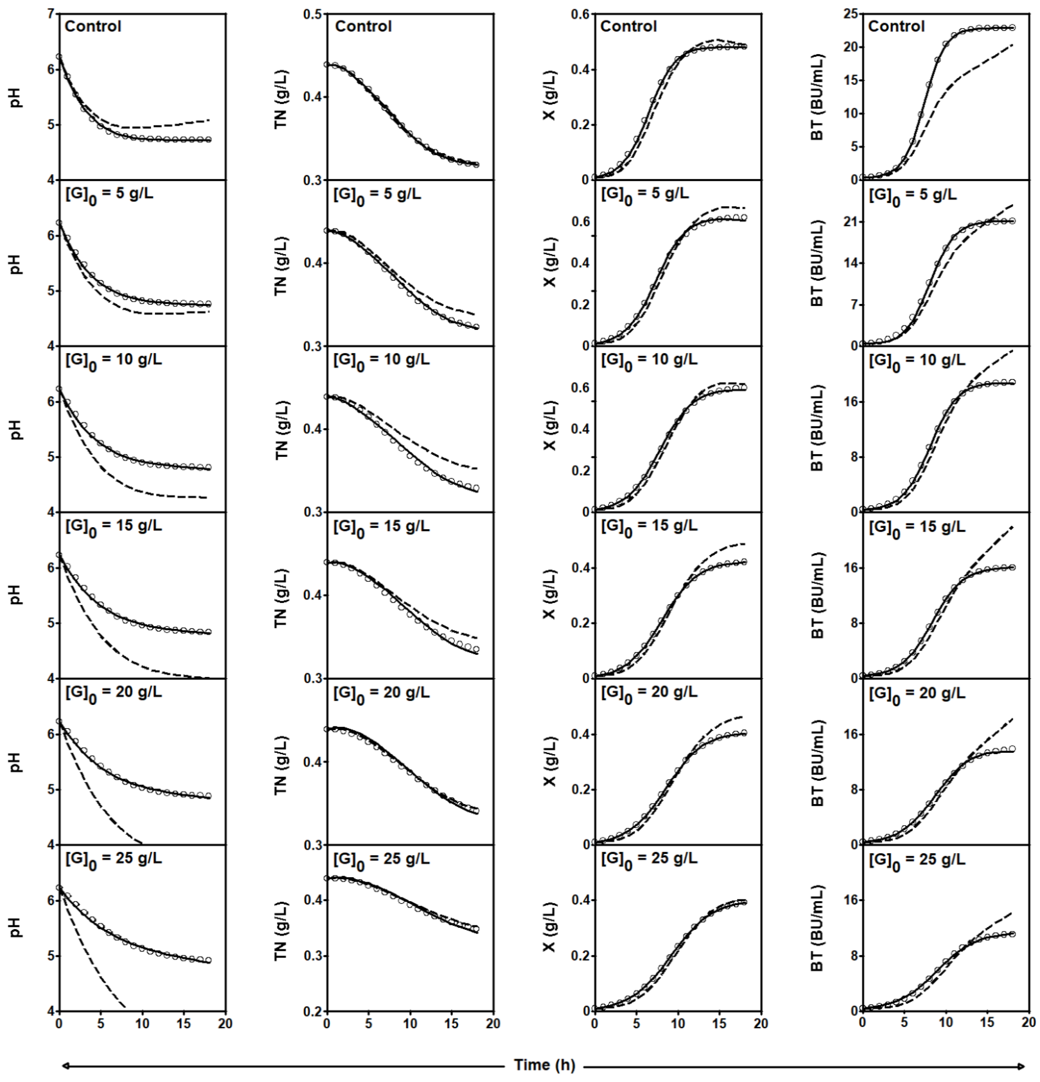
2.3.1. Series of Fermentation DW-G

Table 4 shows the parameter values as well as the statistical analysis obtained when the four-dimensional predator-prey system (1)–(4) was fitted to the experimental data of cultures pH, TN, X, and BT in the DW-G cultures.

In this case, all values of the parameters in Equations (1)–(4) were significant (p < 0.05) and considerably higher values for R_pH² (between 0.9968 and 0.9980), R_TN² (between 0.9987 and 0.9998), R_X² (between 0.9990 and 1.0000), and R_BT² (between 0.9992 and 1.0000) were obtained. In addition, the values of B_f and A_f calculated for Equations (1)–(4) were ~ 1 and the RPDM values were considerably lower than 10% (Table 4). Therefore, it could be considered that the use of the four-dimensional predator-prey system (1)–(4) accurately described the trend observed for the culture pH, TN, X, and BT in the DW-G cultures.

Regarding the equation parameters, it can be noted that the values of a and b in Equation (1) had a negative sign and their absolute values decreased (Table 4). This is because the culture pH drop (the difference between the initial and final pH values) decreased and the final pH increased with the increase in the initial concentration of glucose [G₀] (from 0 to 25 g/L) in the media (Figure 1). In addition, the value of c decreased from 0.039 to 0.002 with the increase in [G₀] due to the inhibition that increasing glucose concentration produced on the growth of L. lactis CECT 539 and, consequently, on lactic acid production [16], causing a gradual reduction in the pH drop in the culture media (Figure 1).

In the case of Equation (2), negative values for d, e, f, and g, and positive values for h were obtained (Table 4). The decrease in the absolute values obtained for d and e could be related to the reduction in the TN consumption rates and the increase in the final TN values observed with the increase in [G₀] (Figure 1). Similarly, the values of f, g, and h were almost similar for all cultures because the TN consumption decreased with the increase in [G₀], in parallel with the reduction in biomass production, nisin synthesis, and pH drop (Figure 1).

Equation (3) also provides an accurate description of biomass production in each culture. In this case, the values of i decreased because of the inhibition that the increasing initial glucose concentrations produced on the growth rate of L. lactis (Figure 1). On the other hand, the value of j did not vary, indicating that the reduction in the growth rate was proportional to the reduction in the maximum biomass concentration produced in the different cultures (Figure 1).

Similarly, a constant value for k was obtained, indicating that the competition between biomass production and nisin synthesis for the nitrogen source was very similar in the different glucose-supplemented cultures. As observed in Figure 1, the reduction in growth caused by the increase in [G₀] was proportional to that observed in nisin synthesis because this bacteriocin was produced in this series of cultures as a pH-dependent primary metabolite [16].

As expected, the values of l and m decreased (Table 4), due to the decrease in the pH drops and TN consumption caused by the reduction in biomass production (Figure 1).

The detailed analysis of the results obtained for Equation (4) showed a decrease in the values of n in agreement with the reduction in nisin production with the increase in [G₀] (Figure 1). The constant value obtained for the o constant could be explained by a proportional decrease in the nisin production rate and maximum nisin levels produced by L. lactis CECT 539. The constant value obtained for p is in perfect agreement with the constant value obtained for k in Equation (3), indicating again that the competition between biomass production and nisin synthesis for the nitrogen source was very similar in the different glucose-supplemented cultures.

The decrease in the values obtained for q could be explained by the fact that the reduction in pH drops with the increase in [G₀] negatively affected the synthesis of nisin. In the unsupplemented culture ([G₀] = 0), the final pH value was 4.73, which is in perfect agreement with the optimum final pH between 4.78 and 4.90 observed in L. lactis cultures in whey [8]. In contrast, a constant value was obtained for r (Table 4), indicating proportional TN consumption for nisin synthesis.

These results corroborate the affirmation that nisin was produced by L. lactis CECT 539 as a pH-dependent primary metabolite [16] and indicate that the TN consumption was proportional to the production of bacteriocin and biomass.

As discussed above, each culture variable (pH, TN, X, and BT) evolved, describing a similar profile in the different fermentations of the DW-G series (Figure 1). However, the rates of culture pH (rpH(t)) and TN (rTN(t)) decreased, and biomass (rX(t)) and nisin (rBT(t)) production in the glucose-supplemented cultures did not exhibit a clear trend compared with the respective rates in the culture in the unsupplemented culture (Figure 5).

From the detailed observation of Figure 5, it can be noted that the highest rpH(t), rX(t), rBT(t)), and rTN(t) were obtained in the unsupplemented DW substrate during the first 4, 8, 9, and 12 h of fermentation, respectively. However, after these times, the four rates in the unsupplemented DW medium were lower than the corresponding rates calculated in the glucose-supplemented cultures.

For this reason, the four-dimensional Equations (1)–(4) could not be modified by including a term for explaining the inhibitory effect of the increase in [G₀] on the rates rpH(t), rTN(t), rX(t), and rBT(t)).

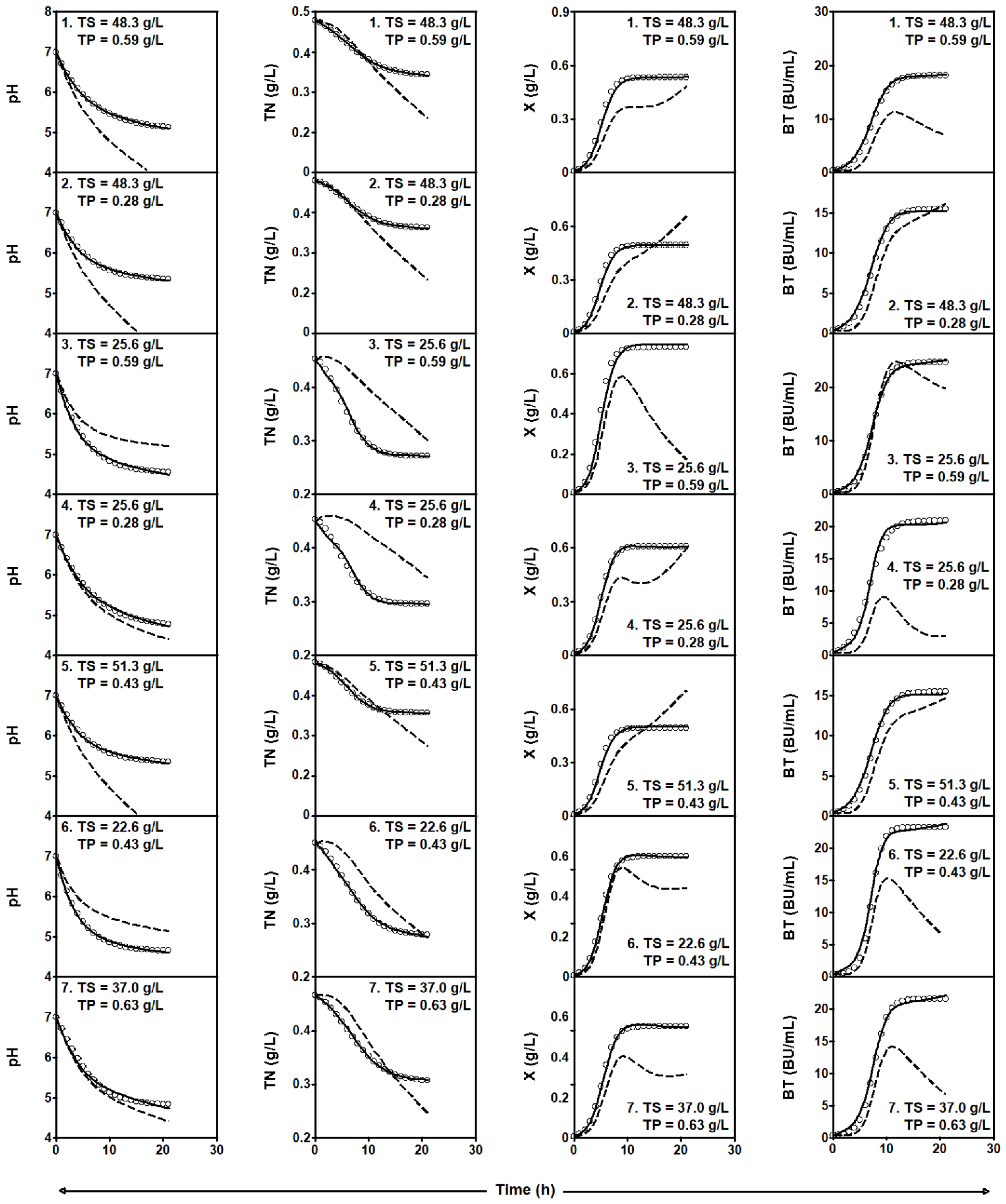
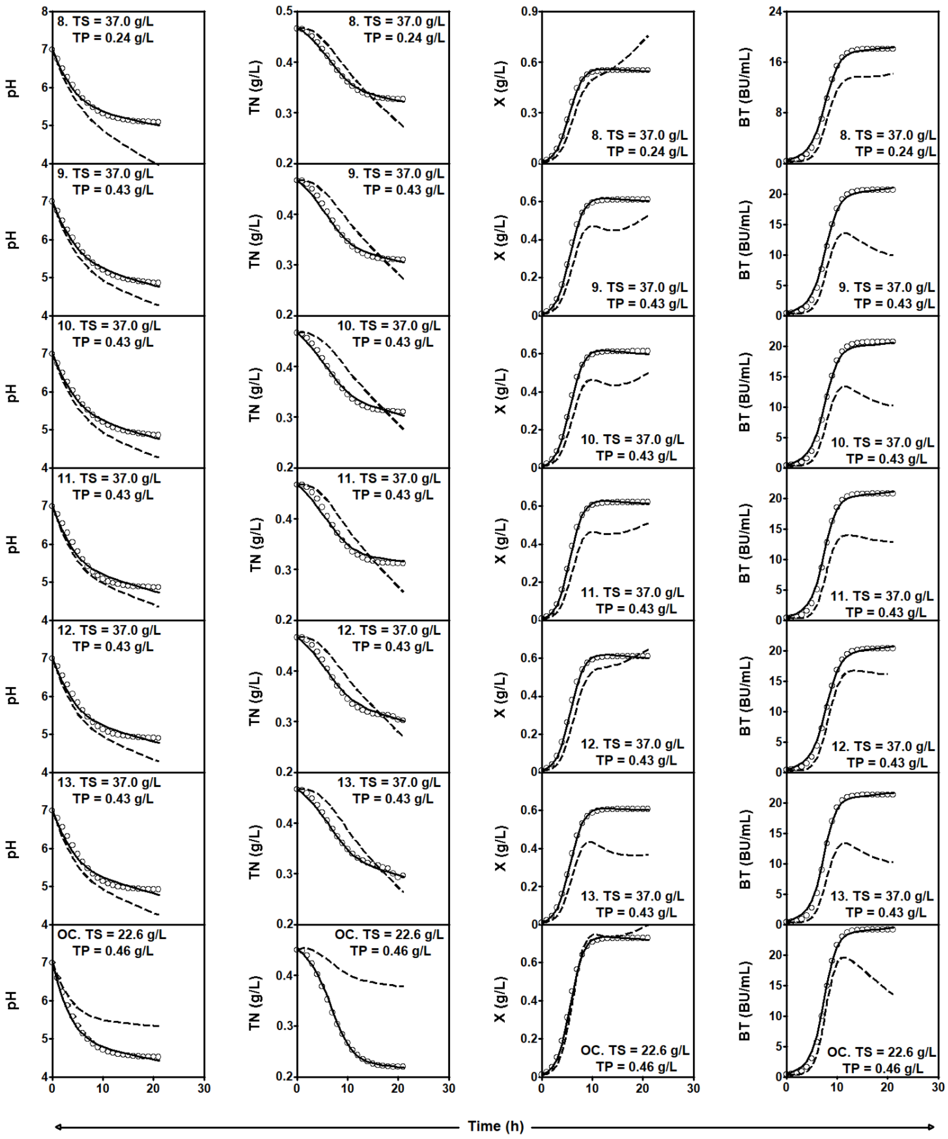
2.3.2. Series of Fermentation DW-TS-TP

Table 5 and Table 6 show the results obtained when the four-dimensional Equations (1)–(4) was fitted to each individual culture of the series of fermentation DW-TS-TP. The predictions of Equations (1)–(4) are shown as solid lines in Figure 2 and Figure 3. As observed before for the series of fermentation DW-G, the DW-TS-TP cultures were satisfactorily described using this modeling procedure (Table 5 and Table 6).

The values of a, b, and c in Equation (1), as expected, depended on the initial chemical composition of the media (mainly the initial concentrations of TS and TP). So that the highest a value was obtained in the culture performed at the optimum conditions (TS = 22.6 g/L, TP = 0.46 g/L, Table 6), in which the highest pH drop (difference between the initial and final pH value) was generated (Figure 2 and Figure 3). The calculated values for b and c varied between 0.007 and 0.013 and between 0.033 and 0.057, respectively (Table 5 and Table 6), which were dependent on the growth of L. lactis in the different cultures (Figure 2 and Figure 3).

The highest values for d and f in Equation (2) were obtained at the optimum conditions (Table 6), in which the highest amounts of TN and biomass were consumed (0.230 g/L) and produced (0.716 g/L), respectively (Figure 2 and Figure 3). This suggests that the total nitrogen source consumption depended on the initial composition of the fermentation medium, as indicated before [2,5,16,17,18]. The value of e depended on the initial media composition, but the values of g and h were constant, indicating a proportional consumption of TN for nisin production and a similar effect of pH on TN assimilation.

The maximum growth rate was observed in the culture performed at TS = 22.60 g/L, TP = 0.46 g/L, and in accordance with this, the highest value for i in Equation (3) was obtained (Table 5 and Table 6). In addition, the values of j and l varied as a function of the initial TS and TP concentrations in the different culture media, but the value of the competition coefficient k was constant in the different cultures, indicating a proportional efficiency of TN utilization for biomass production and nisin synthesis. The constant value calculated for m suggests that the nitrogen source consumption was directly correlated with biomass production.

When Equation (4) was fitted to the experimental data of nisin synthesis, the highest n value was obtained in the culture performed at the optimum conditions (Table 5 and Table 6) due to the highest bacteriocin production rate observed in this culture (Figure 2 and Figure 3). The coefficient o did not show a significant variation since the relationship between the nisin synthesis rates and the maximum bacteriocin levels produced in the cultures was almost constant. Additionally, the coefficients p, q, and r exhibited constant values, suggesting constancy in the competition between biomass and nisin production for the TN source and in the effect of pH and TN consumption on bacteriocin synthesis.

However, in the case of nisin production, the values of RPDM corresponding to some cultures were higher than 10% (Table 5 and Table 6), due to the lack of fit between the experimental and calculated values observed during the first 7 h of fermentation (Figure 2 and Figure 3). This was probably because nisin production was quantified by a photometric bioassay using an indicator strain [16] and, consequently, the experimental error in determining nisin titers could be greater than that of the analytical methods used in pH, total nitrogen, and biomass measurements. So that in nisin determination, the differences between the experimental and predicted values during the first 7 h of fermentation were low (Figure 2 and Figure 3), but the experimental nisin data in this interval, used as the denominator in Equation (8), were also considerably low, increasing the RPDM value (Table 5 and Table 6).

In the series of cultures DW-TS-TP, the effects of the initial TS and TP concentrations on both the growth and bacteriocin production were described by empirical quadratic equations [17]. The inclusion of terms for explaining these effects in the four-dimensional predator-prey system (1)–(4) could contribute to obtaining a general equation for describing the evolution of the four response variables (pH, TN, X, and BT). However, this approach has several drawbacks since too large equations could be obtained, and information about the true relationship between the dependent variables (pH(t), TN(t), X(t), BT(t)), and the own essence of the LV equation would be lost.

In fact, the rates of culture pH drop (rpH), total nitrogen consumption (rTN), and biomass (rX) and nisin (rBT) production in the different experiments (1–14) did not show a clear dependence on changes in initial TS and TP concentrations (Figure 6).

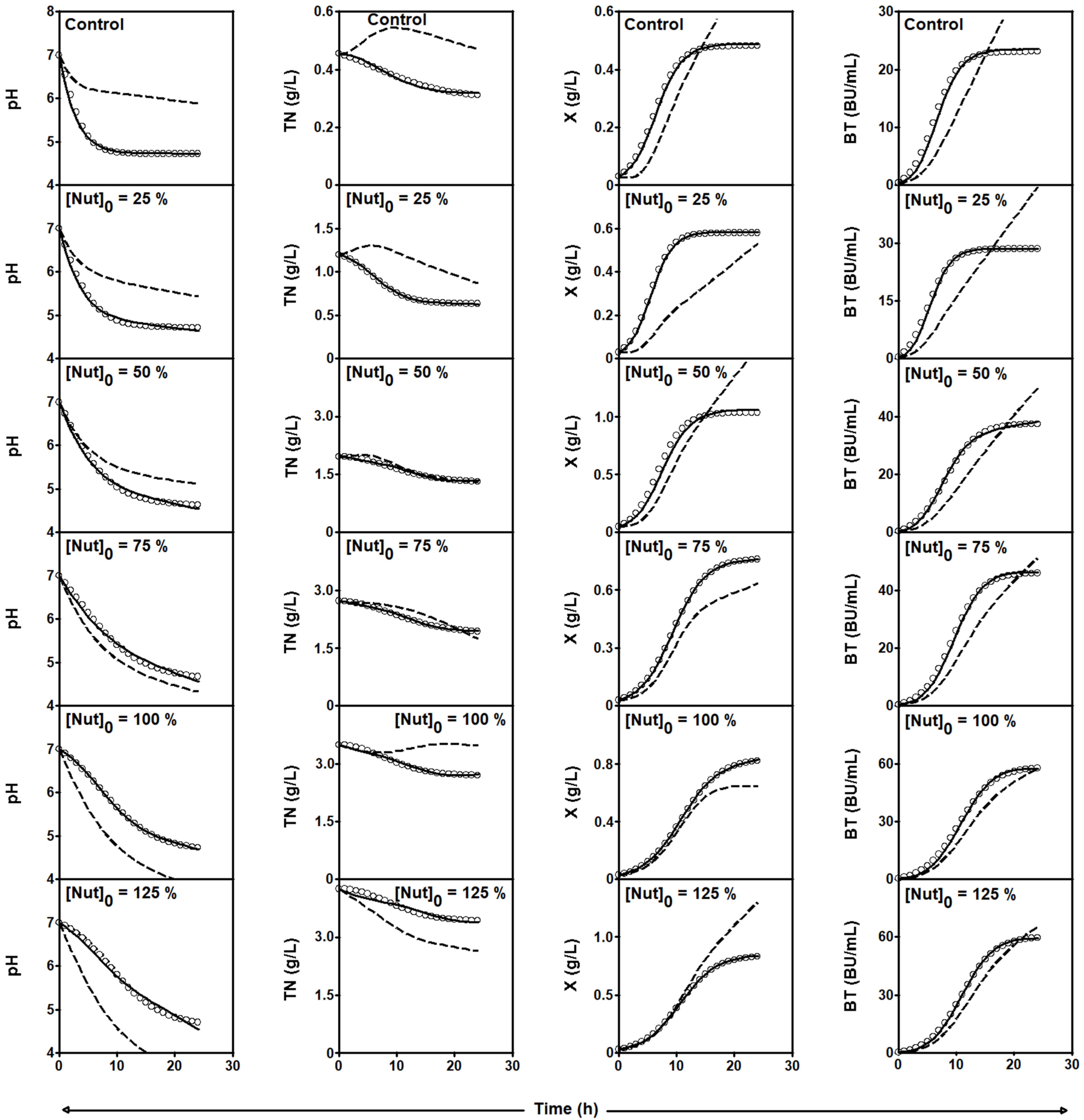
2.3.3. Series of Fermentation DW-MRS

In this series of fermentation, the absolute values of the constant a increased when the DW medium was supplemented with MRS nutrients from 0 to 50% (fermentations DW-MR0%, DW-MRS25%, and DW-MRS50%) since the pH drop increased slightly in these cultures from 2.27 to 2.36 (Table 7, Figure 4). The absolute values of b decreased slightly; meanwhile, the constant c decreased from 0.103 to 0.022 because of the increase in the buffering capacity of media supplemented with increasing MRS nutrient concentrations from 0 to 50% [18]. This counteracted the reduction in pH values due to acid organic production by the nisin-producing strain.

However, the values of a and b had a positive value in the following cultures (fermentations DW-MR75%, DW-MRS100%, and DW-MRS125%), and c increased in DW-MRS100% and DW-MRS125% fermentations. The sign change observed for a and b from negative in the first three fermentations (DW-MR0%, DW-MRS25%, and DW-MRS50%) to positive in the latter three cultures (DW-MR75%, DW-MRS100%, and DW-MRS125%) could be related to the change in the trajectories described by the culture pH. These pH trajectories evolved from convex curves in the first three cultures to inverted S-curves in the three latter cultures (Figure 4).

Thus, the values of a, b, and c increased in the fermentation DW-MRS100% compared to the fermentation DW-MRS75% due to the increase in the growth of L. lactis. However, in the fermentation DW-MRS125%, the increase in the buffering capacity of the supplemented media counteracted the effect of lactic acid production by the growing strain [18]. For this reason, the values of a, b, and c decreased slightly (Table 7).

Regarding Equation (2), it can be noted that the values of d and e (with negative signs) increased and decreased, respectively, from the fermentation DW-MRS0% to DW−75% (Table 7). However, the sign of both constants becomes positive in the following fermentations due to the change in the curvature of the TN trajectories from convex curves (first four cultures) to inverted S-curves (fermentations DW-MRS100% and DW-125%), as observed before for the culture pH curves (Figure 4).

In fermentations DW-MRS0% to DW-75%, the values of f and h increased with nutrient supplementation since the addition of MRS nutrients led to an increase in the TN consumption, growth, and pH gradient. The latter probably affected the TN consumption rate since the consumption of this nutrient depends on the culture pH, as explained above [18,20]. The constant e varied as a function of the value of d and the lowest TN concentration reached in the cultures, and g was approximately constant (−0.009 ± 0.002) in the four fermentations (Table 7). In comparison with fermentation DW-MRS100%, fermentation DW-125% provided higher values of d and e, in agreement with the increase in TN consumption in the latter culture. However, the value of f decreased while those of g and h were constant in both cultures.

Equation (3) provided increasing values for i due to the increase in the growth rates caused by the increase in MRS nutrient supplementation; meanwhile, the value of j depended on the values of i and the maximum biomass level reached in each culture. The values of k (0.007 ± 0.000) and l (0.087 ± 0.002) were almost constant, and m showed an increasing trend.

In Equation (4), the values of n increased with the increase in nutrient supplementation, indicating a stimulation in nisin production, and the values of the constant o varied depending on the values of n and the maximum nisin titers reached in the cultures. In addition, the values of p and r did not vary, but the constant q increased (Table 7), probably because of the changes in the trajectories described by the culture pH that affected the evolution of nisin production in the cultures (Figure 4), as commented above [5,8,12].

In this series of cultures, the increase in the MRS nutrients added into the DW medium affected both the evolution of the culture variables and the final concentrations of biomass and nisin obtained (Figure 4), as well as the rates rpH, rTN, rX, and rBT (Figure 7). The rates of culture pH decrease exhibited a transition from exponential decay-shaped curves (in the DW25, DW50, and DW75 media) to bell-shaped curves (in the DW100 and DW125 media); meanwhile, the rTN, rX, and rBT profiles showed bell-shaped curves [25]. However, the rpH, rTN, rX, and rBT profiles did not show an appreciable relationship (linear, quadratic, sigmoidal, etc.) with the initial MRS nutrient concentration ([Nut]₀) in the medium.

Therefore, in this case, it is also difficult to develop a general four-dimensional predator-prey system describing the evolution of pH, TN, X, and BT as a function of the initial concentrations of MRS nutrients.

2.4. Mathematical Analysis of the Four-Dimensional Lotka–Volterra Equation

After demonstrating the feasibility of the designed four-dimensional Lotka–Volterra equation to describe the batch nisin production system in different batch cultures, the following step was focused on the mathematical study of the equation by determining its approximate solutions and analyzing its equilibrium points and trajectories around the stable equilibrium points.

2.4.1. Generalized Four-Dimensional Lotka–Volterra Equation

Given two column vectors of ${ℝ}^n$, x, and y, their component-by-component product can be defined by the following:

$$x·y=\left[\begin{array}{c}{x}_1{y}_1\\ x_2{y}_2\\ ⋮\\ x_n{y}_n\end{array}\right]$$

Given $x\in {ℝ}^{\mathrm{n}}$ and $A\in {\mathrm{M}}_{\mathrm{n}\times \mathrm{n}}\left(ℝ\right)$ we define the following:

$$A·x=\left[\begin{array}{c}{x}_1{A}_1\\ x_2{A}_2\\ \begin{array}{c}⋮\\ x_n{A}_n\end{array}\end{array}\right]$$

where A_i is the i-th row of the matrix A.

The generalized Lotka–Volterra equations are given by the system of differential equations given by the following:

$$x^{\prime }=x·\left(b-Ax\right)$$

where b is a column vector and A is a square matrix.

Lemma 1.

Suppose A is nonsingular. The Jacobian of $F\left(x\right)=x·\left(b-Ax\right)$satisfies the following:

$$J_F\left(\tilde{x}\right)=-A·\tilde{x}$$

$$\mathrm{for} \tilde{x}=A^{-1}b.$$

Proof. 

Note that

$$F_i=\left(b_i-{\displaystyle \sum }_{j=1}^n{a}_{ij}{x}_j\right)x_i$$

where it follows that

$$\nabla F_i\left(x\right)=\left(-a_{i1}{x}_i,-a_{i2}{x}_i,\dots ,-a_{i,i-1}{x}_i,-a_{ii}{x}_i+b_i-{\displaystyle \sum }_{j=1}^n{a}_{ij}{x}_j,-a_{i,i+1}{x}_i,\dots ,-a_{in}{x}_i\right)$$

Thus,

$$\nabla F_i\left(\tilde{x}\right)=\left(-a_{i1}{\tilde{x}}_i,-a_{i2}{\tilde{x}}_i,\dots ,-a_{i,i-1}{\tilde{x}}_i,-a_{ii}{\tilde{x}}_i,-a_{i,i+1}{\tilde{x}}_i,\dots ,-a_{i,n}{\tilde{x}}_i\right)=-{\tilde{x}}_i{A}_i$$

which proves the Lemma 1. □

As a consequence of the above lemma and the linearization theorem of Liapunov and Poincaré, the following theorem follows:

Theorem 1.

If A is nonsingular, the generalized Lotka–Volterra equations have a unique equilibrium point with all their entries different from zero, given by$\tilde{x}=A^{-1}b$. If, in addition, the matrix$A·\tilde{x}$has all its eigenvalues with a positive real part, then$\tilde{x}$is asymptotically stable [26]. Note that, since $J_F\left(\tilde{x}\right)=-A·\tilde{x}$ that corresponds to the situation in which all the eigenvalues of the Jacobian have a negative real part.

2.4.2. Numerical Analysis

To perform the mathematical analysis of the four-dimensional LV-like equation designed in this work, we use the experimental data corresponding to the unsupplemented (first) culture of the DW-G series (Table 4). So that the analysis was carried out considering the following parameter values of: a = −0.154, b = −0.037, c = 0.039, d =−0.194, e = −0.909, f = −0.066, g = −0.002, h = 0.034, i = 0.843, j = 0.787, k = 0.008, l = 0.066, m = −0.104, n = 3.727, o = 0.036, p = 0.137, q = 0.607, and r = −0.092.

An interactive environment of MATLAB (app designer) from the function ode45.m was developed to obtain approximate solutions to the four-dimensional LV-like equation for the desired initial conditions. In particular, for each equilibrium point p(p₁,p₂,p₃,p₄) and ε = (ε₁,ε₂,ε₃,ε₄), the approximate solutions x_ε(t), y_ε(t), z_ε(t), and w_ε(t), corresponding to the following initial conditions: x₀ = p₁ + ε₁, y₀ = p₂ + ε₂, z₀ = p₃+ ε₃, w₀ = p₄ + ε₄, can be calculated. Figure 8 shows the graphs corresponding to x_ε(t), y_ε(t), z_ε(t), and w_ε(t) for 40 random values of ε in the 4-dimensional sphere with the center at the origin and a radius of 0.01.

The equilibrium points (pH(t), TN(t), X(t), and BT(t)) corresponding to the four-dimensional Lotka–Volterra equation were obtained by solving $\mathit{x}·\left(\mathit{b}-\mathit{A}\mathit{x}\right)=0,$ where:

$$\mathit{x}=\left[\begin{array}{c}pH\\ TN\\ \begin{array}{c}X\\ BT\end{array}\end{array}\right], \mathit{b}=\left[\begin{array}{c}-a\\ -d\\ \begin{array}{c}i\\ n\end{array}\end{array}\right], \mathit{A}=\left[\begin{array}{c}-b\\ -h\\ \begin{array}{c}l\\ q\end{array}\end{array} \begin{array}{c}0\\ -e\\ \begin{array}{c}m\\ r\end{array}\end{array} \begin{array}{c}-c\\ -f\\ \begin{array}{c}j\\ p\end{array}\end{array} \begin{array}{c}0\\ -g\\ \begin{array}{c}k\\ o\end{array}\end{array}\right]$$

With this procedure, the following 16 equilibrium points were calculated: P₁(0.000,0.000,0.000,0.000), P₂(0.000,0.000,1.071,0.000), P₃(0.000,0.000,0.000,103.528), P₄(0.000,0.000,0.019,103.453), P₅(0.000,0.213,0.000,0.000), P₆(0.000,−0.014,0.000,103.491), P₇(0.000,0.134,1.089,0.000), P₈(0.000,−0.015,0.018,103.420), P₉(4.162,0.000,0.000,0.000), P₁₀(4.162,0.000,0.000,33.349), P₁₁(4.162,0.369,0.000,0.000), P₁₂(4.162,0.294,0.000,34.101), P₁₃(4.861,0.000,0.663,0.000), P₁₄(4.627,0.000,0.441,23.837), P₁₅(4.906,0.346,0.705,0.000), and P₁₆(4.665,0.301,0.477,23.812).

Of all, only the point P₁₆ (4.665,0.301,0.477,23.812) has biological interest since the other equilibrium points contain at least one zero, and this implies that there are no viable cells (X = 0), nitrogen source (TN = 0), or nisin (BT = 0), or that the culture pH reached the value zero. However, in the fermentation analyzed, this was not possible because during the incubation, the culture variables were all greater than zero during the incubation period (Figure 1). At the beginning of fermentation, the values of the culture pH, [TN], [X], and [BT] were 6.230, 0.439 g/L, 0.010 g/L, and 0.430 BU/mL, respectively, and reached the final values of 4.730, 0.319 g/L, 0.480 g/L, 22.897 BU/mL, respectively.

So that, the unique equilibrium point (P₁₆) with all its components different from zero is as follows:

$$\tilde{x}=A^{-1}b=\left[\begin{array}{c}4.665\\ 0.301\\ \begin{array}{c}0.477\\ 23.812\end{array}\end{array}\right]$$

That satisfies:

$$A·\tilde{x}=\left[\begin{array}{c}0.1726\\ -0.0102\\ \begin{array}{c}0.0315\\ 14.4542\end{array}\end{array} \begin{array}{c}0\\ 0.2735\\ \begin{array}{c}-0.0497\\ -2.1907\end{array}\end{array} \begin{array}{c}-0.1819\\ 0.0198\\ \begin{array}{c}0.3759\\ 3.2623\end{array}\end{array} \begin{array}{c}0\\ 0.0006\\ \begin{array}{c}0.0038\\ 0.8572\end{array}\end{array}\right]$$

The eigenvalues of this matrix are 0.4096, 0.2875, 0.8494, and 0.1327. By the previous Theorem, $\tilde{x}$ is asymptotically stable.

Figure 9 shows how the calculated trajectories of the four culture variables evolve from different initial values to converge to their corresponding equilibrium point (pH = 4.665, TN = 0.301 g/L, X = 0.477 g/L, BT = 23.812 BU/mL).

As observed in Figure 9B, the four culture variables (pH, TN, X, and BT) gradually reach a plateau phase and stabilize at the above-mentioned stable equilibrium point. In fact, the coordinates of the latter point are in perfect agreement with the experimental values of the culture variables (pH = 4.730, TN = 0.319 g/L, X = 0.482 g/L, BT = 22.905 BU/mL) obtained after 17 h of incubation, from which the culture variables stabilized (Figure 1).

The phase graphs (Figure 10) show that there is an interaction between the four culture variables over time. Thus, the relationships between TN vs. pH and BT vs. X were directly proportional because TN concentration decreased with the decrease in pH, and BT increased with the growth of L. lactis since this bacteriocin was produced in the logarithmic phase of growth as a primary metabolite (Figure 1).

In contrast, the relationships X vs. pH, BT vs. pH, X vs. TN, and BT vs. TN were inversely proportional because the biomass and nisin synthesis increased with the decrease in pH and increase in TN consumption, which reduced the concentration of the nitrogen source (Figure 1).

On the other hand, closed elliptic orbits previously observed in classic predator-prey models were not observed when the four-dimensional LV-like equation was used to describe the batch nisin system, because these microbial relationships are not periodic, as those of the populations of predators and prey in biological systems [27].

2.4.3. Study of the Parameter Values for Which There Is an Asymptotically Stable Solution

In what follows, we will establish, by means of a Monte Carlo study [28,29], which conditions must be satisfied by the parameters defining the matrix A and the vector b so that the Lotka–Volterra equation has a single asymptotically stable equilibrium point with all its positive (and non-zero) coordinates.

If we denote by ${\left\{p_i\right\}}_{i=1}^{18}$ the generic parameters (i.e., a,b,c,d,e,f,g,h,i,j,k,l,m,n,o,p,q,r), and by ${\left\{p_{i0}\right\}}_{i=1}^{18}$ the current parameters, the aim of our study is to look for positive values, R₁ and R₂, as large as possible, so that if

p_i ∈ [p_i0 (1-R₁), p_i0 (1+R₂)] (if p_i 0 ≥ 0)

p_i ∈ [p_i0 (1+R₂), p_i0 (1-R₁)] (if p_i 0 < 0) being i = 1,2,…,18

Then $\tilde{x}={\mathit{A}}^{-1}\mathit{b}$ satisfies that all its entries are positive and the matrix $\mathit{A}·\tilde{x}$ has all its eigenvalues with a positive real part.

For this purpose, we fixed R₁, and the step h = 0.001, and we determined the first value of a natural k such that if R₂ =k·h, and 10.000 random values were taken for each one of the intervals $\left[p_{i0}\left(1-R_1\right), p_{i0}\left(1+R_2\right)\right]$ (if p_i 0 ≥ 0) and $\left[p_{i0}\left(1+R_2\right), p_{i0}\left(1-R_1\right)\right]$ (if p_i 0 < 0), then $\tilde{x}={\mathit{A}}^{-1}\mathit{b}$ has any of its entries nonpositive or the matrix $\mathit{A}·\tilde{x}$ has some eigenvalue with a nonpositive real part.

We observed that if R₁ > 0.12, there are no asymptotically stable equilibrium points with all their non-zero coordinates. The left and right parts of Figure 11 show the curve R₁ → R₂ and the curves R₁ → 1 − R₁ and R₁ → 1 + R₂, respectively. As can be observed in these figures, the range of the parameters’ validity is approximately equal to $0.12\left|p_{i0}\right|$, i = 1,2,…,18.

3. Materials and Methods

3.1. Microorganisms, Culture Media, and Inoculum Preparation

In this work, Lactococcus lactis CECT 539 and Carnobacterium piscicola CECT 4020 were used as the nisin-producing strain and target bacterium (in the nisin activity bioassay), respectively. Both strains were obtained from the Spanish Type Culture Collection (CECT) and cultured at 30 °C in MRS (de Man, Rogosa and Sharpe) agar slants or broth.

Diluted whey (DW) and concentrated mussel-processing waste (CMPW) were used to prepare the different culture media (Table 1). Sterilization (121 °C/15 min) of these substrates led to the precipitation of a protein fraction that interfered with biomass measurements. For this reason, the precipitated material was removed by acidification of the DW and CMPW substrates to pH 4.5 with 5 N HCl, heating (121 °C/15 min) and centrifugation (12,000 × g for 15 min) [16,17,18].

Given that the nisin-producing strain is not an amylolytic bacterium, the glycogen contained in the CMPW was enzymatically hydrolyzed to produce a glucose-containing substrate as described in Costas et al. [17].

To prepare the different fermentation substrates, DW medium was supplemented with the following nutrients: (i) different amounts of glucose to obtain 5, 10, 15, 20, and 25 g glucose/L of medium (series of fermentation DW-G) [16], (ii) different volumes of CMPW medium (101.33 g glucose/L) and amounts of KH₂PO₄ to obtain initial total sugars and phosphorous concentrations between 22.61 and 51.35 g/L, and 0.24 and 0.63 g/L, respectively (series of fermentation DW-TS-TP) [17], and (iii) MRS broth nutrients (except glucose and Tween 80) at 25, 50, 75, 100, and 125% (w/v) of their standard concentrations in the complex substrate to produce the DW25, DW50, DW75, DW100, and DW125 media (series of fermentation DW-MRS) [18]. In these three series of fermentation, control cultures in unsupplemented DW medium were performed to obtain data for the comparisons [16,17,18].

Table 1 and Table 2 show the mean compositions of the resulting culture media used in this work.

To prepare the preculture, cells of L. lactis CECT 539 from MRS agar slants were used to inoculate sterile MRS broth (10 mL) and incubated at 30 °C for 12 h with shaking at 200 rpm. After that, 50 mL of inoculum medium (which was, in each case, similar to the corresponding fermentation substrate) were inoculated with 1 mL of the preculture and subsequently incubated for 12 h at 30 °C with shaking at 200 rpm. An appropriate volume of the latter culture was used to inoculate the corresponding fermentation medium used in the different batch cultures to give an initial viable cell count of 1.5 × 10⁹ colony-forming units/mL [16,17,18].

3.2. Batch Cultures

The different experimental data used in this research were collected from previous batch cultures of L. lactis CECT 539 [16,17,18]. The fermentations were conducted in duplicate in 250 mL Erlenmeyer flasks that contained 50 mL of the corresponding DW-based medium. After inoculation, the flasks were incubated at 30 °C with shaking at 200 rpm for 18 h [16], 21 h [17], and 24 h [18].

3.3. Analytical Methods

The corresponding analytical methods used to measure culture pH and concentrations of total nitrogen, biomass, and nisin were previously described in Costas et al. [16].

3.4. Statistical Significance of the Parameters and Equation

Before being used to fit the four-dimensional predator-prey system, the experimental data of the culture pH and remaining concentrations of total nitrogen, biomass, and nisin [16,17,18] were smoothed using the following logistic equations (5–7):

For the culture pH (Q(t) = pH(t)) and total nitrogen (Q(t) = TN(t)) decrease, we modified the logistic decline equation presented by Goudar et al. [28] as follows:

$$Q\left(t\right)=\frac{A}{B-e^{\left(C_0+C_1·t+C_2·t^2\right)}}$$

(5)

Being $A=\frac{p{H}_0·p{H}_f}{p{H}_0-p{H}_f}$ for culture pH or $A=\frac{T{N}_0·T{N}_f}{T{N}_0-T{N}_f}$ for TN.

and $B=\frac{p{H}_0}{p{H}_0-p{H}_f}$ for culture pH or $B=\frac{T{N}_0}{T{N}_0-T{N}_f}$ for TN.

For biomass (X(t)) production, the logistic equation presented by Goudar et al. [30] was used by considering that the death cell rate was zero, as follows:

$$X\left(t\right)=\frac{D}{1+E·e^{-F·t}}$$

(6)

Being $D=X_{max}$ and $E=\frac{X_{max}-X_o}{X_o}$.

For nisin (BT(t)) synthesis, we modified the logistic decline equation [30] as follows:

$$BT\left(t\right)=\frac{G}{1+H·e^{\left(-I·t\right)}}-\frac{G}{1+H}$$

(7)

Being $G=B{T}_{max}$.

In this work, the values of the different constants were first obtained by numerical integration of the four differential equations (dpH(t)/dt, dTN(t)/dt, dX(t)/dt, and dBT(t)/dt) of the competitive predator-prey system (1)–(4), minimizing the sum of quadratic differences between equation-predicted and experimental values, with the non-linear least squares (quasi-Newton) method included in the Solver tool of Microsoft Excel 2016 spreadsheet. Then, the values and statistical significance (p < 0.05) of both the constants and the four-dimensional Lotka–Volterra-like equation were corroborated with an accurate statistical analysis using the statistics software SigmaPlot for Windows version 12.0 (Systat Software, Inc., San Jose, CA, USA, 2012) and the Regression (non-lineal) module of the software package IBM SPSS Statistics 20.0 for Windows (Release 20.0.1; SPSS Inc., Chicago, IL, USA, 2021). The significance of the different constants in each differential equation was evaluated by using Student’s t-test and considering the corresponding p values [31] for each constant. Thus, the values of the constants with a high t-value and a p value lower than 0.05 were considered statistically significant. The significance of the different constants in each differential equation was evaluated by using Student’s t-test and considering the corresponding p values for each constant. The convergence of the parameters was checked by using the Levenberg–Marquardt method [32,33] of the Regression (non-lineal) module of the software package IBM SPSS Statistics 20.0 for Windows (Release 20.0.1; SPSS Inc., Chicago, IL, USA, 2021).

The global consistency of the four differential equations was verified by using the overall Fisher’s F-test (α = 0.05) and considering the corresponding p values for each equation. Thus, a high F-value and a p value lower than 0.05 means that the differential equation was statistically significant.

The goodness-of-fit of the four differential equations was also checked using the mean relative percentage deviation modulus (RPDM) values [5] and the bias (B_f) and accuracy (A_f) factors [34]:

$$RPDM=\frac{100}{n}\sum \left|\frac{Yex{p}_i-Ypre{d}_i}{Yex{p}_i}\right|$$

(8)

$$B_f={10}^{\frac{\sum log(\frac{Ypre{d}_i}{Yex{p}_i})}{s}}$$

(9)

$$A_f={10}^{\frac{\sum \left|log(\frac{Ypre{d}_i}{Yex{p}_i})\right|}{s}}$$

(10)

where s is the number of experimental data, Yexp_i is the experimental value and Ypred_i is the value predicted by the equation. Values of R² ≥ 0.95, RPDM < 10% [5], and B_f and A_f close to 1 [34] indicate that the corresponding equation was accurately fitted to the experimental data.

3.5. Mathematical Analysis

The mathematical analysis of the four-dimensional Equation (Equations (1)–(4)) was performed with the MATLAB Runtime R2021a (MathWorks Inc., Natick, MA, USA) using the values of the constants corresponding to the unsupplemented culture of the DW-G series.

4. Conclusions

The main contribution of this paper is the development and mathematical analysis, for the first time, of a four-dimensional predator-prey system for an accurate description of the batch nisin production system by L. lactis CECT 539 in different series of fermentation in DW media supplemented with different concentrations of glucose (DW-G cultures), total sugars and phosphorous (DW-TS-TP cultures), or MRS broth nutrients (DW-MRS cultures).

The results obtained in this paper demonstrated that the microbiological bacteriocin production system could be explained by considering the biological approach used to describe the relationships between species that compete for the same nutrient sources. Thus, further knowledge is provided about the relationship between the main culture variables (culture pH, total nitrogen consumption, and the synthesis of biomass and bacteriocin) involved in nisin production, which is usually difficult to explain.

The mathematical novelty of this paper relies on the determination, for the first time, of the equilibrium points and trajectories around the stable equilibrium point obtained from the mathematical analysis of the four-dimensional model designed in this paper. Thus, the existence of an asymptotically stable equilibrium point with biological sense (pH = 4.665, TN = 0.301 g/L, X = 0.477 g/L, BT = 23.812 BU/mL), to which the culture evolved to reach the stationary state, was proved. The existence of this equilibrium point is in perfect agreement with the experimental point (pH = 4.730, TN = 0.319 g/L, X = 0.482 g/L, BT = 22.905 BU/mL at 17 h of fermentation), from which the four culture variables stabilized.

References

1. Delves-Broughton, J. Nisin. In Encyclopedia of Food Microbiology, 2nd ed.; Robinson, R., Batt, C.A., Tortorello, M.L., Eds.; Academic Press: London, UK, 2014; pp. 187–193. [Google Scholar]
2. Leroy, F.; De Vuyst, L. Growth of the bacteriocin-producing Lactobacillus sakei strain CTC 494 in MRS broth is strongly reduced due to nutrient exhaustion: A nutrient depletion model for the growth of lactic acid bacteria. Appl. Environ. Microbiol. 2001, 67, 4407–4413. [Google Scholar] [CrossRef] [PubMed] [Green Version]
3. van Impe, J.F.; Poschet, F.; Geeraerd, A.H.; Vereecken, K.M. Towards a novel class of predictive microbial growth models. Int. J. Food Microbiol. 2005, 100, 97–105. [Google Scholar] [CrossRef] [PubMed]
4. Wachenheim, D.E.; Patterson, J.A.; Ladisch, M.R. Analysis of the logistic function model: Derivation and applications specific to batch cultured microorganisms. Bioresour. Technol. 2003, 86, 157–164. [Google Scholar] [CrossRef]
5. Guerra, N.P.; Torrado, A.; López, C.; Fajardo, P.; Pastrana, L. Dynamic mathematical models to describe the growth and nisin production by Lactococcus lactis subsp. lactis CECT 539 in both batch and re-alkalized fed-batch cultures. J. Food Eng. 2007, 82, 103–113. [Google Scholar]
6. Vázquez, J.A.; Murado, M.A. Unstructured mathematical model for biomass, lactic acid and bacteriocin production by lactic acid bacteria in batch fermentation. J. Chem. Technol. Biotechnol. 2008, 83, 91–96. [Google Scholar] [CrossRef] [Green Version]
7. Shirsat, N.; Mohd, A.; Whelan, J.; English, N.J.; Glennon, B.; Al-Rubeai, M. Revisiting Verhulst and Monod models: Analysis of batch and fed-batch cultures. Cytotechnology 2015, 67, 515–530. [Google Scholar] [CrossRef] [Green Version]
8. Guerra, N.P. Modeling the batch bacteriocin production system by lactic acid bacteria by using modified three-dimensional Lotka–Volterra equations. Biochem. Eng. J. 2014, 88, 115–130. [Google Scholar] [CrossRef]
9. Callewaert, R.; De Vuyst, L. Bacteriocin production with Lactobacillus amylovorus DCE 471 is improved and stabilized by fed-batch fermentation. Appl. Environ. Microbiol. 2000, 66, 606–613. [Google Scholar] [CrossRef] [Green Version]
10. Wick, L.M.; Weilenmann, H.; Egli, T. The apparent clock-like evolution of Escherichia coli in glucose-limited chemostats is reproducible at large but not at small population sizes and can be explained with Monod kinetics. Microbiology 2002, 148, 2889–2902. [Google Scholar] [CrossRef] [Green Version]
11. Luedeking, R.; Piret, E.L. A kinetic study of the lactic acid fermentation. Batch process at controlled pH. J. Biochem. Microbiol. Technol. Eng. 1959, 1, 393–412. [Google Scholar] [CrossRef]
12. Cabo, M.L.; Murado, M.A.; González, M.P.; Pastoriza, L. Effects of aeration and pH gradient on nisin production: A mathematical model. Enzym. Microb. Technol. 2001, 29, 264–273. [Google Scholar] [CrossRef]
13. Constandinides, K.; Damianou, P.A. Lotka–Volterra equations in three dimensions satisfying the Kowalevski-Painlevé property. Regul. Chaotic Dyn. 2011, 16, 311–328. [Google Scholar] [CrossRef]
14. Yang, R.; Ray, B. Factors influencing production of bacteriocins by lactic acid bacteria. Food Microbiol. 1994, 11, 281–291. [Google Scholar] [CrossRef]
15. Wang, R.; Xiao, D. Bifurcations and chaotic dynamics in a 4-dimensional competitive Lotka–Volterra system. Nonlinear Dyn. 2010, 59, 411–422. [Google Scholar] [CrossRef]
16. Costas, M.; Alonso, E.; Guerra, N.P. Nisin production in realkalized fed-batch cultures in whey with feeding with lactose- or glucose-containing substrates. Appl. Microbiol. Biotechnol. 2016, 100, 7899–7908. [Google Scholar] [CrossRef]
17. Costas, M.; Alonso, E.; Outeiriño, D.; Guerra, N.P. Production of a highly concentrated probiotic culture of Lactococcus lactis CECT 539 containing high amounts of nisin. 3-Biotech 2018, 8, 292. [Google Scholar]
18. Costas, M.; Alonso, E.; Bazán, D.L.; Bendaña, R.J.; Guerra, N.P. Batch and fed-batch production of probiotic biomass and nisin in nutrient-supplemented whey media. Braz. J. Microbiol. 2019, 50, 915–925. [Google Scholar]
19. Urbansky, E.T.; Schock, M.R. Understanding, deriving, and computing buffer capacity. J. Chem. Educ. 2000, 77, 1640–1644. [Google Scholar] [CrossRef]
20. Poolman, B.; Konings, W.N. Relation of growth of Streptococcus lactis and Streptococcus cremoris to amino acid transport. J. Bacteriol. 1988, 170, 700–707. [Google Scholar] [CrossRef] [Green Version]
21. Abbasiliasi, S.; Tan, J.S.; Ibrahim, T.A.T.; Bashokouh, F.; Ramakrishnan, N.R.; Mustafa, S.; Arif, A.B. Fermentation factors influencing the production of bacteriocins by lactic acid bacteria: A review. RSC Adv. 2017, 7, 29395–29420. [Google Scholar] [CrossRef]
22. Salaün, F.; Mietton, B.; Gaucheron, F. Buffering capacity of dairy products. Int. Dairy J. 2005, 15, 95–109. [Google Scholar] [CrossRef]
23. Parente, E.; Ricciardi, A.; Addario, G. Influence of pH on growth and bacteriocin production by Lactococcus lactis subsp. lactis 14ONWC during batch fermentation. Appl. Microbiol. Biotechnol. 1994, 41, 388–394. [Google Scholar] [CrossRef]
24. van Niel, E.W.J.; Hahn-Hägerdal, B. Nutrient requirements of lactococci in defined growth media. Appl. Microbiol. Biotechnol. 1999, 52, 617–627. [Google Scholar] [CrossRef] [Green Version]
25. Moret-Tatay, C.; Gamermann, D.; Navarro-Pardo, E.; Fernández de Córdoba, P. ExGUtils: A python package for statistical analysis with the ex-gaussian probability density. Front. Psychol. 2018, 9, 612. [Google Scholar] [CrossRef] [Green Version]
26. Hsu, S.-B.; Ruan, S.; Yang, T.-H. Analysis of three species Lotka–Volterra food web models with omnivory. J. Math. Anal. Appl. 2015, 426, 659–687. [Google Scholar] [CrossRef]
27. Adamu, H.A. Mathematical analysis of predator-prey model with two preys and one predator. Int. J. Eng. Appl. Sci. 2018, 5, 17–23. [Google Scholar]
28. Castro-Palacio, J.C.; Isidro, J.M.; Navarro-Pardo, E.; Velázquez-Abad, L.; Fernández-de-Córdoba, P. Monte Carlo Simulation of a modified Chi distribution with unequal variances in the generating gaussians. A Discrete Methodology to Study Collective Response Times. Mathematics 2021, 9, 77. [Google Scholar] [CrossRef]
29. Ortigosa, N.; Orellana-Panchame, M.; Castro-Palacio, J.C.; Fernández de Córdoba, P.; Isidro, J.M. Monte Carlo simulation of a modified Chi distribution considering asymmetry in the generating functions: Application to the Study of Health-Related Variables. Symmetry 2021, 13, 924. [Google Scholar] [CrossRef]
30. Goudar, C.T.; Joeris, K.; Konstantinov, K.B.; Piret, J.M. Logistic equations effectively model mammalian cell batch and fed-batch kinetics by logically constraining the fit. Biotechnol. Prog. 2005, 21, 1109–1118. [Google Scholar] [CrossRef] [PubMed]
31. Tomás Miguel, J.M.; Meléndez Moral, J.C.; Navarro Pardo, E. Factorial confirmatory models of Ryff’s scales in a sample of elderly people. Psicothema 2008, 20, 304–310. [Google Scholar] [PubMed]
32. Kanzow, C.; Yamashita, N.; Fukushima, M. Levenberg–Marquardt methods with strong local convergence properties for solving nonlinear equations with convex constraints. J. Comput. Appl. Math. 2004, 172, 375–397. [Google Scholar] [CrossRef] [Green Version]
33. Behling, R.; Gonçalves, D.S.; Santos, S.A. Local convergence analysis of the Levenberg-Marquardt framework for nonzero-residue nonlinear least-squares problems under an error bound condition. J. Optim. Theory Appl. 2019, 183, 1099–1122. [Google Scholar] [CrossRef]
34. Vazquez, J.A.; Lorenzo, J.M.; Fuciños, P.; Franco, D. Evaluation of non-linear equations to model different animal growths with mono and bisigmoid profiles. J. Theor. Biol. 2012, 314, 95–105. [Google Scholar] [CrossRef] [PubMed]
Figure 1. Experimental data (symbols) of culture pH, TN consumption, and X and Nis synthesis by L. lactis CECT 539 in batch fermentations in DW medium supplemented with different glucose levels ([G]0). Dashed lines drawn through the experimental data are predictions of the global four-dimensional predator-prey system (1)–(4) obtained with the parameters shown in Table 3. Solid lines were obtained by adjusting the four-dimensional predator-prey system to the experimental data corresponding to each individual culture (see parameter values in Table 4). Reproduced with permission from Costas et al. [16], Appl. Microbiol. Biotechnol.; published by Springer Nature, 2016.
Mathematics 10 00677 g001
Figure 2. Experimental data (symbols) of culture pH, TN consumption, and X and Nis production by L. lactis CECT 539 in the first seven batch cultures of the experimental matrix (Table 2), corresponding to the fermentation series DW-TS-TP. Dashed lines drawn through the experimental data are predictions of the global four-dimensional predator-prey systems (1)–(4) obtained with the parameters shown in Table 3. Solid lines were obtained by adjusting the four-dimensional predator-prey system (1)–(4) to the experimental data corresponding to each individual culture (see parameter values in Table 5). Reproduced with permission from Costas et al. [17], 3-Biotech; published by Springer Nature, 2018.
Mathematics 10 00677 g002
Figure 3. Experimental data (symbols) of culture pH, TN consumption, and X and Nis production by L. lactis CECT 539 in the last six batch cultures of the experimental matrix (Table 2) and in the optimum conditions (OC), corresponding to the fermentation series DW-TS-TP. Dashed lines drawn through the experimental data are predictions of the global four-dimensional predator-prey system (1)–(4) obtained with the parameters shown in Table 3. Solid lines were obtained by adjusting the four-dimensional predator-prey system (1)–(4) to the experimental data corresponding to each individual culture (see parameter values in Table 5 and Table 6). Reproduced with permission from Costas et al. [17], 3-Biotech; published by Springer Nature, 2018.
Mathematics 10 00677 g003
Figure 4. Experimental data (symbols) of culture pH, TN consumption, and X and Nis formation by L. lactis CECT 539 in batch cultures in DW medium supplemented with 0, 25, 50, 75, 100, and 125% (w/v) of the standard concentrations of the MRS broth nutrients ([Nut]0) with the exception of glucose and Tween 80. Dashed lines drawn through the experimental data are predictions of the global four-dimensional predator-prey system (1)–(4) obtained with the parameters shown in Table 3. Solid lines were obtained by adjusting the four-dimensional predator-prey system (1)–(4) to the experimental data corresponding to each individual culture (see parameter values in Table 7).
Mathematics 10 00677 g004
Figure 5. Response surfaces showing the time courses of the experimental rates of pH, TN, X, and Nis, as a function of the initial glucose concentration ([G]0 = 0, 5, 10, 15, 20, and 25 g/L) in the DW medium. The different rates were obtained from the experimental data shown in Figure 1.
Mathematics 10 00677 g005
Figure 6. Response surfaces showing the time courses of the experimental rates of pH, TN, X, and Nis in the 14 experiments (No. exp. = 1–14) performed at different initial TS and TP concentrations. The different rates were obtained from the experimental data shown in Figure 2 and Figure 3.
Mathematics 10 00677 g006
Figure 7. Response surfaces showing the time courses of the experimental rates of pH, TN, X, and Nis as a function of the initial concentration of MRS both nutrients ([Nut]0 = 0, 25, 50, 75, 100, and 125%) in the DW medium. The different rates were obtained from the experimental data shown in Figure 4.
Mathematics 10 00677 g007
Figure 8. Family of trajectories for the four-dimensional Lotka–Volterra system around the equilibrium point (pH = 4.665, TN = 0.301 g/L, X = 0.477 g/L, BT = 23.812 BU/mL).
Mathematics 10 00677 g008
Figure 9. (A): Family of trajectories for the four-dimensional Lotka–Volterra system for a = −0.154, b = −0.037, c = 0.039, d = −0.194, e = −0.909, f = −0.066, g = −0.002, h = 0.034, i = 0.843, j = 0.787, k = 0.008, l = 0.066, m = −0.104, n = 3.727, o = 0.036, p = 0.137, q = 0.607, and r = −0.092. B: Family of trajectories obtained using the initial conditions (pH0 = 6.230, TN0 = 0.439 g/L, X0 = 0.010 g/L, (B) T0 = 0.430 BU/mL) at the beginning of fermentation, which are in a neighborhood of the equilibrium point (pH = 4.665, TN0 = 0.301 g/L, X = 0.477 g/L, BT = 23.812 BU/mL).
Mathematics 10 00677 g009
Figure 10. Phases plane diagram of the four-dimensional Lotka–Volterra-like equation.
Mathematics 10 00677 g010
Figure 11. Plots of the curves R1R2 (left part), and R1 → 1 − R1 and R1 → 1+ R2 (right part).
Mathematics 10 00677 g011